Disruptive innovation and spatial inequality

ABSTRACT

Although technological change is widely credited as driving the last 200 years of economic growth, its role in shaping patterns of inequality remains under-explored. Drawing parallels across two industrial revolutions in the United States, this paper provides new evidence of a relationship between highly disruptive forms of innovation and spatial inequality. Using the universe of patents granted between 1920 and 2010 by the US Patent and Trademark Office (USPTO), we identify disruptive innovations through their rapid growth, complementarity with other innovations and widespread use. We then assign more and less disruptive innovations to subnational regions in the geography of the United States. We document three findings that are new to the literature. First, disruptive innovations exhibit distinctive spatial clustering in phases understood to be those in which industrial revolutions reshape the economy; they are increasingly dispersed in other periods. Second, we discover that the ranks of locations that capture the most disruptive innovation are relatively unstable across industrial revolutions. Third, regression estimates suggest a role for disruptive innovation in regulating overall patterns of spatial output and income inequality.

KEYWORDS:

• technological change
• regional development
• industrial revolutions
• innovation
• inequality

JEL:

• J31
• O30
• O33
• O51

1. INTRODUCTION

Technological change has played a central role in two centuries of unprecedented growth in productivity, incomes and world population (Maddison, 2007). The most important new technologies have not, however, trickled out at a constant pace. At certain moments, they have generated major waves of new outputs, industries, firms and types of work that together profoundly reshaped the economy (Bresnahan & Trajtenberg, 1995; Helpman, 1998). These periods of intense change are commonly described as industrial revolutions. The emergence of major technologies is also distinctively spatially unequal, both between and within countries (Mokyr, 2010). For example, the Second Industrial Revolution unfolded in chiefly in Western Europe and North America during the second half of the 19th and early 20th centuries. Within leading economies, some subnational regions grew large and prosperous as they became centres of electrical and mechanical technologies (e.g., Lamoreaux et al., 2004). Technological leadership in these periods is also associated with a growing divergence between the incomes in emergent ‘cores’ and the rest of the world (Pomeranz, 2001). Gradually, major technologies of the Second Industrial Revolution have spread out globally, if unevenly; with this diffusion has come a degree of catch-up in development (Comin & Hobijn, 2010; Kemeny, 2011).

Even as they now undergo worldwide diffusion, the key, disruptive technologies of the Third Industrial Revolution – such as semiconductors, computers and related software – also originated from a relatively small set of locations in the 1970s, with a few American regions leading the way. Therefore, it may be no coincidence that, around the same time, after a long period of interregional wage compression, spatial income inequality started rising in the United States (Gaubert et al., 2021; Kemeny & Storper, 2020a; Manduca, 2019; Moretti, 2012). While accounts of the original causal determinants of this divergence vary, it is widely agreed that a proximate cause is the rising spatial concentration of college-educated workers (Card et al., 2021; Diamond, 2016; Giannone, 2017) – those same workers whose productivity the new technologies are said to augment (Autor et al., 2008).

Nonetheless, the connections between geographical dimensions of technological change and the spatial organization of work and its rewards remain insufficiently well understood. In labour economists’ work on skill-biased technological change, the focus has been squarely on changes in the labour market. In this work, technologies are said to increase wage inequality, but their effects are mostly inferred rather than directly observed (i.e., Autor et al., 2003; Berger & Frey, 2016). Separately, innovation scholars and historians have sought to identify key disruptive technologies (i.e., Feldman & Yoon, 2012; Moser & Nicholas, 2004). But that work leaves the links between these technologies and the distribution of economic outcomes over time and space largely unexplored. These hitherto distinct bodies of scholarship could benefit from more interaction.

This paper fosters such interaction by directly linking patterns of spatial inequality in income and output to the geography of disruptive innovation in the United States. Building on an approach developed by Petralia (2020b), we draw on detailed data from the US Patent and Trademark Office (USPTO) to distinguish more from less economically disruptive innovations over the long period from 1920 to 2010. Inventor and assignee addresses on granted patents are used to locate these innovations geographically in counties and commuting zones. Crucially, unlike most work on subnational spatial inequality, our approach enables description of two key waves of disruption: the 1920s, in which key electrical technologies of the Second Industrial Revolution began to profoundly reshape the US economy (David, 1990; Field, 2003); as well as the post-1970 rise of the Third Industrial Revolution.

The United States is a particularly good case for analysing the relationships between technology and spatial economic inequality. It has been a dynamic innovation economy since at least the mid-19th century, at the forefront of both the Second and Third Industrial Revolutions (Soskice, 2020). Through its frontier development and extension of infrastructure, it experienced vigorous integration of its internal markets, signalled by high rates of internal migration from 1880 to 1980, along with significant capital mobility and rapid and low-cost technology diffusion (Ganong & Shoag, 2017; Molloy et al., 2011). This integration should generate strong forces pushing for interregional convergence in productivity and wages. Hence, in seeking to better understand the role of new, key technologies in shaping spatial economic inequality, our approach offers key advantages: it affords opportunities for drawing parallels and contrasts between the current and prior revolutions, as well as a less disruptive period in between; it permits comparison between the time- and space-paths of most and least disruptive innovations; and it does so against a backdrop of a highly innovative and increasingly spatially integrated national economy.

Several of our findings are new to the literature. At moments of rising spatial income inequality, the most disruptive innovations – unlike the least disruptive innovations – concentrate in space; conversely, when interregional economic inequality is in decline, disruptive innovations are spreading out. We identify two historical episodes in which disruptive innovations undergo marked concentration in space: one between 1920 and 1930, and the other between 1980 and 2010. Between these periods – at the time of the Great Levelling, when spatial economic and interpersonal income inequality underwent major declines – disruptive innovations spread out across the regions of the United States. Moreover, multivariate results are consistent with the idea that the spatial behaviour of disruptive innovation plays an important role in shaping spatial inequality.

2. DISRUPTIVE INNOVATION AND ECONOMIC INEQUALITIES: THE LITERATURE

The present study builds on a large and varied literature that explores the links between technological change, the labour market and economic development. A first strand of research examines the process of technological change over the long run, starting with the European Industrial Revolution as a key turning point in modern economic history. Between c.1750 and 1820, a complex set of technological and organizational innovations enabled humanity to escape persistent cycles of Malthusian boom and bust with unprecedented and sustained growth in productivity, incomes and population, which have now lasted more than two centuries (Freeman & Soete, 1997; Landes, 2003; Maddison, 2007; Mokyr, 2010).¹

Within this two-century period, however, there has not been a continuous flow of equally significant innovations. Specific major new technologies emerge periodically, and they set off chain reactions of spreading uses and additional innovations, as well as gradual spatial diffusion. These changes sweep across the economy and reshape employment, wages, skill requirements and ways of life (Rosenberg & Nathan, 1982). Adopting biological metaphors, Mokyr (1990) distinguishes between two broad types of technological change: one marked by the gradual accretion of new ideas; and another emanating from comparatively rare, discontinuous mutations.

Attempts to capture empirically the distinction between major and less important innovations have opened a Pandora's box of competing terminology and shifting emphases. Within this broad semantic field, our preferred term is ‘disruptive’ innovation, signalling technologies that generate major discontinuities in terms of the locations that produce them, and the skills and tasks for which they complement and substitute.² In the spirit of Mokyr's distinction described above, disruptive innovations punctuate equilibria, and set the economy on a new path. Historians sometimes label such technologies as ‘general purpose’, signalling their ability to spur a wide range of new uses, while also inspiring a chain of many further innovations (Bresnahan & Trajtenberg, 1995). Meanwhile, other strands of research favour different terms, such as ‘radical’ (Perez, 2010; Schumpeter, 1943), ‘sleeping beauties’ (Teixeira et al., 2017), ‘unconventional’ (Berkes & Gaetani, 2021), ‘atypical’ (Mewes, 2019), ‘complex’ (Balland & Rigby, 2017), ‘breakthrough’ (Esposito, 2021; Phene et al., 2006) and ‘promiscuous’ (Foster & Evans, 2019).

Semantics aside, there have been multiple technological–industrial revolutions since the 18th century, each corresponding to a wave of new, disruptive technologies. Thus, water power and textiles are linked to the First Industrial Revolution; steam power and railroads to the Second Revolution (though for some this was a continuation of the First Revolution); fossil fuels, electricity and mechanization are widely considered the heart of the Second Industrial Revolution; and of course semiconductors, computers and related digital technologies are the enabling technologies of the Third Industrial Revolution. Revolutions do not happen in an instant, of course. This means there can be considerable differences in how different scholars date the beginning and end of these waves.³ Within each wave, a major new technology initially has a fallow period of slow productivity growth, later followed by a period of ‘reaping’, as the disruptive innovation begins to intensively reshape economic activity (David, 1990; Helpman & Trajtenberg, 1998b; Lipsey et al., 2005). In the case of the Second Industrial Revolution, David and Wright (2005) and Petralia (2020a) find that the 1920s was the major reaping period for the electricity and related technologies that were initially invented between 1880 and 1910.⁴ Similarly, researchers were at first perplexed by the ‘missing’ productivity effects of the major innovations of the 1970s and 1980s, but they subsequently started finding them from the 1990s onward (Bresnahan et al., 2002). Historians agree that although the electrical dynamo was invented during the 1860s, and the 1880s witnessed the emergence of the first electrical power stations, it was not until the 1910s and 1920s that the effects of these innovations began to powerfully reshape the economy of the United States (David, 1990; Field, 2003; Freeman & Louçã, 2001). Similarly, though silicon semiconductors were conceptualized in the early 20th century, and key working transistors came out of Nobel Prize-winning work at Bell Labs in the 1940s and 1950s, it was not until the late 1970s and 1980s that computers, and subsequently the internet, begin to transform the organizational patterns of economic activity in the United States.⁵

Just as these key technologies emerge unevenly in time, they also arise in specific national and subnational locations. The First Industrial Revolution began with a major pulse of innovation – the factory system – in Europe during the 18th and early 19th centuries, and earliest in the English Midlands. World manufacturing then concentrated in Britain, and subsequently developed in a broad central arc of the European continent, as well as in the Northeastern United States. Though there exist different views on why the First Industrial Revolution happened where it did (cf. Allen, 2009; Mokyr, 2010), the consequences of the geographical concentration of industrial activity are clear: incomes in the industrialized West sharply diverged from the rest of the world (Pomeranz, 2001). Related work documents the subsequent diffusion of these and other key innovations, and their growth-enhancing effects (Comin & Hobijn, 2010; Keller, 2004; Kerr, 2008), noting that absorption, and thus catch-up, is conditional upon institutional and other features of lagging economies (Abramovitz, 1986; Kemeny, 2010).

While this first strand of work has largely focused on national economies, a second is explicitly concerned with subnational regional variation in the production and absorption of innovations. Much of this work has a shorter time frame, tracing the geography of the current revolution since the 1970s, within which it is clear that core technologies have emerged with a strongly spatially concentrated form (Crescenzi et al., 2020; Duranton & Puga, 2004; Saxenian, 1996; Storper, 1997). The important new technologies of the current period have emerged alongside major changes in the interregional sorting of labour and capital (i.e., Berger & Frey, 2016; Boschma & Van der Knaap, 1999; Rosenberg & Trajtenberg, 2004; Storper et al., 2015; Storper & Walker, 1989). Recent contributions along these themes have documented how new occupations and innovations that are disruptive and more complex have emerged in a highly geographically concentrated manner, in locations marked by larger populations and dense hubs of educated workers (Balland et al., 2020; Bloom et al., 2021; Lin, 2011).

Although key innovations and the jobs linked to them may initially exhibit strong spatial concentration, Vernon’s (1966) intuition that they may eventually disperse, driven by processes of maturation and standardization, is also supported by considerable research. Norton and Rees (1979) adapt the product-cycle framework, for example, to explain the mid-20th-century rise of the Sunbelt and decline of former Second Industrial Revolution hubs in the Midwest and Northeast. Bloom et al. (2021) observe that as work activities linked to disruptive innovations spreads out over subnational space, they also become progressively deskilled. Meanwhile, Griliches (1957), Pred (1975), Phene et al. (2006) and Feldman et al. (2015) trace the spread of knowledge and certain key technologies in subnational space. One implication of this work is that technologies that are standardizing and spreading out will continue to yield new adaptive innovations. But these innovations and their geography are likely to be different from those that are most disruptive.

A third major strand of relevant work, operating at a more microeconomic level, is concerned with the links between technological change and wage formation. Such studies, emerging chiefly from labour economics, start from a framework in which income or wage inequality is shaped by the introduction of new technologies. New technologies complement workers performing specific tasks or holding particular skills, while they act as a substitute for the jobs of others (Acemoglu & Restrepo, 2021; Autor et al., 2003; Bresnahan et al., 2002; Gordon, 2017). Changes in labour demand are in a race against the creation of the supply of workers with suitable skills, with levels of inequality hanging in the balance (Goldin & Katz, 2009). More macro-approaches look for other factors that can influence the overall income distribution, such as policy shifts, wars, international trade, urbanization, interregional integration and the size of the financial sector (Lindert & Williamson, 2016). But these are debates about emphasis; there are basically no accounts in which technological change does not play a major role in shaping the income distribution through its influence on wages, as well as through other mechanisms such as returns to capital and changes in the distribution of capital ownership associated with new technologies (Acemoglu, 2002; Aghion et al., 2019; Aghion & Howitt, 2000; Bresnahan & Trajtenberg, 1995; Galor, 2011; Helpman, 2009; Storper et al., 2015; Wright, 1990). This body of theory and empirical work has added enormously to our understanding of inequality. And yet, in that part of it exploring skill-biased technological change, technologies are not observed directly, hence their links to wage formation remain oblique. Instead, their effects are said to be observed through the trace elements of educational attainment, occupational definitions, and task composition of work.

A fourth and final strand of relevant work is addressed specifically to the post-1980 rise in spatial income inequality in the United States (Drennan et al., 1996; Ganong & Shoag, 2017; Gaubert et al., 2021; Kemeny & Storper, 2012; Manduca, 2019; Moretti, 2012). One view postulates that spatial inequality is largely due to barriers to worker mobility, on the basis that frictionless mobility will generate a tendency towards inter-place equalization of real incomes. In some current versions of that perspective, limits on housing supply are the primary drivers (Ganong & Shoag, 2017; Gyourko et al., 2013). In this line of work, little attention is paid to changes in the spatial structure of labour demand (Glaeser & Gottlieb, 2006; Partridge, 2010; Roback, 1982). A contrasting argument is that recent spatial inequality is indeed strongly shaped by the geography of labour demand (Autor, 2019; Diamond, 2016; Galbraith & Hale, 2014). Connecting some of the strands reviewed thus far, this latter account can be considered as a spatialization of arguments around skill-biased technological change, in which the new technologies of the Third Industrial Revolution spawned industries that are highly spatially concentrated, employing workers that enjoy task and education premiums, with the overall result being rising spatial inequality (Berger & Frey, 2016; Giannone, 2017; Kemeny & Storper, 2020b). However, in empirical work on these themes, actual technologies remain under-explored. Moreover, almost all the work remains narrowly focused on the recent period of divergence, leaving open how technology or other factors may have reduced inequality during the Great Levelling from 1940 to 1980, when regions of the United States were instead in a long period of income convergence.

This review motivates the priority tasks in the present research: identifying particular kinds of innovation that are likely to be economically disruptive; placing such technologies in space and time; and tracing directly the relationship between the geographies of regional economic performance and disruptive innovations.

3. DATA AND METHODS

3.1. Identifying disruptive innovations

We identify three features that distinguish more from less disruptive innovations, drawing on the extensive historical literature on general-purpose technologies (i.e., Aghion & Howitt, 2000; Bresnahan & Trajtenberg, 1995; David & Wright, 2003; Feldman & Yoon, 2012; Hall & Trajtenberg, 2006; Helpman & Trajtenberg, 1998b, 1998a; Lipsey et al., 2005; Moser & Nicholas, 2004; Rosenberg & Trajtenberg, 2010).

• Growth: Disruptive technologies have a particularly wide scope for improvement and elaboration, expressed as an intensive process through which technologies are further developed and perfected. Consider, for instance, Jack Kilby's invention in 1958 of the first microchip while at Texas Instruments. The vast potential for improvement of this technology is evidenced by the enormous quantity of subsequent refinements – from Robert Noyce's more practical silicon version invented a year later to contemporary neural network-based chips. The effects of these improvements can be seen in dramatic increases in processing power that have enabled the modern information economy.

• Innovation complementarity: When disruptive technologies are introduced, they introduce a wide array of possibilities to complement with existing technologies. In a sequence of problem-solving, they enable many technologies that are new to the world. Returning again to Kilby's integrated circuit, this technology opened up possibilities to innovate in products and services that did not exist before, particularly around the creation of portable computing machines.

• Use complementarity: Disruptive technologies are also characterized by their widespread use throughout the economy, in products and processes. Electric power, for example, became widely used in an enormous range of products and processes: household appliances, transportation services, chemical reactions and information transmission. After its introduction, it gradually became a central input in nearly all manufacturing processes.

3.1.1. Operationalization

In order to identify disruptive technologies and their geography, we use historical patenting information provided by the USPTO, which makes available the patent document for each patent it has granted since 1920.⁶ We make use of several features of patent documents. First, we use the class structure built into the patent system in which each patent is assigned to at least one technology class.⁷ There are currently more than 400 different technological classes in use in the US Patent Classification, and whenever a new class is created, or an existing one redefined, all available patents are reclassified to maintain temporal consistency. Patent examiners are responsible for assigning each patent to at least one technology class, according to type of invention to which it claims rights. All patent classifications in each patent document are used, counting equally each appearance of a technological class.⁸ In addition, we make use of the aggregation of classes into six broad economically relevant categories: Chemical; Computers & Communications (C&C); Drugs & Medical (D&M); Electrical & Electronic (E&E); Mechanical; and Others.⁹ We also leverage the information contained within each document's detailed description.

In each year, we identify a set of the most disruptive technologies, defined as patent classes in the USPTO terminology, based on class averages of growth, use complementarity and innovation complementarity. Following Petralia (2020b), we operationalize these characteristics as follows:

• Growth: To capture a technology's scope for improvement and elaboration, we measure growth rates over time of its patent class. This adapts an approach found in work by Hall and Trajtenberg (2006) who consider the growth of a specific subset of classes, and Moser and Nicholas (2004) who measure growth at the more aggregate category scale. Growth rates for patent class $c$ will be calculated as $\Delta$: $P_c={\displaystyle \frac{P_{c,t}-P_{c,t-5}}{P_{c,t-5}}-1,}$where $P$ represents the number of patents in a given year $t$.

• Innovation complementarity: We count the average number of patent classes with which each technology co-occurs in patent claims, ignoring co-occurrences within the same aggregate category (Chemicals, Mechanical, etc). Since patent claims identify the set of ‘new to the world’ innovations in patent documents, technologies that co-occur with a wide and diverse set of claims within patent documents outside their category are considered to enable a wider range of innovation than classes with fewer co-occurrences.

• Use complementarity: We exploit the high-dimensional information contained in patent descriptions in order to identify the uses of different technologies. For intuition, consider the case of technologies X and Y. While X and Y may not co-occur frequently with each other as described in the previous point, the detailed description of patents in technology X may nonetheless refer to core methods, concepts or notions of technology Y. In this case we would consider X to be a ‘user’ of Y. In this example, technology Y is not used by X to create something new to the world (they do not co-occur in patent claims); however, some of the core methods, concepts or notions of technology Y enable technology X. We operationalize this intuition by developing a set of technology-specific keywords, using a data-driven algorithm that identifies keywords (bi-grams) that distinctively represent specific classes of patents. Then, we trace these technology-specific keywords within the detailed texts of individual patents in other technologies. Technology X is defined as a user of Y if it has a sufficient number of patents mentioning at Y keywords. To arrive at a measure of the use complementarity of Y, we then count all the technologies (classes) that are users of Y.¹⁰

Each of these three characteristics is a necessary but insufficient indicator of a technology's disruptiveness. For instance, a mature technology might be pervasive and thus have high levels of use complementarity, while having exhausted its capacity for growth and innovation. Similarly, a technology that grows quickly but has little scope for complementarity will not produce economy-wide disruptive effects. We therefore consider as disruptive only those technologies that rank above average in all three criteria. Note that patent classes contain substantial heterogeneity – not all within can be expected to be equally disruptive. Technologies least likely to be disruptive will be found in those classes that score below average in all three characteristics. This leaves a third, more indeterminate, middle category of innovations that may be above average in certain features and below average in others. In the empirical work that follows, we mainly draw on the contrast between the two categories at the extremes – the most and least disruptive.

The result is a classification that identifies disruptive innovations relative to other innovations that have emerged at the same time. Our approach allows cross-sectional comparisons with other technologies, but it does not track changes over time in the overall quantity of disruptiveness present in the economy. Hence, with this measure we cannot directly validate historians’ claims of bursts of particularly disruptive innovation, though we do explore how such arguments fit with the shifting geography of disruptive innovation over our study period.

Table 1 provides a snapshot of the most and least disruptive technology classes in 1925–30 and 2005–10, with rankings based on the average values of the indicators, normalized by demeaning and dividing by the standard deviation. It offers a view of disruptive innovation that is consistent with existing historical and anecdotal evidence, where the 1920s are dominated by mechanical and electrical categories and the most recent period by computers and electronics (i.e., Freeman & Louçã, 2001). Individual disruptive technology classes can be seen to be clustered together. Recently most of the highly disruptive electrical and electronic technologies listed in the lower half of the table – such as those related to the production of solid-state devices – are linked to computers, broadly conceived. Least disruptive technologies in the 1920s include scaffolding, wooden receptacles and railway draft appliances; in 2005–10 scaffolding again appears, alongside several technology classes related to paper goods.

Table 1. Most and least disruptive patent classes in key periods of each industrial revolution.

Period	Disruptiveness	Category	Class
1925–30	Most	Electrical and Electronic	Electricity: circuit makers and breakers
		Mechanical	Clutches and power-stop control
		Mechanical	Brakes
		Others	Liquid heaters and vaporizers
		Mechanical	Plastic and non-metallic article shaping or treating
		Others	Refrigeration
		Mechanical	Movable or removable closures
		Mechanical	Glass manufacturing
		Electrical and Electronic	Electric lamp and discharge devices
		Electrical and Electronic	Inductor devices
	Least	Others	Hydraulic and earth engineering
		Others	Fire escape, ladder or scaffold
		Drugs and Medical	Dentistry
		Chemical	Ammunition and explosives
		Chemical	Fluid reaction surfaces (i.e., impellers)
		Mechanical	Railway draft appliances
		Mechanical	Vehicle fenders
		Mechanical	Ordnance
		Mechanical	Elongated-member-driving apparatus
		Others	Wooden receptacles
2005–10	Most	Computers and Communications	Communications: electrical
		Electrical and Electronic	Radiant energy
		Electrical and Electronic	Active solid-state devices
		Electrical and Electronic	Chemistry: electrical current producing apparatus
		Computers and Communications	Optical waveguides
		Electrical and Electronic	Illumination
		Electrical and Electronic	Television
		Computers and Communications	Telecommunications
		Electrical and Electronic	Measuring and testing
		Mechanical	Optical: systems and elements
	Least	Others	Horizontally supported planar surfaces
		Chemical	Organic compounds – part of the class 532–570 series
		Mechanical	Manufacturing container or tube from paper
		Others	Excavating
		Chemical	Coating implements with material supply
		Others	Tent, canopy, umbrella or cane
		Others	Harvesters
		Others	Fire escape, ladder or scaffold
		Chemical	Organic compounds – part of the class 532–570 series
		Others	Envelopes, wrappers, and paperboard boxes

3.2. Locating disruptive innovations in subnational space

Patent documents list address information for inventors and/or assignees. We obtain this information from two data sources: For the 1920–75 period, we rely on the HistPat dataset, which contains county-level information identifying the location of the inventor(s) and/or assignee(s) for 99.3% of all patents granted between 1836 and 1975 (Petralia et al., 2016).¹¹ For the period from 1975 to 2010, we use similar information obtained directly from the USPTO.¹² Individual patents are then assigned to geographical locations.¹³

As noted, we aim to identify the economic effects of disruptive innovations at the scale of local labour markets. The spatial extent of local labour markets has profoundly changed over the nearly century-long study period. In 1920, there was less than one car for every 10 people in the United States (Mom, 2014), and as recently as 1911, horses outnumbered cars in New York City (Morris, 2007). By contrast, by 2010, the country contained almost as many highway vehicles as people (US Department of Transportation, 2021). The study period also includes the rollout of the interstate highway system, which is widely credited as having revolutionized patterns of settlement as well as economic activity (Allen & Arkolakis, 2014; Baum-Snow, 2007; Michaels, 2008). The suburbanization that emerged in part through these changes in trade costs expanded the spatial extent of local labour markets, generating sprawling and integrated regional economies. This means that, in earlier portions of the period under investigation, smaller spatial units are most likely to capture the concept of interest; this is reflected in the large volume of empirical work examining the 19th and early 20th centuries in the United States focused at the scale of counties (i.e., Abramitzky & Boustan, 2017; Akcigit et al., 2017; Fishback & Cullen, 2013; Kim, 2007). Closer to the present, meanwhile, larger units will be optimal for measurement, reflecting the sprawl mentioned above. This presents empirical challenges: we can either use the same spatial units over the 90 years under investigation, which risks introducing potentially significant measurement error at one end of the full study period or the other, or we can use one set of units to track changes in one sub-period and a different set for the other. We prefer the latter. We use units that best fit the spatial extent of local labour markets in each period in question, though at specific points in this paper when our analysis demands common units, we make use of them.

For the period covering the Second Industrial Revolution (1920–30), we use counties as our unit of analysis. Meanwhile, for the 1980–2010 period, we adopt commuting zones as our primary spatial unit. Commuting zones are groups of counties that are linked through the intensity of travel patterns, and distinguished by weak inter-area commuting; therefore, they effectively represent functionally integrated economic units (Tolbert & Sizer, 1996). Commuting zones offer concrete advantages over other competing measures: unlike metropolitan core-based statistical areas, they can be constructed for the full study period as needed; they cover the entire, contiguous 48 states; they also avoid problems of incomplete identification present in metropolitan areas in public use data since 1980. For this latter period, we adopt 1990 vintage commuting zone definitions, consisting of 726 local labour markets.

3.3. Exploring the relationship between disruptive innovation and spatial inequality

In addition to univariate descriptive analyses, we also estimate a series of simple panel regression models predicting changes in local growth in either per capita manufacturing output or income. Across these models, the independent variable of interest is local disruptive innovation. Our aim in these estimates is to consider how the marginal disruptive innovation may be related to patterns of growth in output or income. We estimate variants of the following baseline equation: (1) $y_{c,t}=d_{c,t}+l{d}_{c,t}+X_{c,t}^{{}^{\mathrm{\prime }}}+u_{c,t}$(1) where $y$ is log per capita output or income for location $c$ in time $t$. The log of the number of local patents in the most disruptive classes taken out in either the most recent five or 10 years is captured by $d$. Similarly, $ld$ represents log of counts of local patents in classes that are deemed least likely to be disruptive over the same period; $X^{\mathrm{\prime }}$ is a vector of location-specific features; and $u$ is the standard disturbance term. In $X^{\mathrm{\prime }}$ we include some measures likely to be related to the dependent variable that are common to both periods, such as population. We also include some control variables that are period specific. To identify any in-built catch-up effects, as in a conventional convergence model, we include a one-period lag of the dependent variable.

For the observed decade during the Second Industrial Revolution, estimates are generated by differencing values of the dependent variable and patent measures between 1920 and 1930, with covariates set to initial-period values. For the more recent period, a decadal panel spanning 1980–2010 allows the estimation of a two-way fixed-effects model in which we include time-varying controls; location-specific fixed effects that will absorb bias from unobserved, but relatively stationary features of each local economy, including their overall propensity to be innovative; and year fixed effects that can account for unobserved national-level dynamics, such as business cycles. In each time period, the key independent variable of interest is $d$; all else being equal, we expect changes in $d$ to be positively related to changes in local levels of output or income per capita.

The long-run timeframe of this study entails some compromises in terms of measuring our dependent variable of interest.¹⁴ Recall that the theoretical motivation is to capture spatial economic inequalities, by which we mean indicators of inequalities in development. In the economic development literature generally, development is almost always operationalized through per capita output, incomes or wages, acting as proxies for productivity and well-being. For the period around the Second Industrial Revolution, we use information from historical iterations of the Census of Manufactures made available by Haines (2005) as a means of constructing measures of local manufacturing output per head.¹⁵ They key innovations in this period were largely in electrical and mechanical areas related to manufacturing activity, hence this indicator should reasonably accurately gauge their economic impacts. Over the 1980–2010 period, we again cannot directly measure per capita gross domestic product (GDP), but we follow common practice in the literature on regional convergence (i.e., Barro & Sala-i-Martin, 1991; Carlino & Mills, 1993; Drennan & Lobo, 1999), proxying development performance by using income-side data from the National Income and Product Accounts (NIPA), made available by the Bureau of Economic Analysis (BEA).¹⁶ We aggregate per capita personal income (PCPI) to the commuting zone level and adjust it for inflation to constant 2010 US dollars using the Bureau of Labor Statistics’ (BLS) consumer price index for all urban consumers (CPI-U).

We supplement our key dependent and independent variables with other measures of local economic structure. In both periods, we account for differences in industrial structure and population. In the period spanning the Second Industrial Revolution, these data are again drawn from Haines (2005). From that source we also include a measure of the urban population share in each county, on the basis that the shift from rural to a more urban manufacturing pattern could partially explain growth accelerations (Atack & Bateman, 1999; Kim, 2005). Additional measures from Haines (2005) include the share of foreign born in 1920 in each county, motivated by a range of potentially beneficial effects, including entrepreneurship, innovation and labour market recomposition (Hunt & Gauthier-Loiselle, 2010; Ottaviano & Peri, 2012; Rodriguez-Pose & Von Berlepsch, 2014). Furthermore, we include a variable measuring the availability and exploitation of natural resources, the share of primary inputs used in manufacturing (PI), since natural resource exploitation during this period is often mentioned as crucial factor of the early US development process Wright (1990). We use additional sources of data to account for specific factors that may have played a role in the early development of regions in the 1920s. Following Acemoglu et al. (2016), to capture variation in local state capacity, we include information on the number of post offices per county.¹⁷ Furthermore, since it has been argued that the presence of a university in a city has a considerable impact on local wages and capabilities (Moretti, 2004), we count the local presence of land-grant colleges.

In the later period, control variables are largely drawn from public use extracts of population censuses, harmonized and made available to the public via IPUMS (Ruggles et al., 2021). These data are drawn from the largest available public-use sample in each available year; this means 5% samples for 1980, 1990 and 2000, and a 3% sample covering 2009–11 (which for convenience we call 2010). Adapting the probabilistic method described by Dorn (2009), we assign fractions of individuals in the census to 1990 vintage commuting zones based on the proportion of each county group (1980) or public-use microdata area (PUMA; 1990–2010) that belongs in each commuting zone. From the resulting data, we measure the share of local workers having attained at least four years of college education; as well as employment shares in computer and data-processing sectors; in finance, insurance and real estate (FIRE) and manufacturing.

Table 2 presents summary statistics, separated by major period. In the period spanning the 1920s, the average county was granted 145 patents, though the large standard deviation indicates the considerable dispersion of this indicator. The average county generated 28 more-disruptive patents and 10 least disruptive. In the more recent period, the average commuting zone had a decadal patent rate of over 1000, again with the standard deviation indicating the presence of major geographical variation. The most and least disruptive patents follow a similar pattern. There is a strong, substantive logic to the abundance of the most disruptive patents relative to the least. These most disruptive patents should be strongly growing in importance and number. Meanwhile, the least disruptive technologies are by definition nearing a stage of saturation, hence their size should be comparatively diminutive. The average county in 1920 had 47,000 residents; between 1980 and 2010, the average commuting zone had around 10 times that population. In each case there are major differences in population indicated by the dispersion in the series. In practical terms, commuting zones include locations as small as Murdo, South Dakota, with a population of under 1000, and as large as Los Angeles, at over 15 million residents in 2010. Other features of regional economies appear distributed as expected, including meaningful variation around educational attainment, industrial structure, immigration and, of course, output and income.

Table 2. Summary statistics for disruptive innovation and other key variables.

	1920–30		1980–2010
	Mean	SD	Mean	SD
Total patents	145	1037	1126	6075
Most disruptive patents	28	200	586	2995
Least disruptive patents	10	70	66	207
Per capita manufacturing output, 1850 US$	112	159	–	–
Per capita personal income, 2010 US$	–	–	29,848	6755
Population (thousands)	47	151	464	1120
Share urban population	0.07	0.2	–	–
Share foreign-born	0.05	0.06
Number of post offices	18	14	–	–
Land grant university	0.03	0.16	–	–
Share of primary inputs	0.54	0.151
Share 4+ years of college	–	–	0.20	0.07
Share computer industry employment	–	–	0.007	0.01
Share manufacturing industry employment			0.20	0.09
Share FIRE industry employment	–	–	0.05	0.02
Observations	2438		2236
Locations	2438		655

Note: Units of observation in the 1920–30 period are counties; in the 1980–2010 period they are commuting zones. During the 1920–30 period, all patenting variables are described in terms of decadal flows; in the 1980–2010 period they are measured in terms of five-year flows. FIRE refers to industries classed as finance, insurance or real estate. See the text for a more detailed description of variables.

4. RESULTS: GEOGRAPHIES OF TECHNOLOGICAL DISRUPTION AND DEVELOPMENT

4.1. Disruptive technologies concentrate in space in periods of industrial upheaval

Figure 1 displays the evolution of geographical concentration in patents that fall into patent classes we consider disruptive, with variation in disruptiveness defined on the basis of methods described in section 3.1. The leftmost panel of Figure 1 displays the evolution of Gini coefficients, Theil indices and coefficients of variation, each describing how patterns of disruptive technologies across counties have changed over the 1920s. The three measures present largely consistent but slightly different pictures of the location of new, disruptive technologies. The Theil index presents a somewhat turbulent narrative in which concentration rises between 1920 and 1925, then falls up to 1929, and then begins to rise again. Over the same period, the Gini coefficient and coefficient of variation both suggest that disruptive innovations are progressively concentrating at the county level over the decade.

Figure 1. Tracing the geographical concentration of disruptive innovation in the United States, 1920–30 and 1980–2010.

Note: Geographical units are counties in the left panel, and commuting zones in the right panel. See section 3.2 for a detailed discussion of geographical definitions.Source: Authors' elaboration based on HistPat & Lai Database.

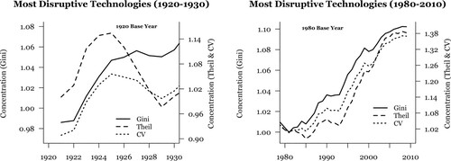
The right panel of Figure 1 displays the analogous evolution of the geography of disruptive innovation for the 1980–2010 period, at the level of commuting zones. Across the different measures of spatial inequality, each series rises quite consistently over the 30-year period. Over this recent period in which new, key technologies are believed to be most profoundly disrupting economic activity in the United States, they are emerging in an increasingly selective regional geography.

One might reasonably wonder whether such geographical patterns are, as we suggest, cyclical. A competing possibility is that the growing geographical clustering of disruptive innovations merely reflects more fundamental shifts in patterns of settlement and overall economic activity. On that logic, since 1980 at least, the United States has been experiencing growing concentration of population and output in larger urban centres (Balland et al., 2020; Black & Henderson, 2003). In reality, these processes are likely to be endogenously related to one another, with innovation as both outcome and driver of agglomeration (Asheim et al., 2011; Duranton & Puga, 2001; Gordon & McCann, 2005). Consideration of these relationships during the Second Industrial Revolution is illuminating. Over the late 19th and early 20th centuries, the US urban system had not yet fully completed its frontier transition (Leyk et al., 2020). The settler population was actively expanding and spreading toward the West and South, widening markets as well as the range of feasible locations for many traded goods to be produced (Kim, 1995). In this light, the patterns in Figure 1 indicating a growing concentration of disruptive innovations are all the more striking. Technological concentration in one period marked by dispersal in population, employment and output hints at the existence of a distinctive and powerful logic shaping the geography of these innovations.

In Figure 2 we seek to further contextualize these findings, revisiting the geography of innovation shown in Figure 1 with some significant differences. First, Figure 2 describes changes in the location of innovation across the entire 90-year study period – a shift that necessitates consistent spatial units (in this case, commuting zones). Second, while the left panel visualizes changes in the geography of the most disruptive innovations, for contrast the right panel shows the spatial evolution of the least disruptive new technologies.

Figure 2. Tracing the geographical concentration of more and less disruptive innovation in the United States, 1920–2010.

Note: Geographical units are commuting zones. See section 3.2 in the text for a detailed discussion of geographical definitions.Source: Authors' elaboration based on HistPat & Lai Database.

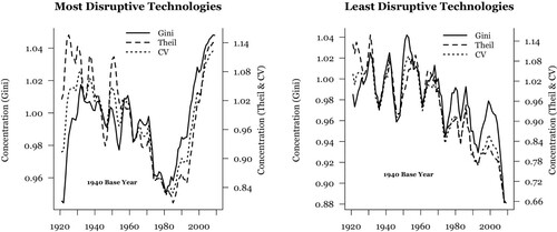
Comparing across the two panels, Figure 2 shows that the most and least disruptive innovations exhibit strongly differentiated locational patterns. The leftmost panel captures the rising spatial concentration of disruptive innovations over the 1920s, with some of the instability seen at the county scale in the Theil series, but also the broadly rising pattern of concentration; this is followed by a gradual spreading out of disruptive innovations from the mid-1930s to approximately 1980, after which we observe once again the spatial concentration during the Third Industrial Revolution. We interpret this to mean that innovations with greater disruptive potential follow a wave-like pattern of rising and then falling spatial concentration that mirrors temporal patterns that economic historians highlight as peaks and troughs of industrial revolutions.

Examining the right panel of Figure 2, we observe that technologies that have the least potential for disruption appear to be spreading out over space over the entire 90-year period. This hints at a deepened diffusion process for the creation of new ideas whose underlying concepts and knowledge bases are more peripheral to the overall technological frontier. As we have seen that some of the least disruptive innovations involve ‘mature’ technologies, it suggests these became more easily accessible, perhaps driven by the wider settlement process underway in the United States. Nonetheless, it is striking that the progressive dispersal of such innovation in an ever-widening circle of locations proceeds even during periods of peak technological upheaval, and even when indicators of population and output grow increasingly concentrated.

4.2. Waves of concentrated disruptive innovation reshape the ranks of regional technological leadership

In this section we explore which cities have become sites of concentrated disruptive innovation. We also consider whether holding a leadership position in disruptive innovation in one period leads to being a leader in a subsequent one.

In a five-year window within each industrial revolution, Table 3 lists the top 25 regions based on counts of disruptive innovation per 1000 inhabitants. It lists counties that are hubs of disruptive innovation in 1925–30, while for the later period it lists commuting zones. Over the 1925–30 period, leading disruptive technology regions were mostly concentrated in the Northeast and Midwest – the old industrial heartland of the electrical–mechanical age. The distribution of disruptive innovations per 1000 across these centres is relatively even, such that those in the middle of the list generate about a third of the number of disruptive innovations per capita as those at the very top. At the very top of the list is Schenectady, home of General Electric, as well as the American Locomotive Company, the latter focused on steam and diesel locomotives, as well as steel production. Larger counties on the list, such as Lucas, Hamilton, New York, Allegheny and Cook, each represent significant industrial cities of the Second Industrial Revolution: respectively, Toledo, Cincinnati, New York, Pittsburgh and Chicago. Though we show measures scaled to population in Table 3, absolute counts of disruptive innovation over this period favour large locations, including many of the biggest urban counties such as Wayne (Detroit), Los Angeles, Cuyahoga (Cleveland), Philadelphia, Milwaukee, St. Louis and San Francisco.

Table 3. Top 25 most disruptive places in each period, according to the number of disruptive patents per 1000 inhabitants.

1925–30			2005–10
County	Disruptive patents (thousands)	Population	Largest city in commuting zone	Disruptive patents (thousands)	Population
Schenectady, NY	$3.111$	$125,021$	San Jose, CA	$14.453$	$2,521,876$
Branch, IN	$2.463$	$23,950$	Boise City, ID	$8.863$	$645,142$
Sullivan, NH	$2.347$	$24,286$	Burlington, VT	$6.951$	$334,495$
Lucas, OH	$1.585$	$347,709$	Fort Collins, CO	$4.998$	$582,859$
Coos, NH	$1.489$	$38,959$	San Francisco, CA	$4.783$	$4,896,022$
Warren, OH	$1.463$	$27,348$	Rochester, MN	$4.649$	$253,379$
New York, NY	$1.458$	$1,867,312$	Poughkeepsie, NY	$4.238$	$931,061$
Hamilton, OH	$1.435$	$589,356$	Austin, TX	$3.952$	$1,779,457$
Rock, WI	$1.267$	$74,306$	Lawton, OK	$3.299$	$183,112$
Essex, MA	$1.179$	$498,040$	Portland, OR	$2.803$	$2,133,238$
Knox, OH	$1.125$	$39,338$	San Diego, CA	$2.679$	$3,104,346$
Essex, NJ	$1.103$	$833,513$	Elmira, NY	$2.599$	$350,074$
Brule, SD	$1.079$	$7416$	Boston, MA	$2.561$	$5,163,543$
Washington, CO	$1.043$	9591	Raleigh, NC	$2.508$	$1,876,821$
Allegheny, PA	$1.038$	$1,374,410$	Palm Bay, FL	$2.424$	$682,251$
Union, NJ	$1.032$	$305,209$	Minneapolis, MN	$2.303$	$3,197,939$
Fairfield, CT	$0.996$	$386,702$	Albany, NY	$2.231$	$1,112,237$
Cook, IL	$0.967$	$3,982,123$	Seattle, WA	$2.181$	$4,285,519$
Hartford, CT	$0.962$	$421,097$	Eugene, OR	$2.122$	$1,045,295$
Bossier, LA	$0.951$	$28,388$	Buffalo, NY	$2.095$	$2,353,374$
Fairfax, VA	$0.950$	$25,264$	Binghamton, NY	$2.014$	$294,870$
Hampton, VA	$0.940$	6382	Manchester, NH	$1.982$	$1,271,163$
Erie, OH	$0.902$	$42,133$	Brick Township CDP, NJ	$1.909$	$1,208,464$
Westchester, NY	$0.898$	$520,947$	Pullman, WA	$1.901$	$82,075$
Richland, OH	$0.895$	$65,902$	Cedar Rapids, IA	$1.878$	$274,746$

The list describing the 2005–10 period looks different in a number of ways. It is more consistently made up of large population centres, which are also drawn from a wider range of regions of the United States. Almost a quarter lie on the Pacific coast, and Sunbelt cities such as Austin and Raleigh bring in the Old South. Regional economies known for leadership in high-technology sectors of the Third Industrial Revolution appear on the list, including San Francisco, San Jose, Austin, Boston and Seattle. Among the smaller places, Rochester, Minnesota and Poughkeepsie, New York, both host large IBM research and design facilities. One difference between the two periods is the degree of concentration of disruptive patents in the more recent period, with San Jose having generated approximately 1.6 times as many disruptive patents as the second-placed location, and almost seven times as many as the middle of the list. By contrast, over the 1925–30 period, the leading county had 1.2 times as many as the second-placed location, and fewer than three times as many as the middle of the list.

Based on this picture, we can ask whether the same regional economies are hubs of innovation across the two study periods. To respond to this question, we again require consistent units. Hence, in Table 4 we aggregate up to the level of 1990 vintage commuting zones. Only four regions that out of the top 25 most disruptive locations in 1925–30 remain so in 2005–10. The overwhelming majority of leading places are leaders in only one period. A similar picture emerges if we measure total patents, such that only half the locations that are in the top 25 in the 1920s remain so in the 2000s. This greater intertemporal consistency no doubt emerges as a consequence of the fact that big populations exhibit greater long-run persistence.

Table 4. Turbulence in the leadership ranks of commuting zones across the 1925–10 period.

			2005–10
			Not in top 25	Top 25
Disruptive patents/capita	1925–30	Not in top 25	$527$	$21$
		Top 25	$19$	$4$
Total disruptive patents	1925–30	Not in top 25	$534$	$12$
		Top 25	$12$	$13$

Note: Because of the need for consistent units in this analysis, we aggregate counties over the 1925–30 period up to the level of commuting zones.

Being at the top in per capita terms means being a centre of the disruptive technologies of the specific industrial revolution at hand. There is substantial turbulence or difference in regional leadership of disruptive technological change from one revolution to another. On a total patenting basis, however, there is less volatility over time, perhaps reflecting some long-term advantage of being a large city-region in the urban system in successfully transitioning as a technology centre from one period to another. Still, almost half of the leaders in the 2000s were not to be found there during the Second Industrial Revolution, reflecting the entrance of major new innovation centres as new technologies rely less on the innovators and inputs from previous rounds, creating what has been termed a ‘window of locational opportunity’ (Scott & Storper, 1987; Storper & Walker, 1989). Long-run stability is most evident among the non-innovative laggards.

4.3. Spatially concentrated disruptive innovation is associated with greater spatial economic inequalities

Next we turn to regression estimates measuring the association between disruptive innovation and either output or income. Table 5 reports estimates for variants of equation (1)(1) $y_{c,t}=d_{c,t}+l{d}_{c,t}+X_{c,t}^{{}^{\mathrm{\prime }}}+u_{c,t}$(1) , which relates changes in location-specific measures of disruptive innovation to changes in local per capita output. In both industrial revolutions, we detect a robust, positive relationship between the marginal instance of local disruptive innovation and economic performance. Models 1 and 2 are differenced between 1920 and 1930, such that the dependent variable is the change in log manufacturing output per worker. In model 1, innovative output, as represented by total patents, is positively and significantly linked to growth in per capita output in manufacturing. Controls behave approximately as expected, including a lagged dependent variable that is negatively and significantly linked to output, indicating a conditional convergence dynamics that fit with state-level evidence on income spanning this period (Barro, 1991). Model 2 disaggregates total patents, with key predictors capturing additional patents granted in the most and least disruptive technology classes over the study period. Disruptive patents remain positively and significantly associated with growth in output per worker. Meanwhile, the addition of least disruptive patents is not significantly related to changes in manufacturing output over this period.

Table 5. Local disruptive innovation and development indicators for the Second and Third Industrial Revolutions, 1920–1930 and 1980–2010.

	Second Industrial Revolution		Third Industrial Revolution
	Differenced $\Delta y_c$		Decadal FE panel
	(1)	(2)	(3)	(4)
All patents (log)	0.085***		0.011*
	(0.018)		(0.005)
Most disruptive patents (log)		0.054***		0.011**
		(0.020)		(0.0043)
Least disruptive patents (log)		0.036		0.0059
		(0.02)		(0.0034)
Population (log)	0.074*	0.094*	−0.072	−0.102
	(0.037)	(0.042)	(0.024)	(0.027)
Urban population share	0.00003	−0.00001
	(0.0001)	(0.0001)
Foreign-born share	−0.0001	−0.0002
	(0.0005)	(0.0005)
Primary inputs	0.914***	0.922***
	(0.172)	(0.174)
Land grant university	−0.052	−0.045
	(0.062)	(0.064)
Post offices	−0.004**	−0.005**
	(0.002)	(0.002)
$y_{c,t-1}$	−0.204***	−0.199***	−0.049	−0.041
	(0.028)	(0.029)	(0.023)	(0.026)
4+ Years College share			0.146	0.078
			(0.108)	(0.116)
Computer employment share			0.279	0.308
			(0.339)	(0.339)
FIRE employment share			2.66***	2.853***
			(0.371)	(0.461)
Manufacturing employment share			0.397***	0.447***
			(0.073)	(0.086)
Period	1920–30	1920–30	1980–2010	1980–2010
State FEs	Yes	Yes	No	No
CZ FEs	No	No	Yes	Yes
Year FEs	No	No	Yes	Yes
Observations	2438	2438	2900	2900
$R^2$	0.148	0.146	0.934	0.904

Note: *$p<0.05$, **$p<0.01$, ***$p<0.001$. Panel models report cluster-robust (CZ-level) standard errors in parentheses. The 1920–30 period reports cluster-robust (state-level) standard errors in parentheses. Unit of observation in models 1 and 2 is the county; and in models 3 and 4 it is the commuting zone. The dependent variable in models 1 and 2 is change in log manufacturing output per worker; the dependent variable in models 3 and 4 is log per capita personal income (PCPI). PCPI is inflation-adjusted to constant 2010 US$.

Based on a decadal panel specification with two-way fixed effects, results for the more recent period up to 2010 track the relationship between changes in disruptive innovation and log PCPI. The inclusion of local fixed effects should absorb bias that arises from differences in overall innovative capacity, as long as this characteristic is relatively stationary; it also accounts for other unmeasured but relatively non-dynamic features of locations. As in model 1 for the 1920s, model 3 confirms that, over this more recent period, increases in local patenting are linked to rising output per head, significant against a threshold of 0.05. Mirroring the estimates for the Second Industrial Revolution shown in model 2, in model 4 we decompose total patents into their extremes: patents in the most disruptive classes, and those in classes deemed to be least likely to be disruptive. The coefficient on disruptive patents is positive and statistically significant at a 0.01% level, the greater precision in the estimate as compared to all patents in model 3 indicating the greater clarity offered by a focus on disruptive innovation. In keeping with model 2, the addition of new, least-disruptive patents is unrelated to changes in PCPI. Meanwhile, the $\text{β}$-convergence process detected in the early period is no longer in evidence.¹⁸

Overall then, for each of the key periods in two industrial revolutions, the regressions in Table 5 suggest that the relationship between overall local patenting and local output or income is partly a function of those innovations that are most disruptive. Considering these relationships in light of the distinctive patterns of geographical concentration of disruptive innovations we document in Figure 1 suggests that disruptive innovation acted as a force spurring growing regional inequalities, whether in terms of manufacturing output per capita in the 1920s, or PCPIs as the Third Industrial Revolution unfolded.

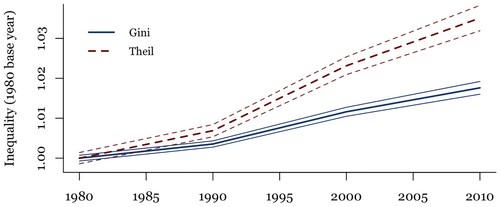
Exploring this idea further, Figure 3 visualizes changes in spatial inequality that emerge from predicted values of local PCPI that emerge from model 4, Table 5, setting all independent variables to 1980 mean levels, except for disruptive innovation, which we allow to change according to actual values. These predictions are then used to build standard inequality indices used above. This figure is not meant to be interpreted as a direct gauge of disruptive innovation's marginal effects; rather, it represents a counterfactual scenario that more directly highlights the how the growing concentration of disruptive innovations in space yields tangible increases in spatial inequality.

Figure 3. A counterfactual scenario relating disruptive innovation and spatial inequality, 1980–2010.

Note: The graph shows changes in per capita personal income (PCPI) inequality, based on model 4 in Table 5, with all predictors except the most disruptive innovations set to 1980 means.

5. CONCLUSIONS: THE FUTURE OF DISRUPTION AND ITS GEOGRAPHIES

Over the past century, disruptive innovations in the United States follow alternating wave-like patterns of rising and falling spatial concentration that closely mimic peak and trough periods of industrial revolutions (David, 1990; Field, 2003). The least disruptive innovations, by contrast, were quite consistently spreading out over the regional geography of the country. Further, there was only partial overlap in the geography of disruptive innovations across the two Industrial Revolutions, with turbulence in the ranks of the most innovative places and thus limited path dependence in disruptive innovation. In contrast, there was mostly stability in the geography of places excluded from the business of leading in the generation of the most disruptive innovations. Finally, we found a robust association between regional disruptive innovation and measures of economic performance. This relationship remains after accounting for the influence of a host of other factors shaping such outcomes, including other markers of innovative effort. Taken together, these results are consistent with the idea that disruptive innovation has played an important role in shaping patterns of spatial economic inequality over the past century.

Still, much more work is required to understand the links between technology and the geography of inequality. It would be particularly interesting to understand more precisely the nature and geography of technology during the peak spatial and interpersonal convergence period of the American economy from 1940 to 1960. What we do not know from this analysis is the precise extent to which the technological contribution to the 1940–80 Great Levelling in both regional development and income inequality was due to the spatial deconcentration of disruptive innovations; to an overall decline in disruptiveness; to a decline in the skill bias of disruptive innovations; or to some as yet unobserved quality of disruptiveness that may have changed between the two high inequality and concentration periods and the intervening Great Levelling. These questions are therefore urgent for further research that would build upon the present results.

Building such an understanding is particularly urgent as we appear to be on brink of a Fourth Industrial Revolution, perhaps based upon breakthroughs in robotics, artificial intelligence, genomics and decarbonization technologies. Historical research, such as we report on in this paper, does not promise the prediction of future processes, but provides a useful framework of questions to ask as such processes begin to unfold. In particular, as these technologies emerge from their current experimental phase, we should carefully consider whether they manifest analogous forms of geographical concentration to their forebears, reinforcing ‘superstar’ agglomerations of knowledge workers, major firms and supply chains, and incomes, but also possibly generating some new superstars in the urban–regional system (Kemeny & Storper, 2020a). In this case, then the contemporary geography of regional economic divergence may be a prelude to another round of uneven development within innovative countries. At the global scale, the current period is different from the Great Divergence of the First Industrial Revolution, as East Asia has now arisen as a third great pole of innovation and world economic growth, and – at least among the three poles of North America, Western Europe and East Asia – per capita incomes are converging. And yet within that third great pole of the world economy, the subnational geography of innovation is highly concentrated. On the other hand, if the upcoming waves of technological disruption are more similar to the disruptions of the Great Levelling, the future of interpersonal and spatial development indicators might look more egalitarian. The social, economic, political and cultural consequences of more versus less egalitarian technological disruption processes are profound; hence, it behoves us to continue deepening the historical understanding of why some disruptions are more spatially concentrated and inegalitarian than others, and to be highly attentive to how the now unfolding new waves of innovation fit in this picture.

DISCLOSURE STATEMENT

No potential conflict of interest was reported by the authors.

Notes

1 While some eschew the term ‘revolution’, preferring instead an image of gradual unfolding, it is widely agreed that a major phase change occurred with early industrialization (Crafts, 2004).

2 The term ‘disruptive’ is itself highly polysemic, used by varied strands of academic work, as well as by journalists, pundits and tech entrepreneurs, through which it has entered the general lexicon. In academic work, the literature in business studies explores the positions of firms whose practices or products disrupt existing industries and markets (e.g., Bower & Christensen, 1995; Christensen et al., 2018). In economics, it is used mostly to characterize major effects on the economy as a whole, wrought through changes in employment, industry structure, productivity, incomes, wages, overall growth and geography (i.e., Bloom et al., 2021). As our review makes clear, the research reported in this paper is situated within this latter tradition.

3 For instance, Lindert and Williamson (2016) date the start of the second industrial revolution at c.1870 and the end c.1920, whereas Jovanovic and Rousseau (2005) argue it spanned the period 1889–1929.

4 Field (2003) has a different, but partially overlapping, formulation, one that puts greater emphasis on the 1929–41 period.

5 While it is worth noting the lively debate around the measurement of the productivity effects of the digital revolution (i.e., Brynjolfsson & Hitt, 1996; Gordon, 2000), there remains little dispute about the broad timing with which information technologies began to restructure the US economy.

6 For all patent documents granted since 1920, see https://bulkdata.uspto.gov/.

7 See http://www.uspto.gov/learning-and-resources/electronic-bulk-data-products/.

8 Each class appearance counts as 1 – there are no fractional counts. However, as explored by Petralia (2020b), an alternate strategy that uses fractional counts produces material similar results.

9 See Hall et al. (2001) for details. For the concordance, see http://www.nber.org/patents/.

10 Our implementation is identical to that described by Petralia (2020b). See Appendix B in the supplemental data online for a detailed explanation of the procedure.

11 For the latest version of this HistPat, see https://dataverse.harvard.edu/dataverse/HistPat/. Petralia et al. (2016) contains a detailed documentation of the methodology used to create it, and a set of tests to discard the existence of potential biases using manually collected data.

12 For the data, see https://www.patentsview.org/download/.

13 We assign patents to locations without taking into consideration the share of inventors per location. For instance, if a patent contains three inventors from Boston and one from Los Angeles, we assign 1 count to each location. We do this for two reasons. This procedure help us to net out the effect of inventive activity becoming more collaborative over time. Using this procedure prevents more populous locations from receiving a disproportionate amount of patent counts. Additionally, disregarding fractional counts makes the comparison between HistPat and more recent data possible. This is because the HistPat database identifies locations in patents but not the inventors, making it impossible to weight contributions.

14 These limitations mean that we cannot simply run one model that spans the entire 90-year study period.

15 For ICPSR 2896, see https://www.icpsr.umich.edu/icpsrweb/.

16 At a detailed subnational scale, information on per capita GDP are only available after 2000.

17 For the original records, see https://catalog.hathitrust.org/Record/002137107/.

18 Concerned with the possibility that our inclusion of a lagged dependent variable might render our estimated standard errors inconsistent, the Appendix in the supplemental data online reports a version of model 4 using the Arellano–Bond estimator. The results remain materially consistent with those presented in the main table.

REFERENCES

- Abramitzky, R., & Boustan, L. (2017). Immigration in American economic history. Journal of Economic Literature, 55(4), 1311–1345. https://doi.org/https://doi.org/10.1257/jel.20151189
- Abramovitz, M. (1986). Catching up, forging ahead, and falling behind. The Journal of Economic History, 46(2), 385–406. https://doi.org/https://doi.org/10.1017/S0022050700046209
- Acemoglu, D. (2002). Directed technical change. Review of Economic Studies, 69(4), 781–809. https://doi.org/https://doi.org/10.1111/1467-937X.00226
- Acemoglu, D., Moscona, J., & Robinson, J. A. (2016). State capacity and American technology: Evidence from the nineteenth century. American Economic Review, 106(5), 61–67. https://doi.org/https://doi.org/10.1257/aer.p20161071
- Acemoglu, D., & Restrepo, P. (2021). Tasks, automation, and the rise in US wage inequality (Working Paper No. 28920). National Bureau of Economic Research (NBER).
- Aghion, P., Akcigit, U., Bergeaud, A., Blundell, R., & Hémous, D. (2019). Innovation and top income inequality. The Review of Economic Studies, 86(1), 1–45. https://doi.org/https://doi.org/10.1093/restud/rdy027
- Aghion, P., & Howitt, P. (2000). On the macroeconomic effects of major technological change. In The economics and econometrics of innovation (pp. 31–53). Springer.
- Akcigit, U., Grigsby, J., & Nicholas, T. (2017). The rise of American ingenuity: Innovation and inventors of the golden age (Technical Report). National Bureau of Economic Research (NBER).
- Allen, R. C. (2009). The British Industrial Revolution in global perspective. Cambridge University Press.
- Allen, T., & Arkolakis, C. (2014). Trade and the topography of the spatial economy. The Quarterly Journal of Economics, 129(3), 1085–1140. https://doi.org/https://doi.org/10.1093/qje/qju016
- Asheim, B. T., Smith, H. L., & Oughton, C. (2011). Regional innovation systems: Theory, empirics and policy. Regional Studies, 45(7), 875–891. https://doi.org/https://doi.org/10.1080/00343404.2011.596701
- Atack, J., & Bateman, F. (1999). Nineteenth-century US industrial development through the eyes of the census of manufactures a new resource for historical research. Historical Methods: A Journal of Quantitative and Interdisciplinary History, 32(4), 177–188. https://doi.org/https://doi.org/10.1080/01615449909598939
- Autor, D. (2019). Work of the past, work of the future (Working Paper No. 25588). National Bureau of Economic Research (NBER).
- Autor, D. H., Katz, L. F., & Kearney, M. S. (2008). Trends in US wage inequality: Revising the revisionists. Review of Economics and Statistics, 90(2), 300–323. https://doi.org/https://doi.org/10.1162/rest.90.2.300
- Autor, D. H., Levy, F., & Murnane, R. J. (2003). The skill content of recent technological change: An empirical exploration. The Quarterly Journal of Economics, 118(4), 1279–1333. https://doi.org/https://doi.org/10.1162/003355303322552801
- Balland, P.-A., Jara-Figueroa, C., Petralia, S. G., Steijn, M. P., Rigby, D. L., & Hidalgo, C. A. (2020). Complex economic activities concentrate in large cities. Nature Human Behaviour, 4(3), 248–254. https://doi.org/https://doi.org/10.1038/s41562-019-0803-3
- Balland, P.-A., & Rigby, D. (2017). The geography of complex knowledge. Economic Geography, 93(1), 1–23. https://doi.org/https://doi.org/10.1080/00130095.2016.1205947
- Barro, R. J. (1991). Economic growth in a cross section of countries. The Quarterly Journal of Economics, 106(2), 407–443. https://doi.org/https://doi.org/10.2307/2937943
- Barro, R. J., & Sala-i-Martin, X. (1991). Convergence across states and regions. Brookings Papers on Economic Activity, 107–182. https://doi.org/https://doi.org/10.2307/2534639
- Baum-Snow, N. (2007). Did highways cause suburbanization? The Quarterly Journal of Economics, 122(2), 775–805. https://doi.org/https://doi.org/10.1162/qjec.122.2.775
- Berger, T., & Frey, C. B. (2016). Did the computer revolution shift the fortunes of US cities? Technology shocks and the geography of new jobs. Regional Science and Urban Economics, 57, 38–45. https://doi.org/https://doi.org/10.1016/j.regsciurbeco.2015.11.003
- Berkes, E., & Gaetani, R. (2021). The geography of unconventional innovation. The Economic Journal, 131(636), 1466–1514. https://doi.org/https://doi.org/10.1093/ej/ueaa111
- Black, D., & Henderson, V. (2003). Urban evolution in the USA. Journal of Economic Geography, 3(4), 343–372. https://doi.org/https://doi.org/10.1093/jeg/lbg017
- Bloom, N., Hassan, T. A., Kalyani, A., Lerner, J., & Tahoun, A. (2021). The diffusion of disruptive technologies (Working Paper No. 28999). National Bureau of Economic Research (NBER).
- Boschma, R., & Van der Knaap, G. (1999). New high-tech industries and windows of locational opportunity: The role of labour markets and knowledge institutions during the industrial era. Geografiska Annaler: Series B, Human Geography, 81(2), 73–89. https://doi.org/https://doi.org/10.1111/j.0435-3684.1999.00050.x
- Bower, J. L., & Christensen, C. M. (1995). Disruptive technologies: Catching the wave. Harvard Business Review, 43(January–February), 43–53.
- Bresnahan, T. F., Brynjolfsson, E., & Hitt, L. M. (2002). Information technology, workplace organization, and the demand for skilled labor: Firm-level evidence. The Quarterly Journal of Economics, 117(1), 339–376. https://doi.org/https://doi.org/10.1162/003355302753399526
- Bresnahan, T. F., & Trajtenberg, M. (1995). General purpose technologies: Engines of growth? Journal of Econometrics, 65(1), 83–108. https://doi.org/https://doi.org/10.1016/0304-4076(94)01598-T
- Brynjolfsson, E., & Hitt, L. (1996). Paradox lost? Firm-level evidence on the returns to information systems spending. Management Science, 42(4), 541–558. https://doi.org/https://doi.org/10.1287/mnsc.42.4.541
- Card, D., Rothstein, J., & Yi, M. (2021). Location, location, location (Discussion Paper No. 21-32). US Census Bureau Center for Economic Studies.
- Carlino, G. A., & Mills, L. O. (1993). Are US regional incomes converging?: A time series analysis. Journal of Monetary Economics, 32(2), 335–346. https://doi.org/https://doi.org/10.1016/0304-3932(93)90009-5
- Christensen, C. M., McDonald, R., Altman, E. J., & Palmer, J. E. (2018). Disruptive innovation: An intellectual history and directions for future research. Journal of Management Studies, 55(7), 1043–1078. https://doi.org/https://doi.org/10.1111/joms.12349
- Comin, D., & Hobijn, B. (2010). An exploration of technology diffusion. American Economic Review, 100(5), 2031–2059. https://doi.org/https://doi.org/10.1257/aer.100.5.2031
- Crafts, N. (2004). Steam as a general purpose technology: A growth accounting perspective. The Economic Journal, 114(495), 338–351. https://doi.org/https://doi.org/10.1111/j.1468-0297.2003.00200.x
- Crescenzi, R., Iammarino, S., Ioramashvili, C., Rodríguez-Pose, A., & Storper, M. (2020). The geography of innovation and development: global spread and local hotspots (Discussion Paper No. 4). LSE Department of Geography and Environment.
- David, P. A. (1990). The dynamo and the computer: An historical perspective on the modern productivity paradox. The American Economic Review, 80(2), 355–361.
- David, P. A., & Wright, G. (2005). General purpose technologies and productivity surges: Historical reflections on the future of the ICT revolution. Economic History, 502002. https://doi.org/10.5871/bacad/9780197263471.003.0005
- David, P., & Wright, G. (2003). General purpose technologies and surges in productivity: Historical reflections on the future of the ICT revolution. In P. David, & M. Thomas (Eds.), The Economic future in historical perspective. Oxford University Press.
- Diamond, R. (2016). The determinants and welfare implications of US workers’ diverging location choices by skill: 1980–2000. American Economic Review, 106(3), 479–524. https://doi.org/https://doi.org/10.1257/aer.20131706
- Dorn, D. (2009). Essays on inequality, spatial interaction, and the demand for skills. PhD thesis, University of St. Gallen.
- Drennan, M. P., & Lobo, J. (1999). A simple test for convergence of metropolitan income in the United States. Journal of Urban Economics, 46(3), 350–359. https://doi.org/https://doi.org/10.1006/juec.1998.2126
- Drennan, M. P., Tobier, E., & Lewis, J. (1996). The interruption of income convergence and income growth in large cities in the 1980s. Urban Studies, 33(1), 63–82. https://doi.org/https://doi.org/10.1080/00420989650012121
- Duranton, G., & Puga, D. (2001). Nursery cities: Urban diversity, process innovation, and the life cycle of products. American Economic Review, 91(5), 1454–1477. https://doi.org/https://doi.org/10.1257/aer.91.5.1454
- Duranton, G., & Puga, D. (2004). Micro-foundations of urban agglomeration economies. In Handbook of regional and urban economics, volume 4, pages 2063–2117. Elsevier.
- Esposito, C. (2021). The geography of breakthrough innovation in the United States over the 20th century (Papers in Evolutionary Economic Geography No. 21.26).
- Feldman, M. P., Kogler, D. F., & Rigby, D. L. (2015). Rknowledge: The spatial diffusion and adoption of rDNA methods. Regional Studies, 49(5), 798–817. https://doi.org/https://doi.org/10.1080/00343404.2014.980799
- Feldman, M. P., & Yoon, J. W. (2012). An empirical test for general purpose technology: An examination of the Cohen–Boyer rDNA technology. Industrial and Corporate Change, 21(2), 249–275. https://doi.org/https://doi.org/10.1093/icc/dtr040
- Field, A. J. (2003). The most technologically progressive decade of the century. American Economic Review, 93(4), 1399–1413. https://doi.org/https://doi.org/10.1257/000282803769206377
- Fishback, P., & Cullen, J. A. (2013). Second world war spending and local economic activity in US counties, 1939–58. The Economic History Review, 66(4), 975–992.
- Foster, J. G., & Evans, J. A. (2019). Promiscuous inventions. In Beyond the meme: Development and structure in cultural evolution (pp. 200–236). University of Minnesota Press. http://www.jstor.org/stable/https://doi.org/10.5749/j.ctvnp0krm.8
- Freeman, C., & Louçã, F. (2001). As time goes by: From the industrial revolutions to the information revolution. Oxford University Press.
- Freeman, C., & Soete, L. (1997). The economics of industrial innovation. Psychology Press.
- Galbraith, J. K., & Hale, J. T. (2014). The evolution of economic inequality in the United States, 1969–2012: Evidence from data on inter-industrial earnings and inter-regional incomes. World Economic Review, 3(2014), 1–19.
- Galor, O. (2011). Unified growth theory. Princeton University Press.
- Ganong, P., & Shoag, D. (2017). Why has regional income convergence in the US declined? Journal of Urban Economics, 102, 76–90. https://doi.org/https://doi.org/10.1016/j.jue.2017.07.002
- Gaubert, C., Kline, P., Vergara, D., & Yagan, D. (2021). Trends in US spatial inequality: Concentrating affluence and a democratization of poverty. In AEA Papers and proceedings, volume 111 (pp. 520–525).
- Giannone, E. (2017). Skilled-biased technical change and regional convergence (Working Paper). University of Chicago.
- Glaeser, E. L., & Gottlieb, J. D. (2006). Urban resurgence and the consumer city. Urban Studies, 43(8), 1275–1299. https://doi.org/https://doi.org/10.1080/00420980600775683
- Goldin, C. D., & Katz, L. F. (2009). The race between education and technology. Harvard University Press.
- Gordon, I. R., & McCann, P. (2005). Innovation, agglomeration, and regional development. Journal of Economic Geography, 5(5), 523–543. https://doi.org/https://doi.org/10.1093/jeg/lbh072
- Gordon, R. J. (2000). Does the ‘new economy’ measure up to the great inventions of the past? Journal of Economic Perspectives, 14(4), 49–74. https://doi.org/https://doi.org/10.1257/jep.14.4.49
- Gordon, R. J. (2017). The rise and fall of American growth: The US standard of living since the Civil War. Princeton University Press.
- Griliches, Z. (1957). Hybrid corn: An exploration in the economics of technological change. Econometrica, 25(4), 501–522. https://doi.org/https://doi.org/10.2307/1905380
- Gyourko, J., Mayer, C., & Sinai, T. (2013). Superstar cities. American Economic Journal: Economic Policy, 5(4), 167–199. https://doi.org/https://doi.org/10.1257/pol.5.4.167
- Haines, M. R. (2005). Historical, demographic, economic, and social data: The United States, 1790–2000. Computerized Data sets from the Inter-University Consortium for Political and Social Research. ICPSR 2896.
- Hall, B. H., Jaffe, A. B., & Trajtenberg, M. (2001). The NBER patent citation data file: Lessons, insights and methodological tools (Working Paper No. 8498). National Bureau of Economic Research (NBER).
- Hall, B. H., & Trajtenberg, M. (2006). Uncovering general purpose technologies with patent data. In C. Antonelli, D. Foray, B. H. Hall, & W. E. Steinmueller (Eds.), New frontiers in the economics of innovation and new technology: Essays in honour of Paul A. David. Edward Elgar.
- Helpman, E. (1998). General purpose technologies and economic growth. MIT Press.
- Helpman, E. (2009). The mystery of economic growth. Harvard University Press.
- Helpman, E., & Trajtenberg, M. (1998a). Diffusion of general purpose technologies. In E. Helpman (Ed.), General purpose technologies and economic growth (p. 85). MIT Press.
- Helpman, E., & Trajtenberg, M. (1998b). A time to sow and a time to reap: Growth based on general purpose technologies. In E. Helpman (Ed.), General purpose technologies and economic growth (p. 55). MIT Press.
- Hunt, J., & Gauthier-Loiselle, M. (2010). How much does immigration boost innovation? American Economic Journal: Macroeconomics, 2(2), 31–56. https://doi.org/https://doi.org/10.1257/mac.2.2.31
- Jovanovic, B., & Rousseau, P. L. (2005). General purpose technologies. In Handbook of economic growth, Volume 1 (pp. 1181–1224). Elsevier.
- Keller, W. (2004). International technology diffusion. Journal of Economic Literature, 42(3), 752–782. https://doi.org/https://doi.org/10.1257/0022051042177685
- Kemeny, T. (2010). Does foreign direct investment drive technological upgrading? World Development, 38(11), 1543–1554. https://doi.org/https://doi.org/10.1016/j.worlddev.2010.03.001
- Kemeny, T. (2011). Are international technology gaps growing or shrinking in the age of globalization? Journal of Economic Geography, 11(1), 1–35. https://doi.org/https://doi.org/10.1093/jeg/lbp062
- Kemeny, T., & Storper, M. (2012). The sources of urban development: Wages, housing, and amenity gaps across American cities. Journal of Regional Science, 52(1), 85–108. https://doi.org/https://doi.org/10.1111/j.1467-9787.2011.00754.x
- Kemeny, T., & Storper, M. (2020a). The fall and rise of interregional inequality: Explaining shifts from convergence to divergence. Scienze Regionali, 19(2), 175–198.
- Kemeny, T., & Storper, M. (2020b). Superstar cities and left-behind places: Disruptive innovation, labor demand, and interregional inequality (Working Paper No. 41). LSE International Inequalities Institute.
- Kerr, W. R. (2008). Ethnic scientific communities and international technology diffusion. Review of Economics and Statistics, 90(3), 518–537. https://doi.org/https://doi.org/10.1162/rest.90.3.518
- Kim, S. (1995). Expansion of markets and the geographic distribution of economic activities: The trends in US regional manufacturing structure, 1860–1987. The Quarterly Journal of Economics, 110(4), 881–908. https://doi.org/https://doi.org/10.2307/2946643
- Kim, S. (2005). Industrialization and urbanization: Did the steam engine contribute to the growth of cities in the United States? Explorations in Economic History, 42(4), 586–598. https://doi.org/https://doi.org/10.1016/j.eeh.2005.03.001
- Kim, S. (2007). Immigration, industrial revolution and urban growth in the United States, 1820–1920: Factor endowments, technology and geography (Working Paper No. 12900). National Bureau of Economic Research (NBER).
- Lamoreaux, N. R., Levenstein, M., & Sokoloff, K. L. (2004). Financing invention during the Second Industrial Revolution: Cleveland, Ohio, 1870–1920 (Working Paper No. 10923). National Bureau of Economic Research (NBER)/
- Landes, D. S. (2003). The unbound Prometheus: Technological change and industrial development in Western Europe from 1750 to the present. Cambridge University Press.
- Leyk, S., Uhl, J. H., Connor, D. S., Braswell, A. E., Mietkiewicz, N., Balch, J. K., & Gutmann, M. (2020). Two centuries of settlement and urban development in the United States. Science Advances, 6(23), eaba2937. https://doi.org/https://doi.org/10.1126/sciadv.aba2937
- Lin, J. (2011). Technological adaptation, cities, and new work. Review of Economics and Statistics, 93(2), 554–574. https://doi.org/https://doi.org/10.1162/REST_a_00079
- Lindert, P., & Williamson, J. (2016). Unequal gains: American growth and inequality since 1700. Princeton University Press.
- Lipsey, R. G., Carlaw, K. I., & Bekar, C. T. (2005). Economic transformations: General purpose technologies and long-term economic growth. Oxford University Press.
- Maddison, A. (2007). Contours of the world economy 1–2030 AD: Essays in macro-economic history. Oxford University Press.
- Manduca, R. A. (2019). The contribution of national income inequality to regional economic divergence. Social Forces.
- Mewes, L. (2019). Scaling of atypical knowledge combinations in American metropolitan areas from 1836 to 2010. Economic Geography, 95(4), 341–361. https://doi.org/https://doi.org/10.1080/00130095.2019.1567261
- Michaels, G. (2008). The effect of trade on the demand for skill: Evidence from the interstate highway system. Review of Economics and Statistics, 90(4), 683–701. https://doi.org/https://doi.org/10.1162/rest.90.4.683
- Mokyr, J. (1990). Punctuated equilibria and technological progress. The American Economic Review, 80(2), 350.
- Mokyr, J. (2010). The enlightened economy an economic history of Britain 1700–1850. Yale University Press.
- Molloy, R., Smith, C. L., & Wozniak, A. (2011). Internal migration in the United States. Journal of Economic Perspectives, 25(3), 173–196. https://doi.org/https://doi.org/10.1257/jep.25.3.173
- Mom, G. (2014). The evolution of automotive technology: A handbook. SAE.
- Moretti, E. (2004). Estimating the social return to higher education: Evidence from longitudinal and repeated cross-sectional data. Journal of Econometrics, 121(1–2), 175–212. https://doi.org/https://doi.org/10.1016/j.jeconom.2003.10.015
- Moretti, E. (2012). The new geography of jobs. Houghton Mifflin Harcourt.
- Morris, E. (2007). From horse power to horsepower. Access Magazine, 1(30), 2–10.
- Moser, P., & Nicholas, T. (2004). Was electricity a general purpose technology? American Economic Review, Papers and Proceedings, 94, 388–394.
- Norton, R. D., & Rees, J. (1979). The product cycle and the spatial decentralization of American manufacturing. Regional Studies, 13(2), 141–151. https://doi.org/https://doi.org/10.1080/09595237900185121
- Ottaviano, G. I., & Peri, G. (2012). Rethinking the effect of immigration on wages. Journal of the European Economic Association, 10(1), 152–197. https://doi.org/https://doi.org/10.1111/j.1542-4774.2011.01052.x
- Partridge, M. D. (2010). The duelling models: Neg vs amenity migration in explaining US engines of growth. Papers in Regional Science, 89(3), 513–536. https://doi.org/https://doi.org/10.1111/j.1435-5957.2010.00315.x
- Perez, C. (2010). Technological revolutions and techno-economic paradigms. Cambridge Journal of Economics, 34(1), 185–202. https://doi.org/https://doi.org/10.1093/cje/bep051
- Petralia, S. (2020a). GPTs and growth: Evidence on the technological adoption of electrical and electronic technologies in the 1920s. European Review of Economic History, 25(3), 571–608. https://doi.org/https://doi.org/10.1093/erehj/heaa022
- Petralia, S. (2020b). Mapping general purpose technologies with patent data. Research Policy, 49(7), 104013. https://doi.org/https://doi.org/10.1016/j.respol.2020.104013
- Petralia, S., Balland, P.-A., & Rigby, D. L. (2016). Unveiling the geography of historical patents in the United States from 1836 to 1975. Scientific Data, 30(3): 160074. https://doi.org/10.1038/sdata.2016.74
- Phene, A., Fladmoe-Lindquist, K., & Marsh, L. (2006). Breakthrough innovations in the US biotechnology industry: The effects of technological space and geographic origin. Strategic Management Journal, 27(4), 369–388. https://doi.org/https://doi.org/10.1002/smj.522
- Pomeranz, K. (2001). The great divergence: China, Europe, and the making of the modern world economy. Princeton University Press.
- Pred, A. R. (1975). Diffusion, organizational spatial structure, and city-system development. Economic Geography, 51(3), 252–268. https://doi.org/https://doi.org/10.2307/143120
- Roback, J. (1982). Wages, rents, and the quality of life. Journal of Political Economy, 90(6), 1257–1278. https://doi.org/https://doi.org/10.1086/261120
- Rodriguez-Pose, A., & Von Berlepsch, V. (2014). When migrants rule: The legacy of mass migration on economic development in the United States. Annals of the Association of American Geographers, 104(3), 628–651. https://doi.org/https://doi.org/10.1080/00045608.2014.892381
- Rosenberg, N., & Nathan, R. (1982). Inside the black box: Technology and economics. Cambridge University Press.
- Rosenberg, N., & Trajtenberg, M. (2004). A general-purpose technology at work: The Corliss steam engine in the late-nineteenth-century United States. The Journal of Economic History, 64(01), 61–99. https://doi.org/https://doi.org/10.1017/S0022050704002608
- Rosenberg, N., & Trajtenberg, M. (2010). A general-purpose technology at work: The Corliss steam engine in the late-nineteenth-century United States. In Studies on Science And The innovation process: Selected works of Nathan Rosenberg (pp. 97–135). World Scientific.
- Ruggles, S., Flood, S., Foster, S., Pacas, J., Schouweiler, M., & Sobek, M. (2021). IPUMS USA: Version 11.0 [dataset]. IPUMS.
- Saxenian, A. (1996). Regional advantage: Culture and competition in Silicon Valley and Route 128, with a new preface by the author. Harvard University Press.
- Schumpeter, J. A. (1943). Capitalism, socialism and democracy. Routledge.
- Scott, A. J., & Storper, M. (1987). High technology industry and regional development: A theoretical critique and reconstruction. International Society and Science, 112, 213–232.
- Soskice, D. (2020). The American knowledge economy (Working Paper No. 51). LSE International Inequalities Institute.
- Storper, M. (1997). The regional world: Territorial development in a global economy. Guilford.
- Storper, M., Kemeny, T., Makarem, N., & Osman, T. (2015). The rise and fall of urban economies: Lessons from San Francisco and Los Angeles. Stanford University Press.
- Storper, M., & Walker, R. (1989). The capitalist imperative: Territory, technology and industrial growth. Basil Blackwell.
- Teixeira, A. A., Vieira, P. C., & Abreu, A. P. (2017). Sleeping beauties and their princes in innovation studies. Scientometrics, 110(2), 541–580. https://doi.org/https://doi.org/10.1007/s11192-016-2186-9
- Tolbert, C. M., & Sizer, M. (1996). US commuting zones and labor market areas: A 1990 update (Staff Report). US Department of Agriculture.
- US Department of Transportation. (2021). Highway statistics. Federal Highway Administration. http://www.fhwa.dot.gov/policyinformation/statistics.cfm
- Vernon, R. (1966). International investment and international trade in the product cycle. The Quarterly Journal of Economics, 80(2), 190–207. https://doi.org/https://doi.org/10.2307/1880689
- Wright, G. (1990). The origins of American industrial success, 1879–1940. The American Economic Review, 651–668.