Internal migration and house prices in Australia

ABSTRACT

Australia is one of the most mobile countries in the world due to internal migration. This study provides the first evidence of the causal impact of internal migration inflow on house price changes across 237 statistical regions in Australia from 2014 to 2019. Employing a spatial correlation approach, the paper indicates that internal migration that amounts to 1% of the initial local area population is associated with a 0.52–0.71% increase in house prices in the three most populated states of Australia. Migration inflow has a significant positive effect on house price changes in metropolitan areas of Sydney and Melbourne rather than non-metropolitan regions.

KEYWORDS:

• internal migration
• housing prices
• Australia
• instrumental variables

JEL:

• R12
• R23
• R31

1. INTRODUCTION

Internal migration is a crucial component of population change and has been widely studied by policymakers and researchers in the regional studies literature. Australia has the highest level of residential mobility through internal migration,¹ which is still increasing at a modest rate, unlike in other developed countries in Europe and the United States (Charles-Edwards et al., 2018). Australian Bureau of Statistics (ABS) data show that internal migration has been a strong contributor to resident population growth in Australia over the past decades. Considerable research effort has been devoted toward understanding the impact of immigration on house prices in Australia (e.g., Moallemi et al., 2021; Moallemi & Melser, 2020), the United States (Saiz, 2007; Saiz & Wachter, 2011), the UK (Sá, 2015), Canada (Akbari & Aydede, 2012), Switzerland (Degen & Fischer, 2017) Spain (Gonzalez & Ortega, 2013) and New Zealand (Coleman & Landon-Lane, 2007; Stillman & Maré, 2008). However, only a few studies have examined the relationship between internal migration and house price changes (e.g., Howard & Liebersohn, 2021; Stillman & Maré, 2008; Tyrcha, 2020; Wang et al., 2017). To our knowledge, no study has been conducted to investigate the causal impact of internal migration on house prices in Australia.

This paper studies the relationship between internal migration and house price changes in Australia’s three most populated states – New South Wales, Victoria and Queensland – which together accounted for 78% of a 25.4 million total population and had 83% of the total value of residential dwellings in June 2019.² According to ABS data, the total resident population in New South Wales, Victoria and Queensland increased by 9.1%, from 18.1 million in 2014 to 19.8 million in 2019. In the same period, internal migration made up to 17.9% of population growth. Population growth through overseas migration might not be a significant driver for housing price growth in Australia as immigrants rarely buy a property and a vast majority rent for several years (Dowling, 2019). Population growth through births adds no housing supply to the market, and while deaths may add some supply, it is not a significant number. Therefore, we hypothesized that examining where Australian residents choose to relocate and settle is a better indicator of where housing price growth is to be expected. Using ABS data by region, we studied annual house price changes in the 2014–19 period across 237 statistical areas level 3 (SA3), which are geographical areas that generally have a population of between 30,000 and 130,000 people and are designed to provide a regional breakdown of Australia. The panel data cover the six years since house price data for small areas or across SA3 regions are available from 2014.

Our data allow us to measure annual house price changes and the spatial concentration of migrants at SA3-level disaggregated statistical areas, rather than state-, metropolitan- or city-level data, which is crucial for studying the local economic impact of internal migration. Internal migration is the primary channel through which the population adjusts to regional labour and housing market conditions (Greenwood & Hunt, 1984; Vermeulen & Van Ommeren, 2009); therefore, we estimate the impact of migration inflow rate rather than population growth on house price changes with appropriate local area controls. A spatial correlation approach is employed in which the annual change in house prices in different geographical areas is regressed on the annual inflow of migrants in that same area along with appropriate controls. The endogeneity problem arises due to the simultaneous causality between migration flows and house price changes. On the one hand, low house prices may attract migration, so that one would expect a negative correlation between the two variables; and, on the other, migration should increase house prices, so that a positive correlation between the two variables is expected. Our paper provides evidence of the causal relationship between internal migration and housing prices by employing a manually constructed instrument that matches the shift–share instrument used in the immigration literature. An endogeneity problem may also occur due to omitted variables that help to explain both growths in migration and house prices. Thus, we use lagged values of the local unemployment rate and changes in local wages and the number of jobs to capture omitted variables and establish causality between migration and house prices.

The causal relationship between internal migration and house price growth in Australia is a compelling topic to study for at least three reasons. First, internal migration is three times that of international migration, affecting the lives of far more people, despite its being given much less attention in political debates and planning processes.³ This is mainly due to the limited or outdated data on internal migration flows, particularly at the local level. Hence, new narratives from different countries will increase our knowledge of the population mobility effect on the local housing markets.

Second, the estimated sign and magnitude of internal migration impact on housing prices could vary across different regions within a country, which might provide a piece of valuable knowledge to local governments and/or policymakers. House prices are an essential source of human capital accumulation and play an important role in fuelling the growth or decline of economies (Glaeser & Gyourko, 2005; Miller et al., 2011).⁴ Internal migrants and their positive (negative) influence on local housing markets play a crucial role in fostering (slowing down) local economic development. Although governments have much less control over internal migration compared with international migration, they could develop housing policies, for example, affordable housing supply both for the existing migrants and the potential newcomers – based on the potential impact of migration inflows on their local housing markets.

Third, over the past few years, property experts have strongly argued that internal migration away from Australia’s big cities is causing house prices to increase in non-capital city locations.⁵ Testing the validity of this argument could provide valuable insights for property investors.

The findings of the study show that there is a significant local economic impact of internal migration in Australian cities. Internal migration pushes up the demand for housing in migration-receiving areas and results in house price increases. The two-stage least squares (2SLS) regression analysis results suggest that new migrants that amount to 1% of the initial local area population are associated with point estimates of 0.52–0.71% increase in house prices. When we benchmark our results against the results reported by previous research, we see that housing markets in Australian cities behave similarly to those in China, New Zealand and Sweden with a slightly lower coefficient estimate, that is, the positive impact of internal migration on the housing prices ranges from 0.71% for Chinese cities (Wang et al., 2017) to 0.91% in Swedish cities (Tyrcha, 2020), and up to 0.81–1.31% in New Zealand (Stillman & Maré, 2008). We also investigated if the local house price effect of internal migration differs across metropolitan (the greater capital cities) versus non-metropolitan (the rest of the states) statistical areas. Our results suggest that migration inflow has a significant positive effect on house price changes in metropolitan areas such as Sydney and Melbourne rather than non-metropolitan areas in Australia.

Population growth and decline through migration impact residents and have significant social, economic and policy implications. Each individual relocation decision contributes to the broader migration patterns that will help shape our regions, cities, states and territories in the future. The results obtained for Australia could provide essential insights into the regional economic impact of internal migration for other highly urbanized countries, such as New Zealand, Canada and the United States, with very mobile societies. Our paper contributes to the literature on internal migration and house prices in four ways. First, we analyse the impact of migration on house prices using an explicitly regional approach, covering both metropolitan and non-metropolitan areas, as opposed to previously published articles which examined the causal impact of internal migration on housing rents (Howard & Liebersohn, 2021) and prices (Wang et al., 2017) by focusing only on metropolitan areas in the United States and China, respectively. Second, we add to the limited literature on the causal link between internal migration and house prices. After controlling for economic drivers (disparities in the unemployment rate, number of jobs and wages) and non-resident family/friend ties, we find that migration flows raise house prices. Therefore, we argue that the correct causal link is from internal migration flows to housing prices and the relative housing prices are not the reason for inter- and/or intraregional movements. Third, we account for endogeneity in the migration and housing relationship through a commonly used instrumental variables (IV) model, based on the shift–share instrument used in the immigration literature, and employ Jordà’s (2005) local projections (LP) methodology to have a better understanding of the dynamic impact of migration on house prices. Based on sequential regressions of the endogenous variable shifted forward, it further allows us to estimate impulse response functions directly, without specifying or estimating the unknown true multivariate dynamic process, which in turn leads us to measure the diffusion of migration shock to prices over time. Fourth, to date, there is no comprehensive analysis of the impact of internal migration on housing in Australia, a country with the highest level of residential mobility, or any other countries in Southeast Asia and Oceania, and this paper aims to fill that gap.

The remainder of the paper is structured as follows. Section 2 reviews the existing research on the impact of migration on house price changes in several countries. Section 3 briefly discusses population mobility in Australia. Section 4 introduces the methodology. Section 5 presents the results. Section 6 concludes.

2. LITERATURE REVIEW

Migration and regional development studies are often divided between the analysis of the rationale for migration and the impacts of migrants on the local and regional economies, their role and incorporation in societies. Within the first strand of literature, there are four main approaches to better understand the key determinants of population mobility through international and/or internal migration. Whilst neo-classical economic theory stresses relative earnings (regional wage gaps) and employment prospects (differences in unemployment rates), the regional restructuring approach interprets migrations as being dependent on changing regional capital investments and de-investments (Kemper, 2004). Apart from economic explanations, social network theories have been proposed to explain migration flows based on extended local ties to friends and family (Mulder & Cooke, 2009). Lastly, housing has been accepted as one of the most influential factors not only for intraregional residential moves but also for internal migrations within a country since the spatial variation of housing prices may influence decisions about whether to move or stay in various locations (Kemper, 2004; Palomares-Linares & Van Ham, 2020). To date, a considerable amount of research has been conducted on the importance of housing market conditions such as housing price differentials and housing supply constraints for internal migration dynamics (e.g., Gabriel et al., 1992; Molloy et al., 2011; Zabel, 2012, for the United States; Cameron et al., 2006, for the UK, Burnley et al., 2007, for Australia; Mulhern & Watson, 2009, for Spain; Vermeulen & Van Ommeren, 2009, for the Netherlands; and Cannari et al., 2000, for Italy) and the impact of homeownership on the (im)mobility of behaviour of households (e.g., Helderman et al., 2004; Palomares-Linares & Van Ham, 2020).

The above-mentioned papers, which use housing market dynamics as a determinant of internal migration, mainly employed non-structural models without considering the endogeneity between house prices and migration flows. For instance, Molloy et al. (2011) carried out descriptive data analysis to argue that the housing market contraction explains the recent drop in migration in the United States. Burnley et al. (2007) analysed large sample surveys of movers in explaining which housing factors were involved in welfare migration to and from large Australian cities. Several researchers used logistic regression models to evaluate either the effects of house price differential on interregional population mobility (Cannari et al., 2000; Gabriel et al., 1992) or the effects of homeownership on internal migration patterns (Palomares-Linares & Van Ham, 2020) or the probability of making a residential move (Helderman et al., 2004). Mulhern and Watson (2009) used a spatial error and spatial autoregression models to understand the migration patterns for Spanish provinces and found that internal migration is determined by a combination of economic explanatory variables, including the differentials in wages, unemployment and house prices between provinces. These papers have mainly used lagged explanatory variables to avoid a possible causality problem between house prices and migration. Furthermore, Zabel (2012) studied the role of the housing market (e.g., homeownership rates and relative house prices) in the migration rates using the vector autoregressive (VAR) models and outlined response functions based on labour demand and supply shocks. To our knowledge, Vermeulen and Van Ommeren (2009) is the only study that has explored the effect of housing market dynamics on internal migration, considering the endogeneity between the two. The researchers concluded that net internal migration in the Netherlands was primarily determined by regional housing supply, not employment growth.

The second strand of literature, which investigates the effects of migration on local and regional housing markets, has mainly focused on international migration and indicated that immigration has an ambiguous impact on housing prices. Although Saiz (2007), Stillman and Maré (2008), Degen and Fischer (2017) and Akbari and Aydede (2012) have provided positive impact estimates for the United States, New Zealand, Switzerland and Canada, respectively, several researchers (Accetturo et al., 2014; Hatton & Tani, 2005; Saiz & Wachter, 2011; Sá, 2015) suggested negative impacts of immigration on average house prices mainly when focusing on small local areas, that is, neighbourhoods within metropolitan areas. The displacement of (wealthy) natives from these neighbourhoods is the main argument used to explain these negative findings.

There has been scarce literature published on the impacts of internal migration on the local and regional housing markets. Previous research has primarily focused on the effects of internal migration on regional growth and convergence (e.g., Fratesi & Percoco, 2014; Kubis & Schneider, 2016; Ozgen et al., 2010; Østbye & Westerlund, 2007). Only a handful of papers have investigated the impact of internal migration on urban housing markets and found that high in-migration in certain areas lead to an increase in housing prices and/or rents (Jeanty et al., 2010). For instance, Howard and Liebersohn (2021) examined the effect of internal migration on housing markets through the aggregate rent increase in all US cities and found that changing migration demand explains 54% of the rent increase and 75% of the consumer price index (CPI) rent increase in the United States from 2000 to 2018. Wang et al. (2017) investigated how interregional migration and rural–urban migration affect urban housing prices in Chinese cities and found that a 1% increase in interregional migrants (rural-to-urban migration) resulted in a 0.70% (0.34%) increase in housing prices when controlling for other relevant factors. Stillman and Maré (2008) examined how population change in New Zealand, through international and internal migration flows, has affected rents and sales prices of both apartments and houses from 1996 to 2006. The study used data from five censuses and revealed that increases in net internal migration flows are associated with higher house prices, that is, a 1% increase in the New Zealand-born population is associated with a 0.81–1.31% increase in house prices. Increases in the immigrant population, in contrast, are negatively associated with house price changes as a 1% population increase from immigrants is associated with a 0.48–0.98% decrease in house prices. Finally, Tyrcha (2020) examined the impact of both internal migration and immigration on the housing market across 284 Swedish municipalities from 2000 to 2015 and concluded that house prices in an area increase by 0.91% with an internal migration impact of 1% of the initial population of the same local area. The papers that study the impact of migration on housing prices mainly used the economic structural models, the use of which are limited by the availability of justified instruments. Structural models result in parameters with particular economic content that can help test hypotheses directly related to economic policies. Our paper contributes to this strand of literature by showing that the correct causal link is from internal migration to house price changes.

Finally, existing research on the Australian experience of internal migration has mostly focused on the main characteristics of internal migrants, such as the age, gender, birthplace, labour force and education; the determinants of migration flows (Bell & Cooper, 1995; Bell & Hugo, 2000; Jarvie, 1989; Rowland, 1979); and the relationship between international migration inflow and internal outmigration within the context of global cities (Burnley, 1996; Burnley et al., 2007; Ley, 2007).⁶

3. POPULATION MOBILITY IN AUSTRALIA

Australia is exceptionally urbanized, despite being relatively sparsely populated. Net overseas migration has been the main driver of Australia’s recent population growth, adding up to 64% of the population increase in 2016–17, whereas it represented only 33.4% of Australia’s population growth in 1976–77 (Simon-Davies, 2018). Internal migration, on the other hand, has been reshaping the geographical distribution of population in the country, leading to growth on the fringes of the major cities, as well as coastal centres, with simultaneous loss from parts of remote Australia (Charles-Edwards et al., 2018). According to the ABS, internal migration is the movement of people from one defined area to another within a country, and it is measured by interstate migration and regional internal migration. While the former is the net gain or loss of population through the movement of people from one state or territory of usual residence to another, the latter is the movement of people from one region to another within the country and includes both inter- and intra-state movements. Previous research has shown that Australia is among the most mobile societies in the world with 15% of the population changing their address within the country in the year before the 2016 Census, and 39% changing their address in the five years before the Census. Across the world, on average, 7.9% of people move domestically each year, while 21% move at least once every five years (Bell et al., 2015). Although a long-term decline in internal migration has been observed in a number of developed countries over recent decades, including the United States and Australia (Champion et al., 2017), the 2016 Census saw a moderate increase in Australian internal migration (Charles-Edwards et al., 2018).

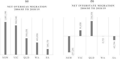
Figure 1 illustrates population mobility during the 2005–19 period in the five most populous states of Australia. In the 15 years before 2019, New South Wales had the largest number of overseas migrant inflow (1,081,190 people), followed by Victoria (968,340) and Queensland (544,430). New South Wales had a strong countervailing population flow of net overseas migration and net interstate migration as the arrival of a large number of overseas immigrants to the state offset departures of the resident population through interstate migration, especially from Sydney (Figure 1). South Australia has also experienced a similar pattern to New South Wales, although on a smaller scale: 189,170 net overseas migrants in, while experiencing a net loss of 62,794 interstate migrants. Queensland, in contrast, had a substantial gain in interstate migration (238,558 people) and received far fewer international immigrants over the same period. Queensland recorded the highest gain in interstate migration, that is, annual average net interstate migration of 17,129 people from 2004 to 2019. Western Australia recorded a net gain of 403,950 overseas immigrants, but the state had a negative number of (−2721) net interstate migration. Hence, the link between overseas migration and interstate migration within Australia’s urban system varies widely across the states. New South Wales and South Australia have experienced offsetting migration flows as net interstate migration losses are seemingly associated with net overseas migration gains. Victoria and Queensland, in contrast, have attracted both overseas and interstate migration.

Figure 1. Net overseas migration (a) and net interstate migration (b) in five main states of Australia.

Source: Australian Bureau of Statistics (ABS) 34120 Migration, Australia.

Apparently, at the state-level aggregate data, net interstate migration is equal to net regional internal migration as intra-state migration flows cancel out each other. In each state, every movement ‘into’ a region is matched by a movement ‘out’ from another region. However, the interstate and regional internal migration certainly differ at the disaggregated SA3 level. This paper uses regional internal migration flows across the SA3 areas to investigate how both inter- and intra-state migration flows affect housing prices in Australia.

4. EMPIRICAL SPECIFICATION

Based on the standard approach in the literature (Saiz, 2007; Sá, 2015), the following model is used to estimate the effect of internal migration on house prices: (1) $\mathrm{\Delta }\ln (H{P}_{i,t})=\beta \left({\displaystyle \frac{Migrant{s}_{i,t-1}}{Populatio{n}_{i,t-2}}}\right)+\alpha X_i+\delta Y_{i,t-1}+\rho \mathrm{\Delta }{Z}_{i,t-1}+{\mathrm{\varnothing }}_i+{\mathrm{\Lambda }}_t+\mathrm{\Delta }{\epsilon }_{i,t}$(1) where $\mathrm{\Delta }\ln (H{P}_{i,t})$ is the change in the log of the median house sales price in each SA3 area $i$ between years $t-1$ and $t$. The main independent variable is the annual inflow of migrants in year $t-1$ divided by the initial population in year $t-2$ in a local area. Given the nature of housing markets, the main specification uses the migration inflow lagged one period with respect to changes in house prices. The coefficient $\beta$ can be interpreted as the percentage change in house prices corresponding to an annual inflow of migrants equal to 1% of the initial local population (Sá, 2015). The independent variable of interest is the normalized migration flow as it is defined as the inflow of migrants into SA3 area $i$ during a particular year divided by the local area’s initial population. As highlighted by Sanchis-Guarner (2017), standardizing migration flows by initial population stock deals with the fact that regions of different sizes have different population and house price dynamics (Wozniak & Murray, 2012), and it eliminates any unobservable factors that might equally affect both the numerator (migration flow) and the denominator (original local population).

In equation (1), $X_i$ stands for initial local area attributes such as having a coastline and total land area. The log of SA3-level land area may capture supply factors related to land availability (Saiz, 2007). $Y_{i,t-1}$ stands for one-year lagged local area characteristics, which may affect house prices, and includes the local unemployment rate to control for local macroeconomic conditions and the housing demand. $\mathrm{\Delta }{Z}_{i,t-1}$ stands for time-varying area characteristics, that is, change in local wages and change in the number of jobs. The variables of the unemployment rate, number of jobs and local wages are well-known essential determinants of housing prices/rents (Jud et al., 1996; Saiz, 2007). Finally, ${\mathrm{\varnothing }}_i$ and ${\mathrm{\Lambda }}_t$ stand for the state-level area fixed effects and time-fixed effects, respectively.

4.1. Instrumental variables (IV)

The dominant methodology used in the empirical literature on migration impacts is the spatial correlation approach in which the change in house prices in different geographical areas is regressed on the inflow of migrants in that same area and appropriate controls (Saiz, 2007). In the absence of a well-identified exogenous shock to migration, for example, ethnic German migrants who were exogenously allocated upon arrival to specific regions by government authorities (Glitz, 2012) or immigration shock after the Mariel boatlift in Miami (Saiz, 2003),⁷ there are four main drawbacks in estimating the causal effect of migration on housing prices.

The first problem arises due to the fact that migration and house prices may be spatially correlated because of common fixed influences such as the climate or local amenities. To address this problem, in line with previous research by Sá (2015), Saiz and Wachter (2011), Saiz (2007) and Coleman and Landon-Lane (2007), our regression model is estimated with the dependent variable in first differences. This eliminates or differences out time-invariant, area-specific factors that affect migration flows and the level of house prices. As a further step, we have included state-level area fixed effects because there might still exist some unobserved factors at the state-level correlated with changes in house prices and changes in migrant stocks. Without considering those, our estimation would be biased (Sá, 2015; Sanchis-Guarner, 2017).

The second problem concerns the length of time that it may take for migration to affect house prices; housing prices cannot adjust immediately. Following Saiz (2007), we estimate the change in house price from $t-1$ to t as a function of one-year lagged migration inflow at $t-1$ divided by total resident population at $t-2$. By using lags of the control variables, we accommodate awareness that house prices do not adjust instantaneously to changes in fundamentals.⁸

The third problem is the endogeneity issue that may occur due to omitted variables that help to explain both growths in migration and house prices. In this paper, we have used lagged values of the local unemployment rate (Saiz, 2007; Sá, 2015) and also lagged changes in local wages (Howard & Liebersohn, 2021; Sanchis-Guarner, 2017) to capture omitted variables and establish causality between migration and house prices. Another source of endogeneity problem arises due to the simultaneous causality between migration flows and house price changes. The direction of causality is not clear because migrants are not randomly allocated across geographical areas, that is, a self-selection endogeneity problem. The sign of bias is difficult to predict ex-ante. On the one hand, migrants may locate in more prosperous areas where house prices are growing faster. On the other, it is reasonable to expect that, controlling for economic conditions, migrants would choose to locate in areas where house prices are growing more slowly (Sá, 2015).

The fourth problem is the measurement error that will lead to attenuation bias, and which is likely to play an important role in migration studies due to the longitudinal nature of the conducted exercise. To net out the district-specific housing effects, we have incorporated state-fixed effects and time-fixed effects that are likely to absorb the permanent factors. Due to the involvement of these effects, our variable of interest (one-year lagged share of migrants) has very little identifying variation left, allowing any sampling error in this variable to play a disproportionately big influence. As a result, even minor sampling errors are amplified, and the remaining variation in the migrant share is outweighed with ease (Aydemir & Borjas, 2011).

To address the simultaneous causality issue and the measurement error problem, we have deployed an instrument for the predicted recent distribution of the migrants based on the past spatial concentrations of migrants – they tend to move to areas where other migrants settled previously (Thomas, 2019). Empirical evidence of internal migration dynamics has hinted at the importance of non-resident family members and/or friends as an attraction factor encouraging and directing migration towards locations where the family/friends live, even as a motive for long-distance (e.g., inter-state) migration in addition to employment and education motives (Burnley et al., 2007; Cooke et al., 2016; Das et al., 2017; Pettersson & Malmberg, 2009; Silverstein & Giarrusso, 2010). Relying on such evidence, an IV based on the settlement pattern of migrants in an earlier period is constructed. More specifically, we have used the settlement pattern of migrants in 2007⁹ to predict the geographical distribution of migrants in the current period. Our identification strategy is based on the tendency of newly arriving migrants to settle in areas where previous migrants from the same area have already settled. We construct and use the following instrument for the inflow of migrants in SA3 region i as a share of the initial local population that matches the shift–share instrument used in the immigration literature: (2) ${\displaystyle \frac{{\sum }_r{\gamma }_{ri0}Migrant{s}_{rt-1}}{Populatio{n}_{it-2}}\mathrm{where}{\gamma }_{ri0}={\displaystyle \frac{migrant{s}_{ri0}}{totalmigrantsmoveou{t}_{r0}}}}$(2) Thus, ${\gamma }_{ri0}$ is the share of migrants who departed from SA3 region r that moved into or settled in SA3 region i in the base year $t_0$. Indeed, ${\gamma }_{ri0}$ gives the direction of migration, namely, flows from and to SA3-level geographical areas and provides a measure of the size of the network from region r in each region i. We nominated 2007 as the base year because regional internal migration estimates data at the SA3 level are available from 2007. $Migrant{s}_{rt-1}$ is the total number of migrants that move out of region r in year t – 1; therefore, the predicted inflow of migrants from region r in year t – 1 that choose to locate in region i is ${\gamma }_{ri0}\times Migrant{s}_{rt-1}$. Summing across all SA3 regions of origin across the country, we obtain a measure of the predicted migration inflow in region i in year t – 1. Our analysis considers 328 SA3 regions of origin across all states and territories of Australia. As the migrants’ country-of-birth information is not available in our dataset (ABS Data by Region at the SA3 level), it is not possible to analyse the separate impact of native versus foreign-born residents’ mobility on house prices.

4.2. Instrumental variables local projections (IV-LP) methodology

To have a better understanding of the dynamics of internal migration and house prices, we further apply LP methodology and obtain impulse response functions (IRFs) from one-step-ahead forecasts. Jordà (2005) shows that IRFs can directly be obtained, without specifying or estimating the unknown true multivariate dynamic process, for instance, through a vector autoregression. The obtained IRFs are robust to misspecification of a data-generating process and can be estimated through a simple univariate framework (Favara & Imbs, 2015). Besides, employing an LP methodology will further allow us to measure the diffusion of migration shock to housing prices accumulated over time, including a set of controls, and can easily accommodate with IV methodology. (3) $\ln (HP{)}_{it+h}-\ln (HP{)}_{it-1}={\beta }^h\left({\displaystyle \frac{Migrant{s}_{i,t-1}}{Populatio{n}_{i,t-2}}}\right)+{\alpha }^h{X}_i+{\delta }^h{Y}_{i,t-1}+{\rho }^h\mathrm{\Delta }{Z}_{i,t-1}+{\varphi }_i^h+{\mathrm{\Lambda }}_i^h+\mathrm{\Delta }{\epsilon }_{i,t+h}$(3) where our dependent variable denotes the response variable of interest, the change in house price in region i from the base year t – 1 up to year t + h with h = 0, 1, … , H, which is estimated by LP regression methods using our shift–share IV as the instrument for $\left({\displaystyle \frac{Migrant{s}_{i,t-1}}{Populatio{n}_{i,t-2}}}\right)$. The coefficients of interest are therefore the IV estimates of ${\beta }^h$ for h = 0, 1, … , H.¹⁰

5. RESULTS

5.1. Data and descriptive analysis

This paper uses two main data sets published by ABS: (1) Migration, Australia (cat. no. 3412.0), which includes estimates of internal migration down to statistical areas, that is, local areas and sub-populations; and (2) Data by region (cat. no. 1410.0), which contains population, economy and industry, income, employment, and total land area data within regions across Australia, from 2013 to 2019. According to the ABS non-census and intercensal statistics, the SA3s are geographical areas that generally have a population of between 30,000 and 130,000 people and are designed to provide a regional breakdown of Australia. In the major cities, SA3s represent the area serviced by a major transport and commercial hub, whereas in regional areas SA3s represent the area serviced by regional cities that have a population of over 20,000 people. In outer regional and remote areas, SA3s represent areas that are widely recognized as having a distinct identity and similar social and economic characteristics. SA3s are classified into two groups: the greater capital city statistical areas (GCCSA) and rest of state statistical areas (RSSA). The former are geographical areas designed to represent the functional extent of each of the eight state and territory capital cities, that is, Greater Sydney, Greater Melbourne, Greater Brisbane, etc., and to reflect labour markets using the 2011 Census travel-to-work data. Within each state and territory, the areas not defined as being part of the greater capital city are represented by rest of state regions such as rest of New South Wales, rest of Victoria and rest of Queensland.

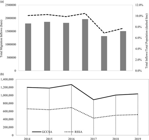
We studied the median house sale price data, provided by the ABS data by region: economy and industry, across 237 SA3 areas in Australia and observe that housing prices increased by 31.9%, on average, in the three states of New South Wales, Victoria and Queensland during the 2014–19 period. Whilst house prices in GCCSAs increased by almost 38%, the average house price increase in RSSAs was only 20.5%. We examined price changes for separate houses only, rather than the attached dwelling types such as semi-detached/terrace houses and apartments/flats because Australia’s cities are all highly suburbanized with low-density urban expansion, for example, almost 76% of the housing stock consists of detached houses, with very little high-density housing except in Sydney (Forster, 2006; Shearer & Burton, 2019). Total migration inflows in the three states are shown in Figure 2(a). The share of migrants in total resident population decreased from 10.3–10.5% in 2014–16 to 7.7–7.8% in 2018–19. The lowest level of internal migration within the three states occurred in 2017 when migration inflows were 6.9% of the total resident population. Studying the decline in internal migration levels in Australia, Kalemba et al. (2020) found that the strong impact of population ageing on the decline in internal migration has been fully counteracted by the positive effects of education and immigration. Furthermore, the behavioural effects are found to be the principal factor explaining this downward trend. Figure 2(b) exhibits total migration inflows in GCCSAs and RSSAs between 2014 and 2019. The annual average migration inflows were 1,095,575 people for the greater capital cities and 572,512 people for the rest of the states.

Figure 2. (a) Total migration inflows in New South Wales, Victoria and Queensland; and (b) total migration inflows in greater capital city statistical areas (GCCSA) and rest of state statistical areas (RSSA).

Source: Calculated by the authors.

Table 1 provides further summary statistics for our dataset. House prices, on average, increased 4.1% per year across our sample during the period under consideration. There is a considerable variation behind this average, that is, the greatest reduction in house prices was recorded in Queensland’s Central Highlands and Outback-South in 2015 and 2016, respectively, where the house prices decreased more than 35%. On the other hand, the most significant increase was registered in 2017 in Loddon-Elmore (Victoria), where house prices increased by more than 25%. Turning to our variable of interest, the SA3-level statistical area received an average annual inflow of 9.1% of its initial population. The largest increases were registered in Queensland’s Brisbane-Inner and Ormeau-Oxford, where, in 2017, the inflow of migrants increases by 18%. In contrast, the lowest increase was in Broken Hill-Far West and Griffith–Murrumbidgee (West) in New South Wales, which recorded a yearly inflow of migration equivalent to 4.1% and 3.6% of their initial population, respectively.

Table 1. Descriptive statistics.

Variables	Mean	SD	Minimum	Maximum
$\mathrm{\Delta }$log Median House Sale Price	0.041	0.079	−0.416	0.257
Migrants at t – 1/Resident Population at t – 2	0.091	0.026	0.037	0.179
Number of Dwellings Approved at t – 1/Population at t – 1	0.008	0.007	0.000	0.073
Unemployment Rate at t – 1	5.683	2.513	1.260	22.900
Δ log Median Wage at t – 1	0.024	0.015	−0.086	0.113
Δ log Number of Jobs at t – 1	0.015	0.031	−0.122	0.176
log Land Area	10.850	2.596	6.971	17.951
Coastal Dummy	0.245	0.431	0.000	1.000

Note: $\mathrm{\Delta }$ represents the first difference.

5.2. Regression analysis

Table 2 presents the results of the two-stage least squares (2SLS) regression analysis of equation (1) using data for 237 SA3 areas. The dependent variable is the change in the log of the median house sale price, and the main variable of interest is migration inflow relative to the total population in the previous year. In all specifications, the standard errors are clustered at the SA3 area level. A suitable strategy to address the endogeneity issue is to use variation in migrant flows that is convincingly exogenous to the evolution of housing prices (Saiz, 2007). As defined in equation (2), we constructed and employed an IV that captures the past spatial concentration of migrants. For the instrument to be valid, it must be correlated with the share of internal migration in the resident population, but uncorrelated with the local shocks that affect house price changes, subject to the controls, fixed area and time effects. In the first stage of the 2SLS regression, the dependent variable is the annual inflow of migrants in year $t-1$ divided by the initial population in year $t-2$ in a local area, whereas the main explanatory variable is the instrument. The estimated value for the first-stage coefficient is between 0.908 and 0.975¹¹ across models of interest and is significant at the 1% level. Such a finding suggests a strong correlation between the current and the predicted geographical distributions of the migrants.

Table 2. Internal migration inflows and house price changes with instrument.

	IV estimation results
Variables	[1]	[2]	[3]	[4]	[5]	[6]	[7]	[8]	[9]
Migrants at t – 1/Resident Population at t – 2	0.429*** [0.022]	0.406*** [0.048]	0.617*** [0.047]	0.712*** [0.071]	0.638*** [0.093]	0.667*** [0.086]	0.628*** [0.087]	0.518*** [0.009]	0.709*** [0.116]
log Land Area			−0.005*** [0.001]	−0.009*** [0.001]	−0.008*** [0.001]	−0.008*** [0.001]	−0.006*** [0.001]	−0.006*** [0.001]	−0.008*** [0.001]
Coastal Dummy			0.008** [0.003]	0.004 [0.004]	0.005 [0.004]	0.005 [0.004]	0.009** [0.004]	0.008** [0.004]	0.005 [0.004]
Unemployment Rate at t – 1			0.002** [0.001]	0.002*** [0.001]	0.002*** [0.001]
Δ log Median Wage at t – 1				1.066*** [0.223]	1.160*** [0.242]	1.157*** [0.242]	1.157*** [0.240]	1.175*** [0.241]	1.161*** [0.241]
Δ log Number of Jobs at t – 1					0.261* [0.158]	0.268* [0.162]	0.280** [0.160]	0.256 [0.164]	0.260 [0.168]
Rest of States *[Migrantst – 1/Resident Populationt – 2]							−0.169*** [0.043]
Sydney–Melbourne *[Migrantst – 1/Resident Populationt – 2]								0.264*** [0.064]
Brisbane *[Migrantst – 1/Resident Populationt – 2]									−0.063 [0.065]
First-stage IV coefficient	1.119*** [0.038]	1.056*** [0.103]	0.922*** [0.134]	0.973*** [0.087]	0.947*** [0.103]	0.963*** [0.100]	0.975*** [0.102]	0.926*** [0.119]	0.908*** [0.128]
Kleibergen–Paap F-test	888.5	104.8	47.1	125.0	85.0	93.6	90.7	60.4	50.2
Kleibergen–Paap rk LM test	178.4 (0.000)	136.2 (0.000)	89.5 (0.000)	73.5 (0.000)	75.9 (0.000)	88.4 (0.000)	86.3 (0.000)	64.6 (0.000)	79.4 (0.000)
Observations	1112	1112	1112	880	880	880	880	880	880
R^2	0.24	0.41	0.43	0.61	0.61	0.61	0.62	0.62	0.61
Year fixed effects	No	Yes	Yes	Yes	Yes	Yes	Yes	Yes	Yes
State fixed effects	No	Yes	Yes	Yes	Yes	Yes	Yes	Yes	Yes

Note: SA3-level clustered standard errors are shown in brackets, p-values in parentheses, $\mathrm{\Delta }$ indicates the first difference. *Significant at 10%; **significant at 5%; and ***significant at 1%. Bold values are statistically significant coefficient estimates.

The results show that internal migration is a significant explanatory variable for changes in house prices, having an estimated coefficient that ranges from 0.406 to 0.712 across nine different model specifications. The first two columns in Table 2 display the estimation results obtained when we only include the main independent variable without (model 1) and with (model 2) the state-level fixed effects and year dummies, respectively. The results suggest that house prices in a SA3 region increase by 0.41% (model 2) to 0.43% (model 1) with an internal migration impact equal to 1% of the same local area’s initial population. In columns [3] to [6], we include the local area controls; namely, the initial area attributes (land area and coastal border), one-year lagged value of unemployment rate as the local area attribute, time-varying area characteristics (i.e., change in median wage and change in the number of jobs), state-fixed effects and time effects. The estimated coefficient for the independent variable ranges from 0.62 (model 3) to 0.71 (model 4), indicating that an increase in migration inflow equal to 1% of an SA3 region’s initial population leads to an annual increase of almost 0.62% to 0.71% in house prices. Across various specifications presented in Table 2, SA3’s total land area, unemployment rate and the changes in local median wage seem to robustly correlate with house price growth. In contrast, the evidence for the coastal dummy and the number of jobs is not that strong. It is important to note that the estimated coefficient for unemployment is positive but has taken a minimal, even negligible, value. The reason behind such an outcome is that the unemployment rates are reasonably low across Australia and our sample. However, it is clear from our findings that the wage coefficient is significant and has quite a high value, indicating that when purchasing a house, the key determinant is salary size rather than merely being employed.¹² Additionally, neither the exclusion of controls nor the inclusion of these variables alters the results, and therefore our results in Table 2 are fairly robust across different specifications.

Furthermore, in columns [7] to [9], we provide the estimation results of original model 6 with three interaction variables to measure the simultaneous effect of the migration inflow ratio (the main independent variable) and the different types of SA3 regions, that is, the rest of state statistical areas, the greater capital cities of Sydney and Melbourne, and finally the greater Brisbane capital city. This allows for a thorough consideration and understanding of metropolitan versus non-metropolitan region effects, and the analysis of whether the impacts of migration flow could differ across SA3 regions with different characteristics. The results of model 7 indicate that internal migration has a significantly positive impact on house prices across New South Wales, Victoria and Queensland – the $\beta$-coefficient is 0.63 and is significant 1% level – whereas in the rest of state SA3s, internal migration has a negative effect on house price changes. An increase in migration inflow equal to 1% of an SA3 region’s initial population leads to an annual decrease of 0.17% in house prices. It appears that internal migration drives up house prices in metropolitan areas (or capital cities) rather than the rest of state areas.¹³ Although major migration inflows will be likely to generate faster housing price increase on average, the impact of migration on local housing markets may show different patterns across different regions. Under the assumption of perfect mobility, the inflow of migrants does not necessarily have a positive effect on the relative housing prices of neighbourhoods presumably because the increase in housing demand brought by the arrivals could not outweigh the (negative) effects due to the exit of the existing residents from these areas (Saiz & Wachter, 2011), which may be perceived as less desirable places to live. It is possibly because the higher inflow of migrants will potentially worsen the quality of life in several ways, including overcrowding, increasing the cost of services (i.e., education, health are), locals missing out on jobs due to increased competition from migrants, and the increase in the wage differential.¹⁴ Such an outcome seems to be observed in the rest of state or non-metropolitan areas in Australia.

We further investigated the joint effect of internal migration rate and capital cities of Sydney and Melbourne (model 8) and capital city of Brisbane (model 9), separately, to understand in which capital cities migration inflow is the driving factor behind house price increases. The results suggest that house prices in Sydney and Melbourne increase by 0.26% following an increase in internal migration equal to 1% of the initial total population (model 8). On the contrary, an increase in migrant inflow equal to 1% of an SA3’s initial population does not have any significant impact on house prices in Brisbane (model 9). These results provide evidence that internal migration has a significantly positive effect on house price changes in capital cities, especially in Sydney and Melbourne, rather than the rest of states or non-metropolitan areas in Australia.

We also report the results of the first-differenced ordinary least squares (OLS) specification in equation (1) using data for 237 SA3s across three states of Australia in Table A1 in Appendix A in the supplemental data online. The results show that internal migration is a significant explanatory variable for changes in house prices, having an estimated coefficient that ranges from 0.38 (model 2) to 0.62 (model 4) across nine different model specifications. Once again, we find that migration inflow in Sydney and Melbourne has a strong positive effect on house price changes, that is, an increase in the migration inflow equal to 1% of a local SA3 area’s initial population leads to a 0.30% increase in house prices (model 8). When compared with IV estimates in Table 2, this coefficient increased slightly, from 0.264 to 0.304, indicating a tendency for migrants to locate to more prosperous areas where house prices are growing faster in Sydney and Melbourne. In Brisbane an increase in migrant inflow equal to 1% of an SA3’s initial population again does not have any significant impact on house prices (model 9). Furthermore, migration inflow has a negative impact on house price changes in the rest of states; the estimated coefficient is −0.17 and significant at 1% level (model 7). However, we should note that these coefficients cannot be interpreted as the causal impact of internal migration on house prices as the location selection decisions of migrants are not random.

Results evidently show that IV estimates are more positive than those obtained by OLS estimation of models 3–9 reported in Table A1 in Appendix A in the supplemental data online. The general patterns of the responses are similar across different specifications; however, the coefficient estimates from the OLS methodology are apparently attenuated compared with their IV counterparts, suggesting that conditional on the local controls and the state-level and year-fixed effects, internal migrants tend to move towards SA3 regions, in which house prices are growing more slowly, or towards areas with more affordable housing stock. We argue that the estimations with instruments better capture the relevant behaviour because, in all cases, our instrument is strong. Our findings are in line with the previous research, which has shown that internal migration has a significant positive effect on house price changes in China, New Zealand and Sweden. Overall, IV estimation results provide evidence that an increase in migration inflows equal to 1% of an SA3 region’s initial population leads to an increase of 0.52% to 0.71% in house prices across our empirical model specifications. In June 2019, the median house sales price across 237 SA3 areas ranges from A$360,000 to A$1,117,500; therefore, an annual increase in migrants equal to 1% of an SA3 region’s initial population leads to A$2556–7934 annual increase in house prices with the β-estimate of 0.71%. It is possible to argue that housing prices across three states of Australia would have been around 0.5–0.7% lower per annum had there been no internal migration.

5.3. Results of statistical tests based on the validity of instruments

We test the validity of the instrument used in our regressions using various statistical tests. Regarding under-identification problem, we use the Kleibergen–Paap rk LM test with the null hypothesis that the estimated equation is under-identified against the alternative hypothesis that the estimated equation is identified. The corresponding results show that the null hypothesis of under-identification is rejected at the 1% significance level (Table 2). Furthermore, to detect whether weak identification is an issue, we employ the Kleibergen–Paap F-test, which has the null hypothesis that the estimated equation is weakly identified (Ghourchian & Yilmazkuday, 2020). When our results in Table 2 are compared with the critical value table in Stock and Yogo (2005), our estimated equations do not suffer from weak identification problem, either.

Recently, the validity of identification assumptions of the shift–share instrument used in the immigration literature has also been widely discussed by Goldsmith-Pinkham et al. (2020) and Borusyak et al. (2021). Our identification is based on the assumption of exogeneity of the shares emphasized by Goldsmith-Pinkham et al. (2020), as in the latter identification is based on exogeneity of the shocks and exposure shares are allowed to be endogenous. It is difficult to claim exogeneity of the shocks given our focus is internal migration instead of international migration. The shock here is the influx of migrants who leave the local area r as a percentage of the initial population. Such a flow may presumably be tied to other variables influencing house price changes in other local areas. Therefore, in our case, it is more plausible to argue exogeneity of the shares, ${\gamma }_{ri0}$ (see equation 2). Table 3 shows the relationship between 2007 base year covariates and the top recipient-origin match in our dataset and the Bartik instrument. The characteristics are generally insignificant and can explain only a minimal amount of the cross-sectional variation in the shares, whereas they explain a relatively higher cross-sectional variation for the overall instrument. According to the results, we may claim that our shares are exogenous.¹⁵

Table 3. Relationship between origin SA3-level area shares and local area characteristics.

	Brisbane Inner			Mudgeeraba			Coolangotta			Noosa			Buderim			Bartik instrument
	Brisbane Inner-North	Brisbane Inner-West	Holland Park	Brisbane Inner-East	Sherwood–Indooropilly	Coolangotta	Southport	Tweed Valley	Broadbeach–Burleigh	Mudgeeraba–Tallebudgera	Robina	Nerang	Gympie–Cooloola	Noosa	Nathan
Unemployment rate	−0.246	0.162	0.388	−0.271	0.698	−0.140	−0.153	−0.302	−0.283	−0.154	−0.190	−0.050	0.142	0.387	−0.247	−0.856
	[0.299]	[0.396]	[0.517]	[0.269]	[0.490]	[0.238]	[0.447]	[0.389]	[0.373]	[0.375]	[0.310]	[0.322]	[0.283]	[0.384]	[0.298]	0.878
Land area	0.000	0.000	0.000	0.000	0.000	0.000	0.000	0.000	0.000	0.000	0.000	0.000	0.000	0.000	0.000	0.000
	[0.000]	[0.000]	[0.000]	[0.000]	[0.000]	[0.000]	[0.000]	[0.000]	[0.000]	[0.000]	[0.000]	[0.000]	[0.000]	[0.000]	[0.000]	0.000
Median wage	0.132*	0.111	0.163	−0.108	0.112	−0.139	−0.084	−0.089	−0.042	−0.116	−0.214	−0.038	−0.161	−0.193	0.156	0.159**
	[0.076]	[0.109]	[0.107]	[0.096]	[0.111]	[0.116]	[0.231]	[0.117]	[0.185]	[0.136]	[0.156]	[0.131]	[0.108]	[0.174]	[0.215]	0.079
Number of jobs	0.027	0.046*	0.026	0.021	0.041	0.002	−0.017	−0.022**	0.000	−0.007	−0.016	−0.010	0.077**	0.101	−0.001	0.101**
	[0.021]	[0.027]	[0.020]	[0.028]	[0.028]	[0.008]	[0.016]	[0.010]	[0.027]	[0.013]	[0.012]	[0.014]	[0.034]	[0.061]	[0.045]	0.051
Coastal dummy	−0.024	−0.137	−0.195	0.017	−0.259**	−0.114	0.289	−0.089	−0.069	−0.168	−0.133	0.028	−0.153	−0.262	0.129	0.191
	[0.133]	[0.186]	[0.127]	[0.133]	[0.130]	[0.158]	[0.368]	[0.103]	[0.164]	[0.188]	[0.212]	[0.224]	[0.123]	[0.204]	[0.311]	0.163
Observations	327	327	327	327	327	327	327	327	327	327	327	327	327	327	327	327
R^2	0.084	0.075	0.030	0.024	0.090	0.06	0.008	0.103	0.041	0.004	0.051	0.022	0.118	0.056	0.053	0.257

Note: The number of observations is 328 – 1 = 327 as the relevant SA3 region in our dataset is receiving migration from all SA3-level areas across Australia except itself. The top row indicates the name of the recipient SA3-level area, and the second row shows the top three origin areas moving towards that recipient. Each column reports the results of a single regression of a 2007 (base year) origin area shares on the 2007 local area characteristics. Standard errors are clustered at the SA3 level and presented in brackets. The final column is the Bartik instrument constructed using the growth rates from 2014 to 2018, in line with Goldsmith-Pinkham et al. (2020, tab 2). When we run the regressions for different years of our instrument variable (IV), the results are also in line with the relevant column. For legibility, coefficients and standard errors are multiplied by 1000, except for the last column. ***p < 0.01, **p < 0.05, *p < 0.1.

5.4. Estimates of the impulse responses with IV-LP methodology

Figure 3 displays the IRFs for the selected models for up to three years after a 1% shock to the internal migration variable on the basis of equation (3). Also reported are the ±2 SE confidence interval (CI) bands (dashed lines) constructed for the regressor coefficient at each horizon. The response of the change in house prices reveals a consistent picture over time, that is, the dynamic pattern of the cumulative response estimations indicates that the effect of the initial perturbation keeps building over time. By year three (h = 3) there is about a 1.8–2.0% accumulated increase in house prices in response to a 1% shock to the internal migration variable.

Figure 3. Instrumental variables local projections (IV-LP) (cumulative) response of median house prices for an exogenous shock to the internal migration.

Note: Dashed lines are the 2 SE confidence interval (CI) bands.

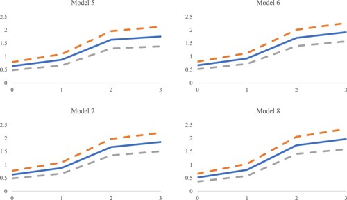
As opposed to the previous studies employing this methodology, the number of cross-sections is quite high whereas the time horizon is only five years. Therefore, to estimate the autoregressive coefficients directly at each h-step-ahead, we lose 20% of our entire sample for each step further. Hence, we note that the interpretation of the results after horizon h = 1 requires a precautionary approach because impulse responses estimated by LP can be severely biased with small sample sizes, as indicated by Herbst and Johannsen (2021).

6. CONCLUSIONS

This paper shows that the internal mobility of the Australian population has a local economic impact because migration flow pushes up the demand for housing in destination areas and leads to an increase in house prices. Using disaggregated SA3-level data on annual internal migration flows and annual changes in house prices for 237 regions in Australia, we find that migration that amounts to 1% of the initial local area population is associated with a 0.52% to 0.71% increase in house prices across different empirical specifications. We also find that migration inflow delivers a significant positive effect on house prices in metropolitan areas such as Sydney and Melbourne but is much less driver in non-metropolitan areas in Australia.

In recent years, property market experts have made the argument that internal migration away from Australia’s big cities has caused house prices to increase in regional cities or suburbs. Our empirical findings, in contrast, provide sufficient evidence for rejecting this argument by indicating that internal migration pushes up housing prices in metropolitan areas rather than non-metropolitan or regional areas.

Overall, the results provide valuable insights into the local housing markets and their role in sustainable economic development. Local economic development is, for the most part, achieved by attracting newcomers to the cities/towns and completed through the participation of migrants in local labour markets and their involvement in local housing markets. Given that house prices are an essential source of human capital accumulation and play an important role in fuelling the growth of economies, it could be argued that internal migration and its positive influence on local housing markets play a crucial role in fostering the local and regional economic development in Australia. New housing policies that aim to achieve a suitable housing supply both for the existing migrants (e.g., workers and professionals) and the potential migrants can significantly contribute to the success of local economic development. It is worth emphasizing that some regions within the coastal cities of the Gold Coast, the Sunshine Coast and the greater city of Brisbane in Queensland have attracted high numbers of internal migrants over the past years. A similar pattern has been observed in Victoria (Wyndham, Melbourne City and Casey-South) and New South Wales (Sydney Inner City, Parramatta and Campbelltown). The persistent inter- and intra-state migration to these areas needs to be examined further, that is, the main characteristics, motivations of migrants and the related new housing policies, in order to achieve sustainable population distribution and strengthen local economic development in Australia.

ACKNOWLEDGEMENTS

We thank the editors and three anonymous reviewers for their careful reading of the manuscript and thoughtful comments. We also thank our colleagues, Murat Guray Kirdar and Bernd Hayo, for their assistance and constructive feedback. An earlier version of this paper was circulated via the MAGKS Joint Discussion Papers in Economics series and presented at a poster session of the 2022 American Economic Association Meeting, and seminars at the Queensland University of Technology, University of Reading, and Universität zu Koln. We assume full responsibility for any mistakes or omissions that may have remained inadvertently in the paper.

DISCLOSURE STATEMENT

No potential conflict of interest was reported by the authors.

Additional information

Funding

The authors thank the Queensland University of Technology for financing the interstate migration data purchased from the Australian Bureau of Statistics (ABS).

Notes

1. Bernard et al. (2017) showed that Australia exhibits the highest level of residential mobility among the 16 countries (Australia, the United States and 14 European countries), with an average of 5.1 moves per individual.

2. On 30 June 2019, the total value of residential dwellings in Australia was A$6720 billion (as of March 2020, this figure was A$7237 billion). New South Wales, Victoria and Queensland had 40%, 28%, and 15%, respectively, of residential dwelling stock value (ABS 6416.0, tab. 6: Value of residential dwellings).

3. According to the World Economic Forum (WEF) (2017), there are 244 million international migrants and 763 million internal migrants worldwide based on 2015 and 2013 data, respectively.

4. Whilst Glaeser and Gyourko (2005) showed that areas with low housing prices tend to exhibit human accumulation and regional economic declines, Miller et al. (2011) found that house price changes have significant effects on local gross metropolitan product in the United States.

5. For the related property industry reports, see https://www.smartrepm.com.au/2019/10/investors-internal-migration-drives-house-prices/; and https://a-d.com.au/buying-living/market-insights/how-australias-internal-migration-is-affecting-housing-prices/.

6. We are aware that the impact of internal migration on house prices without controlling for international migrants could be not only due to internal migrants but also, at least partly, an effect due to international migrants moving to similar places as internal migrants. However, data on international migration flows are not available for SA3-level small areas. Furthermore, the previous research found that a 1% increase in local population due to immigration increases home prices in Australia by 0.7–0.9% per year, but only in significant urban areas (Moallemi et al., 2021; Moallemi & Melser, 2020). Since the focus has been in urban areas, the overall effect of immigrants on housing prices could even be smaller than reported.

7. Saiz (2003) examined the impact of an exogenous immigration shock after the Mariel boatlift on changes in rental prices in Miami. This exogenous immigration shock added an extra 9% to Miami’s renter population in 1980.

8. We are also aware of the fact that the way housing markets adjust when houses differ in terms of their quality is essential. However, we do not have the appropriate data (e.g., the size and quality of dwellings) at the SA3 level to estimate models with different housing quality levels.

9. We used alternative base years of 2008 and 2009 in the IV construction and ran our regressions accordingly as a further robustness check. Our results are insensitive to the exercise of selecting alternative base years and are available from the authors upon request.

10. The rest of the variables are as described as in equation (1).

11. The first-stage coefficients are also in line with the findings of Sá (2015), who estimated a first-stage coefficient of 0.9.

12. To provide a further robustness check, we also controlled for labour force participation rate and ended up with similar results – an imperceptibly smaller coefficient – which is available from the authors upon request.

13. Using another interaction variable that represents all three Greater Capital Cities of Sydney, Melbourne and Brisbane, we find that the $\beta$-coefficient is 0.525 and significant at the 1% level, and that migration inflow in all capital cities leads to an annual increase of 0.12% in house prices.

14. Previous literature has estimated negative impacts of immigration (Accetturo et al., 2014; Sá, 2015; Saiz & Wachter, 2011), and internal migration (Stillman & Maré, 2008) on average house prices/rents, mainly when focusing on small local areas – which again confirms our findings. In these studies, the displacement of natives from migration-receiving areas is the main explanation of the negative impact. However, as our dataset does not allow us to identify the native versus foreign-born residents’ migration flows, we cannot analyse the separate impact of native displacement.

15. Another way to check for robustness could be parallel pre-trend analysis (as provided by Goldsmith-Pinkham et al., 2020, p. 2620, fig. 3); however, we cannot conduct it as our dependent variable is not available before 2014.

REFERENCES

- Accetturo, A., Manaresi, F., Mocetti, S., & Olivieri, E. (2014). Don’t stand so close to me: The urban impact of immigration. Regional Science and Urban Economics, 45, 45–56. https://doi.org/10.1016/j.regsciurbeco.2014.01.001
- Akbari, A. H., & Aydede, Y. (2012). Effects of immigration on house prices in Canada. Applied Economics, 44(13), 1645–1658. https://doi.org/10.1080/00036846.2010.548788
- Aydemir, A., & Borjas, G. J. (2011). Attenuation bias in measuring the wage impact of immigration. Journal of Labor Economics, 29(1), 69–112. https://doi.org/10.1086/656360
- Bell, M., Charles-Edwards, E., Ueffing, P., Stillwell, J., Kupiszewski, M., & Kupiszewska, D. (2015). Internal migration and development: Comparing migration intensities around the world. Population and Development Review, 41(1), 33–58. https://doi.org/10.1111/j.1728-4457.2015.00025.x
- Bell, M., & Cooper, J. (1995). Internal migration in Australia 1986–1991: The overseas-born. Australian Government Publishing Service.
- Bell, M., & Hugo, G. (2000). Internal migration in Australia: 1991–1996 overview and the overseas-born. Department of Immigration and Multicultural Affairs.
- Bernard, A., Forder, P., Kendig, H., & Byles, J. (2017). Residential mobility in Australia and the United States: A retrospective study. Australian Population Studies, 1(1), 41–54. https://doi.org/10.37970/aps.v1i1.11
- Borusyak, K., Hull, P., & Jaravel, X. (2021). Quasi-experimental shift–share research designs. Review of Economic Studies, 89(1), 181–213. https://doi.org/10.1093/restud/rdab030
- Burnley, I. H. (1996). Associations between overseas, intra-urban and internal migration dynamics in Sydney, 1976–91. Journal of the Australian Population Association, 13(1), 47–66. https://doi.org/10.1007/BF03029321
- Burnley, I. H., Marshall, N., Murphy, P. A., & Hugo, G. J. (2007). Housing factors in welfare migration to and from metropolitan cities in Australia. Urban Policy and Research, 25(3), 287–304. https://doi.org/10.1080/08111140701541180
- Cameron, G., Muellbauer, J., & Murphy, A. (2006). Housing market dynamics and regional migration in Britain. https://econpapers.repec.org/paper/cprceprdp/5832.htm
- Cannari, L., Nucci, F., & Sestito, P. (2000). Geographic labour mobility and the cost of housing: Evidence from Italy. Applied Economics, 32(14), 1899–1906. https://doi.org/10.1080/000368400425116
- Champion, T., Cooke, T., & Shuttleworth, I. (Eds.). (2017). Internal migration in the developed world: Are we becoming less mobile? Routledge.
- Charles-Edwards, E., Bell, M., Cooper, J., & Bernard, A. (2018). Population shift: Understanding internal migration in Australia, 2071.0 Census of Population and Housing: Reflecting Australia – stories from the Census, 2016, Australian Bureau of Statistics (ABS).
- Coleman, A., & Landon-Lane, J. (2007). Housing markets and migration in New Zealand, 1962–2006 (No. DP2007/12). Reserve Bank of New Zealand.
- Cooke, T. J., Mulder, C. H., & Thomas, M. (2016). Union dissolution and migration. Demographic Research, 34, 741–760. https://doi.org/10.4054/DemRes.2016.34.26
- Das, M., de Valk, H., & Merz, E. M. (2017). Mothers’ mobility after separation: Do grandmothers matter? Population, Space and Place, 23(2), e2010. https://doi.org/10.1002/psp.2010
- Degen, K., & Fischer, A. M. (2017). Immigration and Swiss house prices. Swiss Journal of Economics and Statistics, 153(1), 15–36. https://doi.org/10.1007/BF03399433
- Dowling, H. (2019). Market growth expected for regional Australia – Smart property investment. https://www.smartpropertyinvestment.com.au/buying/19875-market-growth-expected-for-regional-australia
- Favara, G., & Imbs, J. (2015). Credit supply and the price of housing. American Economic Review, 105(3), 958–992. https://doi.org/10.1257/aer.20121416
- Forster, C. (2006). The challenge of change: Australian cities and urban planning in the new millennium. Geographical Research, 44(2), 173–182. https://doi.org/10.1111/j.1745-5871.2006.00374.x
- Fratesi, U., & Percoco, M. (2014). Selective migration, regional growth and convergence: Evidence from Italy. Regional Studies, 48(10), 1650–1668. https://doi.org/10.1080/00343404.2013.843162
- Gabriel, S. A., Shack-Marquez, J., & Wascher, W. L. (1992). Regional house-price dispersion and interregional migration. Journal of Housing Economics, 2(3), 235–256. https://doi.org/10.1016/1051-1377(92)90002-8
- Ghourchian, S., & Yilmazkuday, H. (2020). Government consumption, government debt and economic growth. Review of Development Economics, 24(2), 589–605. https://doi.org/10.1111/rode.12661
- Glaeser, E. L., & Gyourko, J. (2005). Urban decline and durable housing. Journal of Political Economy, 113(2), 345–375. https://doi.org/10.1086/427465
- Glitz, A. (2012). The labor market impact of immigration: A quasi-experiment exploiting immigrant location rules in Germany. Journal of Labor Economics, 30(1), 175–213. https://doi.org/10.1086/662143
- Goldsmith-Pinkham, P., Sorkin, I., & Swift, H. (2020). Bartik instruments: What, when, why, and how. American Economic Review, 110(8), 2586–2624. https://doi.org/10.1257/aer.20181047
- Gonzalez, L., & Ortega, F. (2013). Immigration and housing booms: Evidence from Spain. Journal of Regional Science, 53(1), 37–59. https://doi.org/10.1111/jors.12010
- Greenwood, M. J., & Hunt, G. (1984). Migration and interregional employment redistribution in the United States. American Economic Review, 74(5), 957–969. https://www.jstor.org/stable/555
- Hatton, T. J., & Tani, M. (2005). Immigration and inter-regional mobility in the UK, 1982–2000. The Economic Journal, 115(507), F342–F358. https://doi.org/10.1111/j.1468-0297.2005.01039.x
- Helderman, A., Mulder, C. H., & Van Ham, M. (2004). The changing effect of home ownership on residential mobility in the Netherlands, 1980–98. Housing Studies, 19(4), 601–616. https://doi.org/10.1080/0267303042000221981
- Herbst, E., & Johannsen, B. K. (2021). Bias in local projections (FEDS Working Paper No. 2020-010R1). https://ssrn.com/abstract=3600410
- Howard, G., & Liebersohn, J. (2021). Why is the rent so darn high? The role of growing demand to live in housing-supply-inelastic cities. Journal of Urban Economics, 124, 103369. https://doi.org/10.1016/j.jue.2021.103369
- Jarvie, W. K. (1989). Changes in internal migration in Australia: Population or employment-led? In L. J. Givson & R. J. Stimson (Eds.), Regional structure and change, experiences and prospects in two mature economies (Monograph Series No. 8, pp. 47–60). Regional Science Research Institute.
- Jeanty, P. W., Partridge, M., & Irwin, E. (2010). Estimation of a spatial simultaneous equation model of population migration and housing price dynamics. Regional Science and Urban Economics, 40(5), 343–352. https://doi.org/10.1016/j.regsciurbeco.2010.01.002
- Jordà, Ò. (2005). Estimation and inference of impulse responses by local projections. American Economic Review, 95(1), 161–182. https://doi.org/10.1257/0002828053828518
- Jud, G. D., Benjamin, J. D., & Sirmans, G. S. (1996). What do we know about apartments and their markets? Journal of Real Estate Research, 11(3), 243–257. https://doi.org/10.1080/10835547.1996.12090826
- Kalemba, S. V., Bernard, A., Charles-Edwards, E., & Corcoran, J. (2020). Decline in internal migration levels in Australia: Compositional or behavioural effect? Population, Space and Place, 27(7). https://doi.org/10.1002/psp.2341
- Kemper, F. J. (2004). Internal migration in Eastern and Western Germany: Convergence or divergence of spatial trends after unification? Regional Studies, 38(6), 659–678. https://doi.org/10.1080/003434042000240969
- Koo, B., Lee, S., & Seo, M. (2020). Identification and estimation of heterogeneous dynamic causal effects using local projection instrumental variable. https://econ.wisc.edu/wp-content/uploads/sites/89/2020/11/draft_KLS_Nov30-2020.pdf
- Kubis, A., & Schneider, L. (2016). Regional migration, growth and convergence – A spatial dynamic panel model of Germany. Regional Studies, 50(11), 1789–1803. https://doi.org/10.1080/00343404.2015.1059932
- Ley, D. (2007). Countervailing immigration and domestic migration in gateway cities: Australian and Canadian variations on an American theme. Economic Geography, 83(3), 231–254. https://doi.org/10.1111/j.1944-8287.2007.tb00353.x
- Miller, N., Peng, L., & Sklarz, M. (2011). House prices and economic growth. Journal of Real Estate Finance and Economics, 42(4), 522–541. https://doi.org/10.1007/s11146-009-9197-8
- Moallemi, M., & Melser, D. (2020). The impact of immigration on housing prices in Australia. Papers in Regional Science, 99(3), 773–786. https://doi.org/10.1111/pirs.12497
- Moallemi, M., Melser, D., Chen, X., & De Silva, A. (2021). The globalization of local housing markets: Immigrants, the motherland and housing prices in Australia. Journal of Real Estate Finance and Economics, 65(1), 103–126. https://doi.org/10.1007/s11146-021-09828-2
- Molloy, R., Smith, C. L., & Wozniak, A. (2011). Internal migration in the United States. Journal of Economic Perspectives, 25(3), 173–196. https://doi.org/10.1257/jep.25.3.173
- Mulder, C. H., & Cooke, T. J. (2009). Family ties and residential locations. Population, Space and Place, 15(4), 299–304. https://doi.org/10.1002/psp.556
- Mulhern, A., & Watson, J. G. (2009). Spanish internal migration: Is there anything new to say? Spatial Economic Analysis, 4(1), 103–120. https://doi.org/10.1080/17421770802625841
- Østbye, S., & Westerlund, O. (2007). Is migration important for regional convergence? Comparative evidence for Norwegian and Swedish counties, 1980–2000. Regional Studies, 41(7), 901–915. https://doi.org/10.1080/00343400601142761
- Ozgen, C., Nijkamp, P., & Poot, J. (2010). The effect of migration on income growth and convergence: Meta-analytic evidence. Papers in Regional Science, 89(3), 537–561. https://doi.org/10.1111/j.1435-5957.2010.00313.x
- Palomares-Linares, I., & Van Ham, M. (2020). Understanding the effects of homeownership and regional unemployment levels on internal migration during the economic crisis in Spain. Regional Studies, 54(4), 515–526. https://doi.org/10.1080/00343404.2018.1502420
- Pettersson, A., & Malmberg, G. (2009). Adult children and elderly parents as mobility attractions in Sweden. Population, Space and Place, 15(4), 343–357. https://doi.org/10.1002/psp.558
- Rowland, D. T. (1979). Internal migration in Australia (No. 1). Australian Bureau of Statistics (ABS).
- Sá, F. (2015). Immigration and house prices in the UK. The Economic Journal, 125(587), 1393–1424. https://doi.org/10.1111/ecoj.12158
- Saiz, A. (2003). Room in the kitchen for the melting pot: Immigration and rental prices. Review of Economics and Statistics, 85(3), 502–521. https://doi.org/10.1162/003465303322369687
- Saiz, A. (2007). Immigration and housing rents in American cities. Journal of Urban Economics, 61(2), 345–371. https://doi.org/10.1016/j.jue.2006.07.004
- Saiz, A., & Wachter, S. (2011). Immigration and the neighborhood. American Economic Journal: Economic Policy, 3(2), 169–188. https://doi.org/10.1257/pol.3.2.169
- Sanchis-Guarner, R. (2017). Decomposing the impact of immigration on house prices (IEB Working Paper No. 2017/14). https://ssrn.com/abstract=3091217 or http://doi.org/10.2139/ssrn.3091217
- Shearer, H., & Burton, P. (2019). Towards a typology of tiny houses. Housing, Theory and Society, 36(3), 298–318. https://doi.org/10.1080/14036096.2018.1487879
- Silverstein, M., & Giarrusso, R. (2010). Aging and family life: A decade review. Journal of Marriage and Family, 72(5), 1039–1058. https://doi.org/10.1111/j.1741-3737.2010.00749.x
- Simon-Davies, J. (2018). Population and migration statistics in Australia. Department of Parliamentary Services, Parliamentary Library.
- Stillman, S., & Maré, D. C. (2008). Housing markets and migration: Evidence from New Zealand. SSRN 1146724.
- Stock, J. H., & Yogo, M. (2005). Testing for weak instruments in linear IV regression. In Identification and inference for econometric models: Essays in honor of Thomas Rothenberg. https://ssrn.com/abstract=1734933
- Thomas, M. J. (2019). Employment, education, and family: Revealing the motives behind internal migration in Great Britain. Population, Space and Place, 25(4), e2233. https://doi.org/10.1002/psp.2233
- Tyrcha, A. (2020). Migration and housing markets-evidence from Sweden (Doctoral dissertation). University of Cambridge.
- Vermeulen, W., & Van Ommeren, J. (2009). Does land use planning shape regional economies? A simultaneous analysis of housing supply, internal migration and local employment growth in the Netherlands. Journal of Housing Economics, 18(4), 294–310. https://doi.org/10.1016/j.jhe.2009.09.002
- Wang, X. R., Hui, E. C. M., & Sun, J. X. (2017). Population migration, urbanization and housing prices: Evidence from the cities in China. Habitat International, 66, 49–56. https://doi.org/10.1016/j.habitatint.2017.05.010
- World Economic Forum (WEF). (2017). Migration and its impact on cities (Report No. REF 061017, October). https://www3.weforum.org/docs/Migration_Impact_Cities_report_2017_low.pdf
- Wozniak, A., & Murray, T. J. (2012). Timing is everything: Short-run population impacts of immigration in US cities. Journal of Urban Economics, 72(1), 60–78. https://doi.org/10.1016/j.jue.2012.03.002
- Zabel, J. E. (2012). Migration, housing market, and labor market responses to employment shocks. Journal of Urban Economics, 72(2–3), 267–284. https://doi.org/10.1016/j.jue.2012.05.006