The composition of local government expenditure and income growth: the case of Sweden

ABSTRACT

This paper analyses the relationship between the composition of local government expenditure and income growth rate at the local level. Based on a panel of municipality-level data for Sweden spanning the period 1996–2015, we find indications of a negative relative ‘growth effect’ of education spending compared with both perceived non-productive expenditure shares and childcare and infrastructure spending, both viewed as productive. However, the robustness of these results is challenged when considering spatial interactions, and the choice of panel construction to address reverse causality. To some extent the results are confined to the assumption that local fiscal policy is exogenous.

KEYWORDS:

• composition
• expenditure
• growth
• local governments
• spatial econometrics

JEL:

• H70
• O40
• R10

1. INTRODUCTION

In 2020, the average share of general government spending in gross domestic product (GDP) for industrialized countries was approximately 50%. Whether public policy has implications for economic growth has long been at the core of research in public finance. In an endogenous growth model, Barro (1990) theoretically shows that the growth rate initially increases with productive government tax-financed expenditure, while unproductive government expenditure has a negative growth effect. Empirical results using cross-country data confirm the presence of such absolute productivity effects, that is, that the long-run growth rate is negatively affected by taxes while productive government expenditure enhances growth (e.g., Bleaney et al., 2001; Alfonso & Gonzáles Alegre, 2011; and the surveys by Poot, 2000; and Nijkamp & Poot, 2004). Though, as demonstrated by Devarajan et al. (1996), it is important to distinguish between absolute productivity and relative productivity of spending components, as overspending on public services that are traditionally viewed as (absolute) productive may turn out to have negative growth effects in relative terms.

Decentralization in many Organisation for Economic Co-operation and Development (OECD) countries has led to an increase in both the size and importance of regional- and local-level governments for economic activity. There is a large literature examining whether fiscal decentralization has any effect on growth, where studies by, for example, Ligthart and van Oudheusden (2017) and Carniti et al. (2019) show support for such a positive growth effect. In this paper, the relationship between local government spending pattern and economic growth is in focus. More precisely, we estimate the association between the income growth rate at the local level and reallocations of expenditure between functional areas of local governments, using Swedish municipality-level data. To the best of our knowledge this is still a rather scarcely explored area, especially the relative importance for various public sector budget components at the subnational level.

Though the empirical literature on the importance of public finance in an endogenous growth setting is vast, we aim to contribute to the literature in at least three ways. First, we study growth effects at the subnational (local) level of changing the composition of local government operational expenditure, that is, the relative importance of different spending categories. An important benefit of using data for a specific country is that we decrease some of the apparent measurement errors present in cross-country studies. Further, most studies based on subnational level data mainly focus on tax-financed higher (absolute) productive spending (e.g., Helms, 1985, and Bania et al., 2007 using US state-level data; and Shaltegger & Torgler, 2006, using state- and local-level Swiss data) while our identification follows the tradition of Devarajan et al. (1996) and comes from time variation in spending shares as result of rebalancing the local government budget (relative productivity), keeping the budget constant. In this sense our study is closely related to Yilmaz (2018) who uses province-level panel data from Turkey, but focuses on growth effects of public investments, while we use current spending. Our analysis is based on a panel of Swedish municipality-level data over the period 1996–2015, where growth is measured in terms of personal income. Sweden is here an interesting case study. As in many other Organisation for Economic Co-operation and Development (OECD) countries there was a general pressure on the Swedish economy during the 1990s, which had implications for public policy and fiscal decentralization. In 1995, Sweden also became a member of the European Union (EU). During this same time the increased knowledge about the importance of the local and regional levels for competitiveness of firms and growth triggered more and more local councils to set own growth objectives. Swedish municipalities also have considerable autonomy, which means that there are rather large degrees of freedom to which they can reallocate between spending areas. The analysis presented here is also relevant from a more general policy perspective, even in the absence of local growth objectives. If government spending at subnational levels is associated with growth as suggested in the decentralization literature, a task for local and regional councils should be to identify not only absolute but also potentially relative productive spending which can be captured by a reallocation of a fixed budget and render a growth-enhancing effect.

Second, much of the recent debate in the empirical literature on whether the composition of government spending matters for growth has revolved around (1) the importance of including the full budget option to avoid misleading results (Kocherlakota & Yi, 1997; Kneller et al., 1999; Bleaney et al., 2001; Gemmell et al., 2016; Chu et al., 2020), and (2) reverse causality. In contrast to Yilmaz (2018) who also uses subnational level data but following recent empirical cross-country studies we include the full budget option. The reverse causality issue has to a large extent been addressed by taking the average over usually a five-year period to decrease business-cycle-like effects of fiscal policy. We follow Chu et al. (2020) and compare results based on the traditional averaging as opposed to using five-year forward-moving averages of all variables. Since this does not fully handle problems with endogeneity, robustness testing using the generalized method of moments (GMM) estimator is discussed.

Third, we contribute by also handling spatial effects, using spatial econometrics to control for the absorption capacity of local labour market. Most studies in this line of research have ignored distortions in terms of potential external effects on the income and/or expenditure side. Horizontal tax competition is an example of such an externality, which means that tax changes of one locality affects tax income of another locality due to mobility of the tax base.¹ Another example is spillover effects of public investments, which, as noted by Munnell (1992), potentially are larger for small regions but rarely explicitly modelled. Thus, failing to control for spatial interactions may lead to biased and inconsistent results. Spatial interactions have previously proven to be of importance in studies using Swedish local-level growth-migration data (Lundberg, 2003, 2006) and US county-level growth-inequality data (Atems, 2013).

The remainder of the paper is structured as follows. The next section provides a brief literature review. Section 3 presents the empirical specification and econometric methodology. Section 4 presents the data, a brief overview of the institutional background of the public sector in Sweden and preliminary unconditional results. The results of the econometric analysis are presented in Section 5 and discussed in Section 6, which also contains concluding remarks.

2. BRIEF LITERATURE REVIEW

The empirical literature on public finance and economic growth exploded in the 1990s after the development of the endogenous growth model by Romer (1986), Lucas (1988) and Barro (1990). Helms (1985) is one of the first studies to specifically separate out the growth effects of various spending components of the subnational government. His results, based on US state-level panel data, indicate that state and local tax increases slow down economic growth if revenue is used for transfer payments. However, the negative effect of a higher tax may be counterbalanced if the local government uses revenue to finance improved publicly provided services, for example, education and infrastructure. The impact of taxation on growth may, however, vary depending on the initial tax rate, where the growth-enhancing productivity effect may be largest for low initial tax rates and the crowding-out effect dominates for higher tax rates (Glomm & Ravikumar, 1997; Poot, 2000; Jaimovich & Rebelo, 2017).

The strand of the growth literature focusing on effects of changes in the relative amount of expenditure is less vast than the one focusing on growth and taxation, and mainly lean on the theoretical framework by Devarajan et al. (1996). Government expenditure is viewed as either productive, $g_1$, or non-productive, $g_2$. Devarajan et al. point out that the condition for a shift in the composition of government expenditure to enhance growth depends on both the productivity in absolute terms of $g_1$ and $g_2$ as indicated by their respective distribution parameter $\beta$ and $\gamma$ in the production function, and their respective initial spending shares $\phi$ and $(1-\phi )$. This means that even though $\beta >\gamma$ increasing productive spending further can have a negative growth effect if the initial spending share is too high. Note that long-run growth in this case can be enhanced by changing the composition of expenditure with constant total expenditure. A benefit of the Devarajan et al. framework is that it is rather general and allows for, for example, inclusion of capital (investment) and/or current spending, which in turn may be disaggregated.

Most empirical studies in this strand are based on cross-country data on developing countries, OECD countries, or a mix of developing and developed countries (e.g., Devarajan et al., 1996; Kneller et al., 1999; Bleaney et al., 2001; Ghosh & Gregoriou, 2008; Gemmell et al., 2016; Acosta-Ormaechea & Morozumi, 2017; Chu et al., 2020), some country case studies at the national level usually based on time-series data (Cullison, 1993 for the United States; Singh & Weber, 1997, and Colombier, 2011, for Switzerland; Olabisi & Oloni, 2012, for Nigeria; and Bojanic, 2013, for Bolivia), and fewer studies using subnational level-panel data (Yilmaz, 2018). Based on data for developing countries Devarajan et al. (1996) and Ghosh and Gregoriou (2008) find that current (capital) spending has a positive (negative) relationship with growth. Devarajan et al. say that this perhaps surprising result may be explained by overspending on expenditure categories that are traditionally claimed to be growth enhancing (capital spending), or in the optimal fiscal policy perspective in Ghosh and Gregoriou that spending categories that are traditionally perceived as productive in the production function are not so in reality or have simply not generated the expected productivity. Chu et al. (2020) challenge these results and find that a statistically significant relationship is only established when controlling for the full budget constraint, which was not the case in Devarajan et al. (1996). Gemmell et al. (2016), Acosta-Ormaechea and Morozumi (2017) and Yilmaz (2018) find a positive effect on growth of reallocation towards education spending. The result on infrastructure spending is, however, less decisive. The general results in the country case studies confirm these findings.

3. EMPIRICAL SPECIFICATION AND METHODOLOGY

We start this section by presenting the regression model and interpretation of the municipality fiscal variables in terms of compositional effects. We then motivate the spending shares that we focus on and continue with explaining other control variables. Subsection 3.2 then presents a discussion on identification and causality, and subsection 3.3 contains a discussion on spatial interactions and choice of econometric estimator.

3.1. The estimation equation

The empirical analysis is based on the following reduced-form equation, where the average annual income growth rate between time t – T and t for individuals in municipality i, $y_{i,t}$, is assumed to depend on the local government fiscal variables, that is, expenditure (X) and revenue (R), two-way fixed effects (municipality-specific effects ${\chi }_i$, and time-specific effects ${\delta }_t$), the initial income level (Y), spatial dependence $(\mathit{W}\times y)$, other control variables included in the vector Z, and an error term $({\epsilon }_{it})$. (1) $y_{i,t}=a_1{Y}_{i,t-T}+a_2{\mathit{W}}_{i,t}\times y_{j,t-T}+\sum _{s=1}^l{A}_s^X{X}_{i,s,t-T}+\sum _{s=1}^r{A}_s^R{R}_{i,s,t-T}+A_3{\mathit{Z}}_{i,t-T}+{\chi }_i+{\delta }_t+{\epsilon }_{i,t}$(1) In contrast to the standard approach in the Barro-inspired empirical endogenous growth literature where the fiscal variables are divided by income, we hold total expenditure and total revenue constant, respectively, in accordance with Devarajan et al. (1996) to focus on the composition of expenditure. By re-defining the expenditure and revenue side of the local government budget constraint, as expenditure shares, $X_{i,s,t-T}=g_{i,s,t-T}/T{E}_{i,t-T}$, and revenue shares, $R_{i,s,t-T}=re{v}_{i,s,t-T}/T{R}_{i,t-T}$, we have: (2) $\sum _{s=1}^x{X}_{i,s,t-T}=1\mathrm{and}\sum _{s=1}^r{R}_{i,s,t-T}=1$(2) Thus, one of the fiscal variables on the expenditure side and revenue side, respectively, must be omitted to avoid perfect collinearity. The choice of omitted variables will affect the interpretation of the empirical results, since the omitted expenditure (income) variable is the one assumed to decrease when the other expenditure (income) share increases. However, if identification is correctly specified it should not matter which spending share is omitted, and we can thereby arbitrarily omit one.

In line with Devarajan et al. (1996) and subsequent studies, we make no a priori assumption about whether a certain expenditure category is productive or unproductive. There are, however, results in the literature that identify some channels by which public spending can foster growth. Infrastructure spending is perhaps the most documented growth-enhancing category. A well-functioning infrastructure, facilitated by public infrastructure spending on, for example, roads and broadband, augments physical capital in the production function by promoting productivity (e.g., Aschauer, 1989; Easterly & Rebelo, 1993; Glomm & Ravikumar, 1997). Similarly, Barro (1990) and Glomm and Ravikumar (1997) identify a positive growth-effect of public spending on education through human capital formation. Based on these previous findings we are specifically interested in spending on infrastructure and education to see whether these are relatively more productive than other budget components through a positive correlation with growth facilitated by a compositional reallocation of local government spending. In addition, we will also separate out spending on childcare. The argument is similar as infrastructure, but in this case mainly as an augmentation on labour, in terms of both the labour market participation decision and productivity. The social infrastructure in Scandinavian countries, including publicly financed childcare and elderly care services and parental leave for both women and men, that encourages dual-earner families, has been put forward as an explanation to why the decrease in fertility rate is less steep in these countries compared with other Western economies (Ferrarini, 2003; Löfström, 2009). Kimmel (2006) argues that access to reliable and high-quality childcare facilitates the balance between work and family life and thereby attracts and strengthens labour market participation among individuals who are also parents, not least the participation and retention of female labour (see also Bettio & Plantenga, 2008, for similar arguments for other so-called care systems). Based on Swedish household data, Gustafsson and Stafford (1992) find that access to childcare provided by the municipalities encourages especially female labour market activity. By extension this is of importance for labour development and hence economic growth.²

Thus, a local government spending category is viewed as productive if the corresponding coefficient is positively statistically significant. Since we deal with compositional effects, the interpretation is in terms of relative productivity of the spending category, that is, relative to the omitted budget component which makes the reallocation possible (more output in terms of income growth compared with a unit increase in the other component).

We also include the revenue side of the budget in (1) motivated by Kneller et al. (1999) and Bleaney et al. (2001) who point out that it is important to take the full government budget constraint including debt into account in the estimations, in addition to other standard controls, to avoid omitted variable bias. For instance, Bleaney et al. (2001) include the budget surplus to empirically control for the possibility that governments may fail to balance the budget each period. Public sector debt is affected by government spending decisions and the possibility or capability to raise balancing revenue and can in turn affect the behaviour of firms and households. In Sweden, local governments are, however, only allowed to use debt to finance investments and not current spending. Failure to consider the full budget constraint of the government may lead to inconclusive and biased results as shown by Kocherlakota and Yi (1997), Kneller et al. (1999) and Bleaney et al. (2001). One may argue that this is not applicable to the case of Sweden due to the balanced-budget requirement since the year 2000. However, our data period starts in 1996 and, as indicated in Figure A1 in Appendix A in the supplemental data online, there are quite a few municipalities over the study period with difficulties in reporting a balanced result. For these reasons and to avoid potential bias in the estimated coefficients of the variables of interest, namely the various expenditure shares, we include the revenue side in the estimations.

The estimation equation (1) also includes the (log) income level Y, motivated by previous literature that uses it to test for conditional income convergence, where the income level is expected to have a negative effect on the income growth rate (Barro & Sala-i-Martin, 1992; Aronsson et al., 2001; Lundberg, 2003, 2006; Värja, 2016). As noted by Nijkamp and Poot (2004), the variable is also needed to avoid bias on the coefficient for government expenditure due to correlation between the two variables according to Wagner’s law.

An advantage of using data for a single country, as opposed to cross-country data, is that all municipalities face the same laws, regulations and macro-level shocks. On the other hand, municipalities could be viewed as entities in a common pool, the nation, and to some extent we control for this by including a variable for spatial dependence $(\mathit{W}\times y)$ (see subsection 3.3). Further, we include municipality-specific effects to control for time-invariable specific settings for each locality, as well as time-specific effects and other variables, Z, that control for intra-macro external shocks and policies.

The vector Z contains control variables for municipality i, including the share of high-educated individuals, the share of foreign-born individuals, density and age composition of the population. The vector also contains the county tax rate which is motivated by Aronsson et al. (2000) who find evidence of vertical expenditure interactions between the county and municipalities due to tax base overlap based on Swedish data. Thus, the county tax rate is included in the estimations to control for county-level spending and growth trends which may affect the local growth rate. Total expenditure as a share of income is included to control for size (level) effects of expenditure. The unemployment rate is also included and reflects the probability of not receiving a job in the municipality, which implies that it is expected to be negatively related to the net migration rate. If unemployed individuals move from the municipality to find a job elsewhere, we expect the unemployment rate to be positively related to the average income growth rate.

3.2. Identification and causality

One obvious problem is reverse causality in the relationship between government expenditure and growth, that is, the difficulty in identifying whether the municipality’s spending decision causes growth or rather is based on expectations of future growth. Another possibility is that the municipality may unproportionally change the budget composition over time towards specific spending areas with the purpose to increase future growth. In our model identification of the association between income growth rate and municipality spending shares comes from the time variation in the spending shares as result of a rebalancing of the local government budget. Time variation in spending shares due to unbalanced budget changes may, however, lead to identification problems. Thus, the source of time variation in budget composition is of importance and one way to explore it in our case is to determine the extent to which structural characteristics can explain the spending pattern. The purpose of the cost equalization system is precisely to account for variation in expenditure levels across municipalities based on structural characteristics. This gives, in theory, every municipality the same opportunity to provide its residents with the same level of welfare services. Some of the main variables to explain differences in net operating expenditure are the age structure, density and socio-economic factors (SOU, 2018:74). Thus, such variables are included in the regression to control for structural aspects which may affect the spending composition over time.

To address reverse causality in the original work by Devarajan et al. (1996) the dependent variable was specified as the five-year forward-moving average of the annual per capita GDP growth rate. This strategy aims at eliminating short-run business-cycle-type effects that could be induced by changes in public spending and has also been used in subsequent studies in this strand of literature (e.g., Ghosh & Gregoriou, 2008; Yilmaz, 2018; Chu et al., 2020). An alternative approach is to use five-year non-overlapping growth periods. In this paper we will use both approaches. Non-overlapping growth periods are with our data specified as 1996–2000, 2001–05, 2006–10 and 2011–15, where the dependent variable will be the (geometric) average of annual growth rate of income over each five-year period. In the literature (e.g., Kneller et al., 1999; Bleaney et al., 2001) this approach is often combined with the independent variables also averaged over the same five-year period. Here, we instead follow, for example, Acosta-Ormaechea and Morozumi (2017) and time-set the public spending variables, as well as the other control variables, at the beginning of each growth period, which also reduces serial correlation. With relatively long growth periods, $T=5$, where each period also spans more than one election period, it is less likely that the local government can predict the growth rate and use that information to determine the allocation of budget shares to different functional areas. The drawbacks of using non-overlapping growth periods are that the results may be sensitive to the choice of baseline year, and that the number of time-series observations is greatly reduced. In the alternative specification with a five-year forward-moving average of annual growth rates of income the number of time-series observations increases. In this latter case we also follow Chu et al. (2020) and use a five-year forward-moving average of the fiscal components and other control variables in the estimations, that is, not only the dependent variable. Robust standard errors clustered on municipalities are used in both alternatives to mitigate the problem of serial correlation and heteroscedasticity.

If the municipality fiscal variables are exogenously given, it is straightforward to use ordinary least squares (OLS) with fixed effects to estimate equation (1). However, neither of the approaches of period-averaging discussed above fully resolves the simultaneity problem. A common econometric solution to address endogeneity is to use instrumentation, such as two-stage least squares (2SLS) (instrumental variables – IV) or the GMM technique. Finding appropriate external instruments (relevant and valid, that is, correlated with the endogenous variable and at the same time orthogonal to the error term) is inheritably difficult. The GMM technique circumvents this problem by using lags of the endogenous variables as instruments (internal instruments), which cannot be done with regular fixed-effects IV estimation (Nickell, 1981). System-GMM improves efficiency compared with difference-GMM by also allowing the first differences of IV as instruments (Arellano & Bover, 1995; Blundell & Bond, 1998). However, this comes to the cost of a crucial assumption of no serial correlation. Considering that we analyse municipality-level data, we cannot rule out the presence of autocorrelation, perhaps especially spatial autocorrelation (see subsection 3.3). An additional concern is that our estimation equation includes several potentially endogenous variables – all fiscal variables, initial income level and the spatial interaction term – and a large set of control variables. The number of instruments therefore easily becomes very large, which tends to both overfit the endogenous variables and weaken tests of instrument validity (Roodman, 2009). GMM results will be discussed as a robustness test to OLS estimations.

3.3. Spatial interactions

Previous literature has found evidence of spatial interactions between local governments in Sweden where there is a consistent positive relationship between the growth rate in average income in neighbouring municipalities and the growth rate of municipality i (Lundberg, 2006; Värja, 2016). Neglecting to control for an existing spatial dependence between neighbouring municipalities can lead to biased and inconsistent estimates (Rey & Montouri, 1999). One way to incorporate this spatial dependence in the estimations is to use a weight matrix (Anselin, 1988). In this paper we construct a weight matrix where the weights are based on the inverse distance to neighbouring municipalities, which means that closer neighbours are given a higher weight.³ Since we mainly think of the spatial interaction in terms of job opportunities, we only assign positive weights to municipalities that are included in the same job market region, and all other municipalities have a weight equal to zero.⁴ Anselin (1988) shows that if there is a spatial interaction between municipalities and this is taken into account by a weight matrix, the standard OLS estimates are inconsistent and biased. One way to address this issue is to use the quasi-maximum likelihood estimator (ML) with the fixed effects spatial model. An alternative is to use the IV or GMM estimator. The point estimates are rather stable to the choice of estimator, however, due to the less efficient estimation method of IV compared with maximum likelihood the standard errors are larger when using IV. In the results section we report the results based on the quasi-maximum likelihood estimator when controlling for spatial interactions.

4. DATA, SWEDISH MUNICIPALITIES AND DESCRIPTIVES

This section starts with a presentation of data source, motivation for choice of study period and definition of variables used in the econometric analysis. Subsection 4.2 then gives a brief description of the structure and tasks of the Swedish municipalities and presents descriptive figures of spending patterns and preliminary unconditional results.

4.1. Data

The empirical analysis is based on a balanced dataset of 282 Swedish municipalities over the period 1996–2015. The total number of municipalities has varied over the study period, from 288 in 1995 and 290 municipalities from 2003 onwards. Of the 290 existing municipalities today, we exclude eight.⁵ All data are collected from Statistics Sweden. We restrict the time period back in time for two main reasons: (1) due to the decentralization wave in Sweden during the first half of the 1990s followed by two major reforms of the intergovernmental grant systems in 1993 and 1996 that gave the municipalities higher degrees of freedom regarding how to allocate grants between spending areas; and (2) more municipalities were subject to jurisdictional border changes before 1996 which would render an even further limitation of number of municipalities we could include in the analysis.

When excluding municipalities, we create empty spaces in the spatial weight matrix, which will affect the coefficients of the spatial variables to some degree; not accounting for the missing municipalities’ effects may bias the coefficient for the spatial effect, making the potential spatial effects smaller. We are, however, not interested in interpreting the size of the spatial effect per se but want to control for the effect of it.

The income level $(Y_{it})$ and, thus, the income growth rate $(y_{it})$ are calculated for the population aged 20 and older. By using individuals older than 20 for average income, we try to avoid some of the dependence between age structure and average income, following what has previously been done by Lundberg (2003, 2006) and Aronsson et al. (2001). All monetary variables are deflated by the national consumer price index since there are no regional- or local-level price indices available.

Table A1 in Appendix A in the supplemental data online presents the definition and content of all included variables in the estimations, including the composition of different expenditure shares. Expenditure data refer to operating (current) expenditure and do not include investment (capital formation) expenditure. In the data source, operating expenditure are reported according to major functional spending categories as they show up in the local government budget; general government services, infrastructure, culture and leisure, childcare, education, elderly and disability care, individual and family care, directed activities, business activities, and financial costs. Here we focus on the three categories infrastructure, childcare and education (see subsection 3.1). The shares are calculated by dividing the expenditure of each functional category with total expenditure, which implies that the sum of expenditure shares is equal to one[. Total expenditure is equal to total revenue, and the revenue shares also sum to 1.

4.2. Swedish municipalities and patterns of income growth and spending

In Sweden, the public sector is structured into three levels of government: local governments (municipalities), regional (county) governments and a central (national) government. The main responsibility of the municipalities is to provide education (primary and secondary education), childcare (including pre-school) and care for the elderly, while the regions mainly provide healthcare. Services that all municipalities are required to provide are regulated by the national government. These national regulations are usually expressed in terms of the purpose of a certain type of service or effort and usually constitute a minimum required level. The subnational tiers have, however, considerable autonomy in deciding how to organize activities and allocate resources. They are also free to extend the services beyond this minimum level, in terms of both quantity and quality. Any changes made by the national government that require an increase in the obligation must be combined with a monetary compensation provided through grants, which we control for in the estimations. In addition to providing compulsory services, the municipalities are also free to engage in the provision of, for example, culture, recreation, heating, electricity, parking and support for the local business community. In addition to the decentralization of tasks from the national government, an expansion of voluntary tasks explains the large size of the local level government relative to the overall public sector in Sweden compared with in many other countries.

The subnational governments are only allowed to tax personal income and they set their own tax rates without intervention from the national government. This means that even if the national government imposes obligations on the local governments, the municipality assemblies are free to adjust the local income tax rate and to decide how much to spend on, for example, childcare, education and care for the elderly, which are the three largest functional spending categories for the local governments. Income tax is a proportional tax and the main source of revenue. For the municipalities the income tax revenue as a share of total revenue was approximately 78% during the study period. Other sources of revenue are intergovernmental grants and user fees. There is, however, a large variation across the country, and in some areas intergovernmental grants are almost as important as taxes as a source of income, while five municipalities in the Stockholm region net contribute to the grant system during the study period.

Municipalities and regions face their own budget constraints, with a budget-balance requirement by law since 2000.⁶ As an indication of the budget-balance status among the municipalities, we can look at their reported annual result over the study period. Figure A1 in Appendix A in the supplemental data online shows that the implementation of the law has led to a large drop in the number of municipalities that report a negative result, even though there are still some municipalities that fail to show a positive result. The unweighted average result among these latter municipalities has varied between −297 SEK per capita in 2006 and −2603 SEK per capita in 2013.⁷

Descriptive statistics for all data used in the analysis are reported in Table A2 in Appendix A in the supplemental data online. Table 1 gives a more in-depth description of the main variables of interest. The distribution of the five-year average of the annual growth rate of personal income across time and municipalities varies between 0.8% for the those with the 10% lowest growth rate to 3.5% for those in the top 10% of the distribution. For the spending shares we see a difference that varies between 4 (infrastructure) and 10 (education) percentage points between the bottom and top 10 percentiles. The largest part of the variation in growth rate takes place over time. Regarding the spending shares, there is less pronounced difference in variation in the cross-section and time dimensions.

Table 1. Descriptive statistics of the growth rate and spending shares in Swedish municipalities, 1996–2015

Variable	Percentile					SD		Mean
	10%	25%	50%	75%	90%	Between	Within
Growth rate	0.008	0.013	0.020	0.026	0.035	0.003	0.010	0.020
Personal income	158.82	175.18	197.08	214.15	232.65	24.556	22.17	198.20
Education	0.289	0.308	0.333	0.360	0.387	0.034	0.021	0.335
Childcare	0.085	0.098	0.115	0.136	0.163	0.026	0.015	0.119
Infrastructure	0.050	0.059	0.068	0.078	0.089	0.013	0.010	0.069

Note: Growth rate is calculated as the geometric mean of annual growth in personal income over five-year periods 1996–2000, 2001–05, 2006–10 and 2011–15, while spending shares are initial values at the start of the growth period.

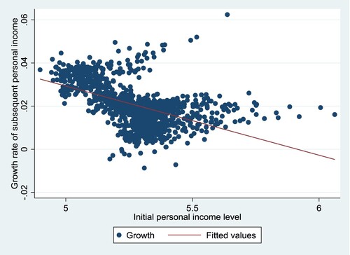
Figure 1 shows the relationship between the initial personal income level and the subsequent growth rate using data for the four growth periods 1996–2000, 2001–05, 2006–10 and 2011–15. It implies a pattern of (unconditional) convergence. However, looking at the separate growth periods indicates that this pattern is not as evident, with periods of divergence especially towards the end of the study period.

Figure 1. Growth rate versus initial (log) personal income level.

Note: Growth rate is calculated as the geometric mean of annual growth of personal income over five-year periods 1996–2000, 2001–05, 2006–10 and 2011–15. Initial personal income is in logarithms.

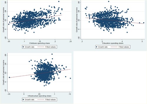
Preliminary unconditional evidence of the relationship between spending shares on education, infrastructure and childcare, and subsequent average personal income growth rate is illustrated in Figure 2. The fitted linear functions indicate a negative relationship with growth for education, and a positive relationship for infrastructure and childcare.

Figure 2. Relationship between initial spending shares and subsequent personal income growth rate.

Note: Growth rate is calculated as the geometric average of annual income growth rate over five-year periods 1996–2000, 2001–05, 2006–10 and 2011–15.

5. RESULTS

Table 2 reports the results of estimating equation (1) with the five-year average of the annual income growth rate at the municipality level as dependent variable. The main variables of interest are the spending shares, where we focus on the spending shares of education, infrastructure and childcare, and thus exclude all other spending categories and treat them as variable. By including the three spending shares in the same regression, we may easily compare their respective relative importance. In all specifications we exclude tax revenue from the model. The estimation strategy is as follows. We first estimate the model using four non-overlapping five-year growth periods with independent variables dated as initial values (columns 1 and 2) and second using five-year forward moving averages of all variables (columns 3 and 4). For both panel structures we show results from excluding (columns 1 and 3) and including (columns 2 and 4) $\mathit{W}\times y_j$ from the estimations, that is, the weight matrix interacted with the income growth rate of surrounding municipalities. In a third step we check the robustness of the results to the definition of spending categories and other additional potentially productive spending components and elaborate on whether the correlations presented in Table 2 also have a causal interpretation.

Table 2. Growth and the composition of municipal spending.

	Five-year non-overlapping growth periods		Five-year forward moving average
	OLS, FE	ML, FE	OLS, FE	ML, FE
	(1)	(2)	(3)	(4)
Childcare	0.027**	0.007	0.021*	0.014
	(0.01)	(0.01)	(0.01)	(0.01)
Education	−0.037***	−0.026***	−0.021**	−0.014
	(0.01)	(0.01)	(0.01)	(0.01)
Infrastructure	0.013	0.009	−0.005	0.008
	(0.02)	(0.01)	(0.02)	(0.02)
Total expenditure	−0.025***	−0.026***	−0.061***	−0.061***
	(0.01)	(0.01)	(0.01)	(0.01)
Other income	0.019**	0.024***	0.070***	0.071***
	(0.01)	(0.01)	(0.01)	(0.01)
Grants & fees	0.020***	0.014**	0.100***	0.087***
	(0.01)	(0.01)	(0.01)	(0.01)
Personal income	−0.083***	−0.072***	0.037***	0.031***
	(0.01)	(0.01)	(0.01)	(0.01)
County tax	0.001	0.005	−0.008**	0.004
	(0.00)	(0.00)	(0.00)	(0.00)
Debt	0.001*	0.000	0.001***	0.001**
	(0.00)	(0.00)	(0.00)	(0.00)
High educated	0.008***	0.005**	0.009***	0.004**
	(0.00)	(0.00)	(0.00)	(0.00)
Foreign born	−0.002	−0.001	−0.001	−0.002
	(0.00)	(0.00)	(0.00)	(0.00)
Unemployment	0.001	0.001	−0.004***	−0.004***
	(0.00)	(0.00)	(0.00)	(0.00)
Aged 0–19	−0.005	−0.000	−0.024***	−0.012**
	(0.01)	(0.00)	(0.01)	(0.01)
Aged 80+	−0.001	0.003	0.005**	0.007***
	(0.00)	(0.00)	(0.00)	(0.00)
Density	−0.004	0.007	−0.018***	−0.008
	(0.00)	(0.00)	(0.00)	(0.00)
_cons	0.541***		0.055
	(0.06)		(0.06)
$W\times y$		0.257***		0.219***
		(0.02)		(0.02)
N	1128	1128	4230	4230
R^2 (within)	0.907	0.910	0.928	0.929
Akaike information criterion (AIC)	−9927.6	−10,065.7	−38,985.3	−39,328.7
Bayesian information criterion (BIC)	−9837.1	−9965.2	−38,801.2	−39,131.9

Note: Dependent variable is the five-year forward moving average of annual growth rate of average personal income. Robust standard errors clustered on municipalities are reported in parenthesis. *, **, ***Significance at the 10%, 5% and 1% levels, respectively. All specifications include both time- and municipality-specific effects. In columns (1) and (2), all explanatory variables use pre-growth period (initial) as the base year; and in columns (3) and (4), all explanatory variables are taken as five-year forward moving averages.

The coefficients on other income and on grants and fees are positively significant, which implies that a shift towards revenue from these sources and away from revenue from distortionary taxation, which is the omitted revenue share, is positively related to growth. A closer look at the different expenditure shares in Table 2 shows that across all specifications the coefficient for infrastructure is never significant. The results for childcare and education are, however, more sensitive to specification. Fully excluding the spatial interaction term increases the point estimates on the local government spending shares in absolute values, and the correlations generally become stronger. If the municipality would decide to change the composition of the budget by reallocating expenditure towards childcare this is positively related to the subsequent local average income growth rate. This result contrasts with the education spending share which is negatively related to the subsequent growth rate. If the municipality would decrease the spending share of education by 1 percentage point, this would relate to a 0.037 percentage point increase in the income growth rate. The results indicate that the budget allocation is not optimum, and there may be room for reallocations to potentially enhance growth.⁸ The result on education spending is stable to controlling for spatial dependence, but only when using non-overlapping growth periods (column 2). Using five-year forward-moving averages and controlling for spatial dependence (column 4) removes all significance for the spending shares. The coefficient on the spatial dependence interaction term is positively significant in both columns (2) and (4), which means that the income growth rates of surrounding municipalities are correlated. As pointed out by Rey and Montouri (1999), this spatial dependence can indicate presence of spillover effects, that is, shocks in one municipality that also affect surrounding municipalities, which potentially may be more important for smaller regions (Munnell, 1992). Not controlling for this spatial interaction will bias the results, and according to Table 2, this is accentuated in combination with the sensitivity of results with respect to how the panel is constructed to iron out business-cycle-like effects.

By comparing the parameter estimates on the spending shares in Table 2, we can determine their respective relative ‘growth effect’. A Wald test shows that the relative ‘growth effect’ of childcare spending is significantly higher than spending on education, and this result is stable across all columns (p-value between 0.000 in column 1 and 0.039 in column 4). There is also a statistically significant difference between spending on education (lower) and infrastructure, but this result is confined to the case of non-overlapping growth periods (p-value between 0.006 in column 1 and 0.015 in column 2). Lastly, we cannot reject the hypothesis of no difference in relative ‘growth effect’ of spending on childcare and infrastructure.

Regarding the results of our control variables⁹ in Table 2, we find, consistent with previous studies on Swedish data (Aronsson et al., 2001; Lundberg, 2003, 2006; Värja, 2016), evidence of conditional convergence indicated by the negatively significant relationship between the average income growth rate and level of average personal income when using non-overlapping growth periods (columns 1 and 2). However, this result is sensitive to the panel construction. When using forward-moving averages (columns 3 and 4), the results instead show a pattern of divergence according to the positively significant coefficient on personal income. Signs of divergence have also been documented in previous studies on regional growth in Sweden for later time periods (Henning et al., 2011; Lundberg, 2006) and in Europe (e.g., Fagerberg & Verspagen, 1996).

The parameter estimate of total expenditure as a share of personal income is negatively statistically significant in all specifications, such as findings by Chu et al. (2020) for both high-income and low- and middle-income countries. This negative level effect of total expenditure suggests that even if the average municipality would increase total current spending with the aim to enhance growth, distortionary effects that arise on the revenue-raising side to balance the budget more than well offset any potential positive effect on growth.¹⁰

There is a robust positive effect of high-educated individuals and the growth rate of personal income. The results on the other control variables are more sensitive to how the panel is constructed, where significance is mostly detected using the five-year forward moving average approach. The level of debt is positively related to the growth rate, and significantly so in columns (3) and (4). Since Swedish municipalities can only use debt to finance investments, this could indicate an expected positive relation between investment and growth. Next, we find that a high unemployment rate negatively affects the growth rate. This negative effect implies that the unemployed stay in the municipality rather than move to find job elsewhere. Also, the age structure of the municipality matters for the growth rate, with a negative effect of a higher share of young (aged 0–19) and a positive effect of a higher share of the population being 80 or older.

5.1. Robustness test: choice of spending components and definition of spending categories

As pointed out by Kneller and Misch (2014) a non-significant coefficient on the spending shares does not necessarily mean that it is of no importance. It could mean that neither the expected productive spending category included in the estimation (childcare, education and infrastructure) nor the expected non-productive excluded categories are indeed productive. However, it could also mean that both are of equal importance, but with opposite signs. Thus, in Tables A3 (non-overlapping growth periods) and A4 (five-year forward moving averages) in Appendix A in the supplemental data online, we check the sensitivity of our results by aggregating the expected productive spending shares (columns 1 and 2) and separating out two additional spending components (columns 3 and 4) to check the sensitivity of results as to which spending components are categorized as productive. Elderly and disability care is motivated by similar arguments as childcare (see subsection 3.1). Approximately 50% of this spending component is devoted to elderly care and 50% to disability care for individuals of all ages. Spending on business activities is a relatively small part of total spending and includes energy, water and waste management, and is also expected to be productive on similar arguments as infrastructure. Note that the variable part of the local government expenditure is equal to the omitted spending share since all shares sum to 1.

According to Tables A3 and A4 in Appendix A in the supplemental data online, where the tax revenue share is omitted in all specifications, similarly as in Table 2, the results are robust to these changes and no additional information can be extracted from collecting the expected productive categories into one. In Table A3, column (4), we detect a positively significant correlation between elderly and disability care and growth. A positive association is expected to the extent that a higher spending share on elderly and disability care facilitates labour market participation and/or productivity. However, as pointed out by an anonymous reviewer, another possibility is a form of attrition considering that one part of the spending component is elderly care, which is mainly directed towards individuals above the age of 80. A combination of low income (retirement payments) and a high death rate for this age group implies a natural increase in the average level of income over the growth period. Therefore, in addition to controlling for the age structure in the estimations, we re-estimate the specifications restricting the income variable to include only income for the population aged 20–64 (see columns 5 and 6 in Tables A3 and A4 in Appendix A in the supplemental data online). The coefficient for elderly and disability spending share is no longer statistically significant, which indicates that the result is both sensitive to the choice of panel construction and to which age groups are included in the income variable. With the age-income restriction we also note that the education share now appears sensitive to the choice of panel construction. The results in Tables A3 and A4 are, however, reassuring in the sense that identification seems to be correctly specified since the results for the control variables are not affected by which spending share is omitted.

Does the choice of denominator for local government expenditure categories matter for the results? In this paper we follow the work initiated by Devarajan et al. (1996) and argue that there is a difference between absolute and relative productive effects of public spending, that can be emphasized using total expenditure as the denominator for the spending categories instead of expressing them in per capita or per income terms. Table A5 in Appendix A in the supplemental data online presents the results of similar specifications as in Table 2, but with the spending shares instead expressed in per capita terms. The results are robust to the choice of denominator, though with generally lower point estimates in absolute values.

5.2. Robustness test: endogeneity

An obvious concern is whether the results presented so far have a causal interpretation. We have therefore rerun the regressions using the dynamic panel system-GMM estimator (Arellano & Bover, 1995; Blundell & Bond, 1998). The choice of dynamic modelling is based on previous results by Bleaney et al. (2001) who find a significant impact of lagged growth.¹¹ The second lag of the dependent variable is also included to control for possible AR(2) as indicated based on tests for serial correlation. To limit the number of instruments we have restricted the lag length presenting results in Table A6 in Appendix A in the supplemental data online using either lags 3–4 or 4–6 to test the robustness of results. As expected, the Hansen J-test for the validity of the full instrument set is sensitive to the number of instruments included and is of concern especially in the case where we control for spatial interaction. The negative significant relation between growth and a reallocation towards education spending remains robust but with slightly higher point estimates than the fixed effects results in Table 2 (columns 3 and 4). Based on this, endogeneity bias does not seem to be of major concern. Since validity tests are questionable when including spatial interactions, the evidence is not enough to support such an interpretation in this case. In line with Bleaney et al. (2001), Bose et al. (2007) and Chu et al. (2020) the first-order autoregressive coefficient (lagged growth) is strongly statistically significant, and the size implies high persistence.

6. DISCUSSION AND CONCLUSIONS

Using Swedish municipality-level data for 1996–2015, the purpose of this paper was to estimate the association between income growth at the local level and a reallocation of expenditure between main functional areas of local governments. By fixing the different shares of expenditure we keep the budget constant and are hence able to evaluate effects of re-distributions of the budget within the local governments, which means that even though a certain spending area is productive in absolute terms and growth-enhancing per se, it may be relatively more productive (render higher output in terms of income growth) to direct the government expenditure towards some other spending category.

In contrast to previous studies by, for example, Gemmell et al. (2016), Acosta-Ormaechea and Morozumi (2017) and Yilmaz (2018) our findings show a negative association between growth and a reallocation from expenditure on perceived non-productive publicly provided services/goods towards more education spending. According to the Devarajan et al. (1996) model, the negative sign suggests that even though education spending per se is productive and growth enhancing as the previous literature suggests (Barro, 1990; Glomm & Ravikumar, 1997), it would be relatively more productive to direct spending towards other components instead of increasing the share of education expenditure further. In addition, the relative ‘growth effect’ of both childcare and infrastructure spending, also perceived as productive, is higher than education spending. However, two aspects considered in this paper challenge the robustness of these results. One is the strong evidence of spatial interactions, and the other is that the choice of panel construction to address reverse causality matters.

On the one hand, Wagner’s law dictates that there tends to be a high income elasticity of demand for the kind of services provided by the public sector. As a nation grows richer the citizens will hence demand relatively more publicly provided services, which will lead to an increase in the size of the public sector. On the other hand, according to Keynesian theory, it is at least in the short run possible to increase GDP by an increase in spending, specifically productive spending according to the endogenous growth literature. However, at least the latter argument is probably less obvious to argue for in our case where we study government policy at the subnational level. The GMM results presented here suggest endogeneity bias is not a major concern, but support for this statement is only reliable when excluding a control for spatial interaction. Thus, to that extent the results are confined to the assumption that local fiscal policy is exogenous.

Further studies are called for to further explore other factors that drive different expenditures and not just growth objectives, and that these factors potentially drive growth. One such factor identified in this paper is spatial interactions between municipalities, where more studies are needed to address, for example, expenditure-side spillovers and tax interactions. Other factors could be of more political economic nature. Thus, even though we find support of a positive correlation between various spending types and growth, we want to repeat the words of Cullison (1993, p. 32) that:

programs to increase government spending for, say, education or labor training should not be undertaken willy-nilly, justified by the promotion of economic growth. Rather, any such program should stand up to a cost–benefit analysis and prove itself worthy on its own merits.

Knowledge about how services provided by the government are associated with the income growth rate as they enter the production function, and the budget composition is of interest from a policy perspective. Considering an ageing population and budget-balancing requirements, which for many municipalities in Sweden are tight restrictions, the results presented in this paper indicate that there are some possibilities for the local governments to meet the demands of its inhabitants – and be positively related to growth – without raising tax rates that may reduce the tax base even further.

DISCLOSURE STATEMENT

No potential conflict of interest was reported by the authors.

Additional information

Funding

This work was supported by Vinnova [grant number 2014-04364].

Notes

1. When state income tax is added to federal income taxes, the marginal impact of the state income tax may be greater, and when the two levels of government tax the same tax base, the combined tax rate tends to be inefficiently high (Holcombe & Lacombe, 2004).

2. A decrease in fertility could be growth-enhancing, at least in the short run, though over time leading to higher dependency ratios. Based on Swedish data, Žamac et al. (2010) use an agent-based simulation model to experiment around what factors would drive a country into a fertility trap.

3. We test for the existence of a spatial effect using Moran’s I and conclude that this is present. The results of a robust Lagrange multiplier test guide us to choose the spatial lag operator where the weight matrix is included in the estimation equation as an interaction term with the income growth rate in other municipalities i ≠ j in equation (3). A result where the estimated coefficient of the interaction term is significantly different from zero indicates the presence of spatial dependency.

4. Job market regions are functional regions constructed by Statistics Sweden based on the number of commuters to and from the different municipalities with the purpose to describe labour market functioning for geographical areas. Thus, the regions change over time according to changes in direction and size of commuting. Here we use the 2013 division, which consists of 73 regions.

5. Four municipalities are excluded since they were subject to a division of municipality borders: Nykvarn new municipality in 1999 divided from Södertälje; and Knivsta new municipality in 2003 divided from Uppsala. Three municipalities are excluded since they have extra responsibilities that other municipalities do not have (Gotland for the whole period, and Göteborg and Malmö for parts of the period). When we decompose local government expenditure, there are missing values for the municipality of Grums. In 2015, approximately 12.8% of the Swedish population lives in these excluded municipalities.

6. According to The Swedish Local Government Act, current income should finance (exceed) current expenditure. The law requires that a municipality that fails to report a positive result ex post should adjust this within a three-year period. The law does, however, allow for deviations, in case of extraordinary circumstances. Investment projects may be financed by debt.

7. This translates to –US$34 per capita in 2006 and –US$299 in 2013 using the August 2020 average exchange rate of SEK/US$ = 8.71 obtained from the Swedish Central Bank.

8. Since local government spending on education involves elementary and upper secondary schools, one may argue that the time lag needs to be longer. We have therefore rerun the estimations using both T = 10 and 20, but this does not alter the results.

9. All estimations were run both excluding and including these other control variables, and the results of the main variables of interest, that is, the municipality spending shares, remain robust.

10. Gemmell et al. (2016) show that the negative effect on total expenditure arises when these are financed through distortionary taxes or a reduced budget surplus, while the effect is positive when financed through non-distortionary taxes.

11. Consistent with Bose et al. (2007) and Chu et al. (2020), initial personal income is excluded from the regression when analysing effects of lagged growth.

REFERENCES

- Acosta-Ormaechea, S., & Morozumi, A. (2017). Public spending reallocations and economic growth across different income levels. Economic Inquiry, 55(1), 98–114. https://doi.org/10.1111/ecin.12382
- Alfonso, A., & Gonzáles Alegre, J. (2011). Economic growth and budgetary components: A panel assessment for the EU. Empirical Economics, 41(3), 703–723. https://doi.org/10.1007/s00181-010-0400-9
- Anselin, L. (1988). Spatial econometrics: Methods and models. Kluwer.
- Arellano, M., & Bover, O. (1995). Another look at the instrumental variable estimation of error-components models. Journal of Econometrics, 68(1), 29–51. https://doi.org/10.1016/0304-4076(94)01642-D
- Aronsson, T., Lundberg, J., & Wikström, M. (2000). The impact of regional public expenditures on the local decision to spend. Regional Science and Urban Economics, 30(2), 185–202. https://doi.org/10.1016/S0166-0462(99)00040-X
- Aronsson, T., Lundberg, J., & Wikström, M. (2001). Regional income growth and net migration in Sweden, 1970–1995. Regional Studies, 35(9), 823–830. https://doi.org/10.1080/00343400120090248
- Aschauer, D. M. (1989). Is public expenditure productive? Journal of Monetary Economics, 23(2), 177–200. https://doi.org/10.1016/0304-3932(89)90047-0
- Atems, B. (2013). The spatial dynamics of growth and inequality: Evidence using U.S. County-level data. Economics Letters, 118(1), 19–22. https://doi.org/10.1016/j.econlet.2012.09.004
- Bania, N., Gray, J. A., & Stone, J. A. (2007). Growth, taxes, and government expenditures: Growth hills for U.S. states. National Tax Journal, 60(2), 193–204. https://doi.org/10.17310/ntj.2007.2.02
- Barro, R. J. (1990). Government spending in a simple model of endogenous growth. Journal of Political Economy, 98(S5), S103–S125. https://doi.org/10.1086/261726
- Barro, R. J., & Sala-i-Martin, X. (1992). Convergence. Journal of Political Economy, 100(2), 223–251. https://doi.org/10.1086/261816
- Bettio, F., & Plantenga, J. (2008). Care regimes and the European employment rate. In L. Costabile (Ed.), Institutions for social well-being (pp. 152–175). Palgrave Macmillan.
- Bleaney, M., Gemmel, N., & Kneller, R. (2001). Testing the endogenous growth model: Public expenditure, taxation and growth over the long run. Canadian Journal of Economics, 34(1), 36–57. https://doi.org/10.1111/0008-4085.00061
- Blundell, R., & Bond, S. (1998). Initial conditions and moment restrictions in dynamic panel data models. Journal of Econometrics, 87(1), 115–143. https://doi.org/10.1016/S0304-4076(98)00009-8
- Bojanic, A. N. (2013). The composition of government expenditures and economic growth in Bolivia. Latin American Journal of Economics, 50(1), 83–105. https://doi.org/10.7764/LAJE.50.1.83
- Bose, N., Haque, M. E., & Osborn, D. R. (2007). Public expenditure and economic growth: A disaggregated analysis for developing countries. The Manchester School, 75(5), 533–556. https://doi.org/10.1111/j.1467-9957.2007.01028.x
- Carniti, E., Cernigila, F., Longaretti, R., & Michelangeli, A. (2019). Decentralization and economic growth in Europe: For whom the bell tolls. Regional Studies, 53(6), 775–789. https://doi.org/10.1080/00343404.2018.1494382
- Chu, T. T., Hölscher, J., & McCarthy, D. (2020). The impact of productive and non-productive government expenditure on economic growth: An empirical analysis in high-income versus low- to middle-income economies. Empirical Economics, 58(5), 2403–2430. https://doi.org/10.1007/s00181-018-1616-3
- Colombier, C. (2011). Does the composition of public expenditure affect economic growth? Evidence from the Swiss case. Applied Economics Letters, 18(16), 1583–1589. https://doi.org/10.1080/13504851.2011.554361
- Cullison, W. E. (1993). Public investment and economic growth. Federal Reserve Bank of Richmond Economic Quarterly, 79(4), 19–33. https://www.richmondfed.org/publications/research/economic_quarterly/1993/fall/cullison
- Devarajan, S., Swaroop, V., & Zou, H.-F. (1996). The composition of public expenditure and economic growth. Journal of Monetary Economics, 37(2), 313–344. https://doi.org/10.1016/S0304-3932(96)90039-2
- Easterly, W., & Rebelo, S. (1993). Fiscal policy and economic growth: An empirical investigation. Journal of Monetary Economics, 32(3), 417–458. https://doi.org/10.1016/0304-3932(93)90025-B
- Fagerberg, J., & Verspagen, B. (1996). Heading for divergence? Regional growth in Europe reconsidered. Journal of Common Market Studies, 34(3), 431–448. https://doi.org/10.1111/j.1468-5965.1996.tb00580.x
- Ferrarini, T. (2003). Parental leave institutions in eighteen post War welfare states [Doctoral dissertation]. Stockholm: Swedish Institute for Social Research. http://su.diva-portal.org/smash/record.jsf?pid=diva2%3A199147&dswid=-9591
- Gemmell, N., Kneller, R., & Sanz, I. (2016). Does the composition of government expenditure matter for long-run GDP levels? Oxford Bulletin of Economics and Statistics, 78(4), 522–547. https://doi.org/10.1111/obes.12121
- Ghosh, S., & Gregoriou, A. (2008). The composition of government spending and growth: Is current or capital spending better? Oxford Economic Papers, 60(3), 484–516. https://doi.org/10.1093/oep/gpn005
- Glomm, G., & Ravikumar, B. (1997). Productive government expenditures and long-run growth. Journal of Economic Dynamics and Control, 21(1), 183–204. https://doi.org/10.1016/0165-1889(95)00929-9
- Gustafsson, S., & Stafford, F. (1992). Child care subsidies and labor supply in Sweden. The Journal of Human Resources, 27(1), 204–230. https://doi.org/10.2307/145917
- Helms, L. J. (1985). The effect of state and local taxes on economic growth: A time series–cross section approach. The Review of Economics and Statistics, 67(4), 574–582. https://doi.org/10.2307/1924801
- Henning, M., Enflo, K., & Andersson, F. N. G. (2011). Trends and cycles in regional economic growth: How spatial differences shaped the Swedish growth experience from 1860–2009. Explorations in Economic History, 48(4), 538–555. https://doi.org/10.1016/j.eeh.2011.07.001
- Holcombe, R. C., & Lacombe, D. J. (2004). The effect of state income taxation on per capita income growth. Public Finance Review, 32(3), 292–312. https://doi.org/10.1177/1091142104264303
- Jaimovich, N., & Rebelo, S. (2017). Nonlinear effects of taxation on growth. Journal of Political Economy, 125(1), 265–291. https://doi.org/10.1086/689607
- Kimmel, J. (2006). Child care, female employment, and economic growth. Community Development, 37(2), 71–85. https://doi.org/10.1080/15575330609490208
- Kneller, R., Bleaney, M. F., & Gemmell, N. (1999). Fiscal policy and growth: Evidence from OECD countries. Journal of Public Economics, 74(2), 171–190. https://doi.org/10.1016/S0047-2727(99)00022-5
- Kneller, R., & Misch, F. (2014). The effects of public spending composition on firm productivity. Economic Inquiry, 52(4), 1525–1542. https://doi.org/10.1111/ecin.12092
- Kocherlakota, N. R., & Yi, K.-M. (1997). Is there endogenous long-run growth? Evidence from the United States and the United Kingdom. Journal of Money, Credit and Banking, 29(2), 235–262. https://doi.org/10.2307/2953677
- Ligthart, J. E., & van Oudheusden, P. (2017). The fiscal decentralisation and economic growth nexus revisited. Fiscal Studies, 38(1), 141–171. https://doi.org/10.1111/1475-5890.12099
- Löfström, Å. (2009). Gender equality, economic growth and employment. Swedish Ministry of Integration and Gender Equality.
- Lucas, R. E. (1988). On the mechanics of economic development. Journal of Monetary Economics, 22(1), 3–42. https://doi.org/10.1016/0304-3932(88)90168-7
- Lundberg, J. (2003). On the determinants of average income growth and net migration at the municipal level in Sweden. The Review of Regional Studies, 33(2), 229–253. https://doi.org/10.52324/001c.8424
- Lundberg, J. (2006). Using spatial econometrics to analyze local growth in Sweden. Regional Studies, 40(3), 303–316. https://doi.org/10.1080/00343400600631566
- Munnell, A. H. (1992). Infrastructure investment and economic growth. Journal of Economic Literature, 6(4), 189–198. https://doi.org/10.1257/jep.6.4.189
- Nickell, S. (1981). Biases in dynamic models with fixed effects. Econometrica, 49(6), 1417–1426. https://doi.org/10.2307/1911408
- Nijkamp, P., & Poot, J. (2004). Meta-analysis of the effect of fiscal policies on long-run growth. European Journal of Political Economy, 20(1), 91–124. https://doi.org/10.1016/j.ejpoleco.2003.10.001
- Olabisi, A. S., & Oloni, E. F. (2012). Composition of public expenditure and economic growth in Nigeria. Journal of Emerging Trends in Economics and Management Sciences, 3(4), 403–407. https://hdl.handle.net/10520/EJC126566
- Poot, J. (2000). A synthesis of empirical research on the impact of government on long-run growth. Growth and Change, 31(4), 516–546. https://doi.org/10.1111/0017-4815.00143
- Rey, S. J., & Montouri, B. D. (1999). US regional convergence: A spatial econometric perspective. Regional Studies, 33(2), 143–156. https://doi.org/10.1080/00343409950122945
- Romer, P. M. (1986). Increasing returns and long-run growth. Journal of Political Economy, 94(5), 1002–1037. https://doi.org/10.1086/261420
- Roodman, D. (2009). A note of the theme of too many instruments. Oxford Bulletin of Economics and Statistics, 71(1), 135–158. https://doi.org/10.1111/j.1468-0084.2008.00542.x
- Shaltegger, C., & Torgler, B. (2006). Growth effects of public expenditure on the state and local level: Evidence from a sample of rich governments. Applied Economics, 38(10), 1181–1192. https://doi.org/10.1080/00036840500392334
- Singh, R. J., & Weber, R. (1997). The composition of public expenditure and economic growth: Can anything be learned from Swiss data? Swiss Journal of Economics and Statistics, 133(3), 617–634. https://ssrn.com/abstract=1479816
- SOU. (2018:74). Lite mer lika. Översyn av kostnadsutjämningen för kommuner och landsting (Official Report No. 2018:74). Swedish Government.
- Värja, E. (2016). Sports and local growth in Sweden: Is a sports team good for local economic growth? International Journal of Sports Finance, 11(4), 269–287. https://fitpublishing.com/journals/ijsf
- Yilmaz, G. (2018). Composition of public investment and economic growth: Evidence from Turkish provinces, 1975–2001. Public Sector Economics, 42(2), 187–214. https://doi.org/10.3326/pse.42.2.10
- Žamac, J., Hallberg, D., & Lindh, T. (2010). Low fertility and long-run growth in an economy with a large public sector. European Journal of Population, 26(2), 183–205. https://doi.org/10.1007/s10680-009-9184-z