The dragon Down Under: the regional labour market impact of growth in Chinese imports to Australia

ABSTRACT

Manufactured imports from China to Australia grew 11-fold between 1991 and 2006. Local differences in industry structure are used to identify the impact of that growth on local labour market outcomes. This growth is estimated to have reduced local manufacturing employment considerably. Local adjustment occurred through labour mobility between regions plus increased rates of unemployment and non-participation. By contrast, import growth from other Asian countries had little impact on Australian manufacturing employment. This is because Chinese imports tended to be in sectors with slower growth in domestic consumption (absorption) and with high labour intensity.

KEYWORDS:

• manufacturing
• trade shocks
• labour market adjustment

JEL:

• F16
• F66
• J21
• J23
• J61

1. INTRODUCTION

Globalization has been a major feature of the world economy in the past 50 years. Trade in goods, which was 17.4% of global gross domestic product (GDP) in 1968, peaked at 51.4% in 2008.¹ Integral to this growth was a major shift in the location of manufacturing production from developed to developing countries. Most notably, China has assumed the position of the ‘global factory’, using international trade to increase its share of world manufacturing output from below 5% in the late 1980s to above 25% in 2016 (Levinson, 2018).

As a small, open economy, Australia has always been sensitive to changes in world trade. The impact of the current era of globalization has been intensified by substantial liberalization of Australia’s trade policies since the mid-1980s and by its geographical closeness to a rapidly developing Asia (Anderson, 2020; Pomfret, 2014). International trade was 26.8% of GDP in Australia in 1968, reaching 45.9% in 2019.

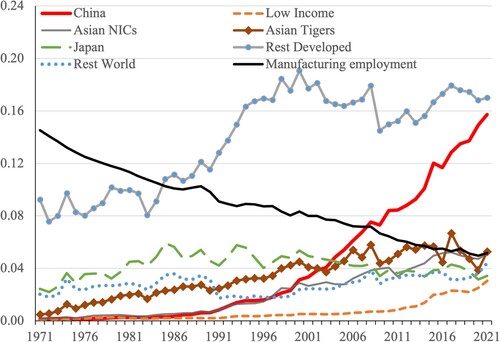
In many developed countries, including Australia, globalization prompted concerns that import-competing sectors and low-skilled workers faced lower employment and earnings. In Australia this was fuelled by the simultaneous rise in manufactured imports from China and shrinking Australian manufacturing employment. The share of imports from China in Australian consumption of manufactured goods increased from 0.6% to 15.7% between 1990 and 2021 (Figure 1), more than 30-fold in real US$ terms. At the same time, the share of the working-age population employed in manufacturing in Australia decreased from 9.8% to 5.2%.

Figure 1. Manufactured goods import penetration to Australia by country and manufacturing employment share of the working-age population.

Note and sources: Import penetration equals manufacturing imports divided by Australian manufactured good absorption (production plus imports minus exports). Imports are from the United Nations Comtrade database (https://comtrade.un.org/data/). Absorption is from the Australian Bureau of Statistics (ABS): Australian National Accounts: Input–Output Tables, cat. no. 5209.0.55.001 for 1989/90–2019/20. Missing yearly values from 1991 to 2012 are linearly interpolated. Other years’ estimated using growth rates (adjusted for trend difference) in national household consumption (ABS cat. no. 5206.0, tab. 3). Low income: as defined by the World Bank for 1989 excluding China (53 countries listed in Appendix A1 in the supplemental data online). Asian newly industrializing nations (NICs): Indonesia, Malaysia, the Philippines and Thailand. Asian Tigers: Hong Kong, Singapore, South Korea and Taiwan. Rest developed: all original Organisation for Economic Co-operation and Development (OECD) members except Japan and Australia. Rest of the world: all other countries covered by UN Comtrade data. Manufacturing employment of working age from 1984 to 2021 from ABS cat. no. 6291.0, tab. EQ12. Manufacturing employment of working age before 1984 from five-yearly censuses with other years interpolated. Working-age population from ABS cat. no. 3201.0, tab. 59.

The first main contribution of our study is to provide plausibly causal estimates of the effects of growth in manufacturing imports from China on local labour market (LLM) outcomes in Australia. We focus on employment in manufacturing from 1991 to 2006. This tracks the onset of the rise in Chinese imports to Australia until just before the Global Financial Crisis (GFC).² We divide Australia into 124 LLMs and construct local import exposure measures using employment and trade outcomes at the detailed level (55 manufacturing sectors).³

The 2010s has seen intensive study of the effect of growth in imports on labour market outcomes in developed countries. The most influential contribution has been by Autor et al. (2013), who examine the local effects of growth in imports from China for the United States. The study uses local variation in exposure to Chinese imports to identify causal effects. This large and unanticipated growth in imports from China following economic reform provides an ideal natural experiment for studying the effects of a rise in international trade (Autor et al., 2016).⁴

While we adopt the basic Autor et al. (2013) approach in providing new estimates for Australia, we also provide empirical support for the identification of causal estimates using recent developments on shift–share instrumental strategies (Adão et al., 2019; Borusyak et al., 2022; Goldsmith-Pinkham et al., 2020). Our study of Australia provides an interesting additional case study on the employment effects of increased imports from China. Australia is distinguished from other case studies, such as the United States, by its share of manufacturing in employment, its subsectoral structure and its labour market institutions.⁵ In addition, growth in Chinese imports occurred at the same time as Australia’s trade surplus with China grew via strong growth in mineral exports.

We find that for Australia an increase in an LLM’s exposure to Chinese imports by US$1000 per worker decreased the local share of the working-age population employed in manufacturing by 0.9 percentage points, on average. This is at the upper end of the range of effects across countries previously examined.⁶ The estimated effect is robust to a wide range of checks.

We also take the analysis a step further by asking: Why China? Australia also experienced increased imports from other developing Asian nations such as Singapore, South Korea, Indonesia and Thailand (Figure 1). We find that increases in imports from other Asian countries were not strongly related to the local manufacturing share in Australia in the period 1991–2006. This contrast with Chinese imports appears to be because Chinese imports tended to be in labour-intensive and slower growing industries.

Import-exposed locations experienced relatively higher rates of unemployment and lower labour force participation due to Chinese imports, despite some adjustment through regional labour mobility. There was no offsetting increase in local non-manufacturing employment. We also find higher part-time work and lower full-time employee income in more exposed labour markets.

The rest of the paper is organized as follows. Section 2 presents the empirical approach. Section 3 describes the data, the construction of our main variables and provides descriptive information. Section 4 reports the main empirical results for local manufacturing employment. Section 5 compares the effects and characteristics of imports from China with those from other countries in developing Asia. Section 6 discusses identification issues and describes robustness checks. Section 7 reports empirical results for other labour market outcomes: population mobility, employment in non-manufacturing industries, labour force participation, unemployment, part-time work prevalence and employee incomes. Section 8 discusses the results, including a comparative analysis with findings for other countries. Section 9 concludes.

2. METHODOLOGY

We estimate the local effect of Chinese imports on manufacturing employment in Australia following Autor et al. (2013). The main equation is: (1) $\mathrm{\Delta }{L}_{it}={\gamma }_t+{\beta }_1\mathrm{\Delta }IP{W}_{ait}+{\beta }_2{X}_{it}+{\epsilon }_{it}$(1) where $\mathrm{\Delta }{L}_{it}$ is the change in the share of the working-age population in LLM i employed in manufacturing between periods t and (t + 1); $\mathrm{\Delta }IP{W}_{ait}$ is the change in exposure in i to imports from China; ${\gamma }_t$ are time indicators; and $X_{it}$ is a vector of controls which may also affect local manufacturing employment changes.

The change in local exposure to imports from China is specified as: (2) $\mathrm{\Delta }IP{W}_{ait}=\sum _j(L_{ijt}/L_{it})(\mathrm{\Delta }{M}_{acjt}/L_{ajt})$(2) where $L_{ijt}/L_{it}$ is the share of employment in LLM i working in industry j at time t; $\mathrm{\Delta }{M}_{acjt}$ is the change in the value of imports to Australia from China in industry j between periods t and (t + 1); and $L_{ajt}$ is total Australian employment in industry j at time t. $\mathrm{\Delta }IP{W}_{ait}$ can be interpreted as the change in the value of Chinese imports per worker to an LLM, where increases in imports are apportioned to LLMs using initial local industry structure. The key coefficient of interest (${\beta }_1$) can be interpreted as the effect on the share of an LLM’s working-age population employed in manufacturing from a US$1000 per worker increase in local exposure to imports from China.

Variation in $\mathrm{\Delta }IP{W}_{ait}$ derives from two main sources: (1) differences between LLMs in the overall share of employment in manufacturing; and (2) uneven growth in Chinese imports across sectors within manufacturing combined with uneven sector-level employment across LLMs. Start-of-period manufacturing employment shares (source 1) explain one-third of the variation across LLMs. In our preferred specification of equation (1), we control for the local start-of-period manufacturing share. The focus is therefore on the effect of variation in exposure stemming from source 2.

Ordinary least squares (OLS) estimation of equation (1) may yield a biased estimate of the effect of $\mathrm{\Delta }IP{W}_{ait}$ on manufacturing employment. The main reasons for growth in imports from China to Australia are likely to have been productivity shocks which in turn lowered prices, plus the reintegration of China into the global economy. However, a further possible cause is increased demand by Australian consumers. In that case, imports to Australia from China would be positively correlated with industry demand shocks, imparting an upward bias to ${\beta }_1$. In addition, supply disruptions in Australia may both lower domestic employment and increase imports from China or elsewhere, imparting a downward bias.

To identify the effect of the supply-driven component of the increase in Chinese imports to Australia, $\mathrm{\Delta }IP{W}_{ait}$ is instrumented by $\mathrm{\Delta }IP{W}_{oit}$, constructed using changes in Chinese imports to eight other high-income countries: Denmark, Finland, Germany, Japan, New Zealand, Spain, Switzerland and the United States. Employment outcomes from period (t – 1) are used to mitigate potential simultaneity bias. (3) $\mathrm{\Delta }IP{W}_{oit}=\sum _j(L_{ijt-1}/L_{it-1})(\mathrm{\Delta }{M}_{ocjt}/L_{ajt-1})$(3) The motivation for this approach is that the rise in productivity in China caused increased import penetration to all high-income countries, and therefore using import flows from China to those other countries as an instrument should identify just the effect of increasing Chinese competitiveness. For this to hold, the increase in Chinese competitiveness must have created similar bundles of imports to other high-income countries as Australia, while the increase in imports to the other high-income countries must be uncorrelated with shocks to local labour demand in Australia.

We estimate equation (1) over three five-year intervals, 1991–96, 1996–2001 and 2001–06, as a stacked model. The start of the estimation period was chosen to coincide with the rise in Chinese imports to Australia. We end the period in 2006 because the instrument is likely to have its validity undermined after that time. The GFC caused correlated negative demand shocks across high-income countries that in turn contributed to a collapse in global trade, but Australia was largely immune from this reversal.

Our preferred model specification includes several variables that may affect local changes in manufacturing employment: (1) the initial share of employment in manufacturing; (2) the share of employment in routine occupations; and (3) an index measuring potential offshoring of occupations. The routine occupation share is intended to capture the effect of technological change (computerization and robotics) on labour demand. The offshorable potential of occupations captures an alternative dimension of globalization: the scope for locating tasks in different geographical locations. For (2), routine occupations are defined as those in the top third (1986 employment weighted) for routine task intensity (Autor & Dorn, 2013; Coelli & Borland, 2016). For (3), the index is taken from Firpo et al. (2011).

We follow previous research by including three additional covariates: (4) the share of the local population with a post-school qualification; (5) the local population share foreign-born; and (6) the local share of working-age females employed. Eriksson et al. (2019) find the resilience of regions to manufacturing shocks depends on local industries’ phase in the product cycle and on local education levels. Cadena and Kovak (2016) find greater mobility among immigrants than the native-born (especially low-skill workers) in response to adverse labour market shocks. Responses may also be a function of the labour force participation of females, historically less attached to the labour market (Gregory, 1991). We weight observations using each LLM’s share of the national working-age population. Robust standard errors (SEs) clustered by LLM are reported, along with SEs allowing for arbitrary correlations across industries (Adão et al., 2019; Borusyak et al., 2022).

3. DATA SOURCES, CLASSIFICATION OF LLMs AND DESCRIPTIVE STATISTICS

Employment data were obtained from the Australian Bureau of Statistics (ABS) for five-yearly Australian censuses conducted between 1986 and 2011. Import data were obtained from the United Nations (UN) Comtrade database at the Harmonized System (HS) six-digit level. Industries are classified at the three-digit level of the Australian and New Zealand Standard Industrial Classification (ANZSIC) 2006. Details of concordance of the employment and import data to ANZSIC 2006 over time are provided in Appendix A2 in the supplemental data online. All other covariates were constructed using information from the five-yearly censuses.⁷

Our import exposure measure is based on changes in Chinese imports within 55 three-digit manufacturing industries and three periods. We calculated an ‘effective’ sample size of 93.3 (inverse of the Herfindahl index: $HHI=1/\sum _{j,t}{s}_{jt}^2$) using industry-by-period employment shares, implying only modest concentration within manufacturing in Australia. The trade shocks relied upon in identification are real changes in Chinese imports to the eight instrument countries in US$1000 divided by lagged Australian industry employment. The mean trade shock is 167.4 with a standard deviation (SD) of 500.6 and an interquartile range of 140.4, providing considerable variation for identification. The intra-class correlations (ICCs) of the trade shocks within larger (15 two-digit) and more detailed three-digit industries are 0.090 (SE = 0.032) and 0.308 (SE = 0.052), respectively, implying modest within-two-digit industry correlation.

We construct LLMs for Australia in a manner consistent with US commuting zones (CZs), using commuting flows to create areas within which most individuals both live and work. Areas defined at the ABS’s Statistical Area 3 (SA3) level are aggregated to LLMs via the flowbca algorithm (Meekes & Hassink, 2018) using 2011 Census flows. This algorithm iteratively aggregates units based on flows between them. Each stage involves two units being merged into one, with the choice of which units to merge at each stage a function of flows between them. A stopping criterion determines when the process is terminated. Our application of this approach yielded 124 LLMs, with a minimum containment of 57%, a raw average containment of 89% and a weighted average (or population) containment of 95%. That is, for the 124 LLMs used in this study, 95% of workers in Australia live and work within the same LLM.⁸

For the 1991–2006 period, the share of imports from China in consumption of manufactured goods in Australia increased from 0.8% to 6.1% (Figure 1). The sectors where the largest increases in imports occurred were machinery and equipment and textile, leather, clothing and footwear (see Table A1 in the supplemental data online).

Changes in the exposure of LLMs to manufactured imports from China are described in Table 1 and Figure 2. Four features are evident. First, the increase in exposure is large, increasing by US$2874 per worker from 1991 to 2006 in the median LLM. Second, growth in exposure accelerated after China’s accession to the World Trade Organisation (WTO) in 2001. Third, there is high dispersion across LLMs in changes in exposure. Growth at the 90th percentile of the distribution is consistently four to six times higher than at the 10th percentile. Fourth, the largest increases occurred in metropolitan Victoria (VIC), South Australia (SA) and New South Wales (NSW), and in specific regional areas in VIC and NSW.

Figure 2. Changes in local exposure to Chinese imports per worker, 1991–2006.

Note and sources: See Table 1.

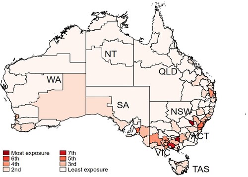
Table 1. Changes in local exposure to Chinese imports per worker (US$1000, 2006).

Percentile	1991–96	1996–2001	2001–06	1991–2006
10th	0.083	0.091	0.666	1.260
25th	0.183	0.171	0.978	2.060
50th	0.271	0.268	1.585	2.874
75th	0.406	0.430	2.303	4.025
90th	0.524	0.572	2.554	4.470

Sources: Authors’ calculations using equation (2). Employment data are provided by the ABS in customized tables. Trade data are from the UN Comtrade Database. Imports are deflated using the US personal consumption expenditure (PCE) deflator from FRED. See the text for details. LLMs (N = 124) are weighted by the initial share of the national working-age population.

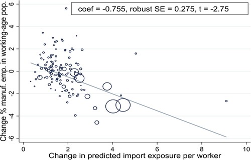
The correlation between growth in imports from China and local changes to manufacturing employment is illustrated in Figure 3. Predicted changes in local exposure⁹ are plotted against corresponding changes in the share of the working-age population employed in manufacturing. OLS estimation also reveals a significant inverse relation.¹⁰

Figure 3. Changes in local import exposure per worker and manufacturing employment, 1991–2006.

Note: Authors’ calculations, N = 124 local labour markets (LLMs). The estimated regression line controls for the initial share of employment in manufacturing and uses initial shares of the national working-age population as weights. Circle sizes represent the initial working-age population.

4. IMPACT ON MANUFACTURING EMPLOYMENT – MAIN RESULTS

Results from the main two-stage least squares (2SLS) analysis of the impact of Chinese imports on local manufacturing employment are reported in Table 2. Each model includes different sets of covariates. Model (1) only includes time indicators, model (2) adds the local start-of-period share of manufacturing employment, while model (3) also adds state fixed effects. Model (4) adds measures of the share of local jobs that are highly routine and the index reflecting the potential for occupations to be offshorable. Model (5) adds the three demographic covariates also included in previous studies. Model (6) includes the covariates recently recommended by Borusyak et al. (2022) for shift–share designs: using the five-year lagged share of manufacturing employment interacted with period indicators. Coefficient estimates on the instrumental variable, F-tests of the statistical significance of the instrument and the partial R² from the first-stage models are also reported.

Table 2. Relation between Chinese import exposure and local manufacturing employment, two-stage least squares (2SLS) estimates. Dependent variable: 5× annual change in the share of manufacturing employment in the working-age population (percentage points).

	(1)	(2)	(3)	(4)	(5)	(6)
Change in Chinese imports to Australia per worker (US$1000, 2006)	−1.131***	−0.980***	−0.907***	−0.860***	−0.831***	−0.925***
	(0.080)	(0.126)	(0.107)	(0.117)	(0.128)	(0.147) [0.130]
Percentage of employment in manufacturing^a		−0.028**	−0.057***	−0.066***	−0.059***	−0.060***
		(0.015)	(0.016)	(0.020)	(0.020)	(0.017)
Percentage of employment in routine occupations				0.057*	0.029	0.012
				(0.031)	(0.041)	(0.037)
Average offshorability index of occupations				−0.047	0.122	0.181
				(0.052)	(0.133)	(0.123)
Percentage of population with post-secondary education					−0.022	−0.034
					(0.027)	(0.025)
Percentage of population foreign-born					−0.012	−0.010
					(0.008)	(0.007)
Percentage of working age females employed					0.013	0.015
					(0.013)	(0.012)
Lagged % emp. in manuf. times year = 2001						0.021
						(0.018)
Lagged % emp. in manuf. times year = 2006						0.027
						(0.027)
State fixed effects	No	No	Yes	Yes	Yes	Yes
F-statistic	172.1	80.8	50.9	72.7	184.4	191.2
p-value	0.0000	0.0000	0.0000	0.0000	0.0000	0.0000
R^2	0.487	0.503	0.582	0.589	0.594	0.601
First-stage regression
Change in Chinese imports to other high-income countries per worker	0.0316***	0.0316***	0.0319***	0.0302***	0.0301***	0.0262***
	(0.0019)	(0.0026)	(0.0029)	(0.0041)	(0.0042)	(0.0058)
F-statistic	280.3	143.8	118.7	54.0	52.4	20.1
Partial R^2	0.923	0.888	0.881	0.833	0.829	0.691

Note: All regressions include period indicators. Standard errors clustered at the LLM level are provided in parentheses. Industry-clustered standard errors constructed using the Borusyak et al. (2022) method are given in brackets. Observations weighted by LLM’s initial share of the national working-age population. Number of observations is 372 (124 LLMs by three periods). *, ** and ***Statistical significance at 10%, 5% and 1% levels, respectively.

^a Lagged percentage of employment in manufacturing in column (6).

The estimated negative impact of increases in Chinese imports on the local share of employment in manufacturing is large and precisely estimated. In the model with all covariates in column (6), a US$1000 increase in Chinese imports per worker causes a 0.93 percentage point decrease in the local share of the working-age population employed in manufacturing (p < 0.001). The estimated impact decreases marginally as covariates are added but remains precisely estimated. For all models, the first-stage estimates show that the instrument is highly predictive.

In brackets in column (6), we also report the SE on import exposure using the industry-level regression method of Borusyak et al. (2022) that they call ‘exposure-robust’ and show is asymptotically equivalent to the SE proposed by Adão et al. (2019).¹¹ These SEs are valid under arbitrary cross-regional correlation in regression residuals due to common shocks at the industry level. The ‘exposure-robust’ SE clustered at the industry level is smaller than the LLM-clustered version. This contrasts with the findings of Adão et al. (2019) and Borusyak et al. (2022) when reanalysing the Autor et al. (2013) US study, where exposure-robust SEs tend to be 10–20% larger.

The large size of the estimated effect, together with the extent of variation between LLMs in growth in exposure, imply substantial dispersion in impacts across locations. For example, over the entire 1991–2006 sample period, an LLM at the 90th percentile in the distribution of increases in exposure has a predicted decrease in the manufacturing employment share of 2.8 percentage points; while an LLM at the 10th percentile has a predicted decrease of only 0.7 percentage points.

5 . CHINA OR DEVELOPING ASIA MORE GENERALLY?

While growth in Australian imports of manufactured goods from China since 1991 has been remarkable, imports from other Asian neighbours also grew strongly (Figure 1). Import penetration from the four Asian newly industrializing nations (NICs: Indonesia, Malaysia, the Philippines and Thailand) rose from 0.8% in 1991 to 3.2% in 2006, while from the Asian ‘Tigers’ (Hong Kong, Singapore, South Korea and Taiwan) import penetration rose from 2.5% to 5.4%. Import penetration from the large group of low-income countries (LICs)¹² has increased recently, but the rise from 1991 to 2006 was quite modest. We now investigate whether local exposure to increased imports from these Asian neighbours also led to reductions in local manufacturing employment over the 1991–2006 period. We construct import exposure measures using an appropriately modified version of equation (2) and again instrument using imports to our group of eight developed countries.

The results of 2SLS regressions including extra exposure measures are provided in Table 3. Adding exposure to the large group of LICs in column (1) changes the estimated effect of Chinese imports only slightly, but statistical significance is now lost. The coefficient on exposure to LIC imports is very large but is imprecisely estimated.¹³ In column (2) we add exposure to imports from the Asian NICs to the base model. The coefficient on Chinese import exposure becomes slightly more negative but is less precisely estimated. The coefficient on NIC import exposure is a noisy positive. Exposure to imports from China and the Asian NICs were quite highly correlated at the LLM level (correlation coefficient of 0.86), making it difficult to identify separate effects.

Table 3. Relation between Asian and low-income country (LIC) import exposure and manufacturing employment by LLM, two-stage least squares (2SLS) estimates. Dependent variable: 5× annual change in the share of manufacturing employment in the working-age population (percentage points). Explanatory variable: Change in imports from country/country group to Australia per worker (US$1000, 2006).

	Original exposure construction				Reduced industry detail
					Unadjusted	Adjusted for labour productivity
Import exposure	(1)	(2)	(3)	(4)	(5)	(6)
China	−0.991	−1.086***	−0.924***	−0.930***	−0.885***	−0.836***
	(0.756)	(0.288)	(0.147)	(0.158)	(0.159)	(0.164)
Other LICs	−67.13
	(449.9)
Asian NICs		1.415
		(1.583)
Asian Tigers			−0.143
			(0.445)
Asian NICs + Tigers				0.041	0.077	−0.816
				(0.358)	(0.241)	(1.279)
Absorption term						13.11
						(14.36)
F-statistic	33.6	138.3	186.9	180.3	172.1	193.9
p-value	0.0000	0.0000	0.0000	0.0000	0.0000	0.0000
R^2	0.591	0.581	0.594	0.602	0.588	0.605
First-stage F-statistics
China	40.2	20.8	17.7	20.1	144.9	123.0
Other country group	0.01	3.2	6.7	9.7	10.9	14.0

Note: All regressions include covariates from column (6) in Table 2. Standard errors clustered at LLM level are provided in parentheses. Observations are weighted by the initial share of the national working-age population. N = 372 for all regressions. *, ** and ***Statistical significance at 10%, 5% and 1% levels, respectively.

In column (3) we add exposure to imports from the Asian Tigers to the base model. In this case, the coefficient on Chinese import exposure remains negative and precisely estimated. The coefficient on Asian Tiger import exposure is a small noisily estimated negative. In column (4), we include combined import exposure from the Asian NICs and Tigers. The coefficient on Chinese exposure again remains a precisely estimated negative while exposure to imports from these other main Asian sources is unrelated to local changes in manufacturing employment.

What is specific about the manufactured product imports from China that explains why those imports led to reductions in manufacturing employment in Australia?¹⁴ To provide structure to our investigation of this question, we employ a simple deconstruction of industry-level employment as follows: (4) $L_{jt}={\displaystyle \frac{1}{{\alpha }_{jt}}D{P}_{jt}={\displaystyle \frac{1}{{\alpha }_{jt}}[A_{jt}-I_{jt}+E_{jt}]}}$(4) where $L_{jt}$ is employment in industry j at time t and $D{P}_{jt}$ is domestic (Australian) production of industry j output in period t. The term ${\alpha }_{jt}$ denotes domestic production per worker, reflecting Australian labour productivity in industry j in period t. Domestic production $D{P}_{jt}$ in turn equals absorption $A_{jt}$ in Australia of output of industry j in time t, minus imports $I_{jt}$ plus exports $E_{jt}$. This absorption is the ‘use’ of product within Australia as inputs into other industries and as final consumption by households and government.

From equation (4) we derive the following: (5) ${\displaystyle \frac{\mathrm{\Delta }{L}_j}{L_{j0}}={\displaystyle \frac{1}{{\alpha }_{j0}}\left[{\displaystyle \frac{\mathrm{\Delta }{A}_j}{L_{j0}}-{\displaystyle \frac{\mathrm{\Delta }{I}_j}{L_{j0}}+{\displaystyle \frac{\mathrm{\Delta }{E}_j}{L_{j0}}}}}\right]+\left({\displaystyle \frac{1}{{\alpha }_{j1}}-{\displaystyle \frac{1}{{\alpha }_{j0}}}}\right){\displaystyle \frac{D{P}_{j1}}{L_{j0}}}}}$(5) where $\mathrm{\Delta }$ indicates the change in the associated variable in industry j from period 0 to period 1, for example, $\mathrm{\Delta }{L}_j=L_{j1}-L_{jo}$ The proportional change in employment in industry j from period 0 to period 1 can be broken down into four components scaled by initial industry employment $L_{j0}$. The first three components are the change in absorption minus the change in imports plus the change in exports, all divided by initial labour productivity ${\alpha }_{j0}$. The final ‘residual’ term reflects changes in labour productivity over the period.

Based on equation (5), we explore three potential explanations as to why imports from China negatively affected Australian manufacturing employment while imports from other major Asian countries did not.

• Were Chinese imports more heavily weighted in industries where absorption $A_{jt}$ in Australia was growing more slowly? If so, these imports were more likely to replace domestic workers.

• Were Chinese imports predominantly in industries with low output per worker (${\alpha }_{j0}$)? If so, the same increase in import value would displace more local workers.

• Were imports from the Asian Tigers and NICs replacing imports from developed countries? Such imports would then be less likely to displace Australian workers.

Answers to these three questions can be observed in the correlation coefficients reported in Table 4 (for the scatter plots, see Figures A3–A5 in the supplemental data online). Import growth from the Asian Tigers and NICs are highly correlated with changes in Australian absorption over the 1991–2006 period. That is, import growth from these countries appears to be responding to increases in domestic consumption. Imports from China, on the other hand, increased across all industries, including those experiencing slow growth. Changes in imports from China are marginally more heavily weighted in low output per worker (high labour-intensive) industries. Changes in imports from the Asian Tigers and NICs, however, are much more heavily weighted in high output per worker industries. Finally, growth in imports from China are unrelated to import growth from developed countries, while imports from the Asian Tigers and NICs are positively related to such growth. Overall, there is little evidence that increased imports from either China or the Asian Tigers and NICs were simply replacing imports from developed countries. If anything, imports from the Tigers and NICs were adding to increased imports from developed countries, most likely in response to increased domestic absorption.

Table 4. Industry-level correlations with changes in imports from China and imports from the Asian Tigers and NICs, 1991–2006.

Change in imports per worker from:	China		Asian Tigers and NICs
Industries:	All	Excluding fuels	All	Excluding fuels
Change in Australian absorption	−0.09	0.01	0.96	0.57
Initial (1991) Australian production per worker	−0.15	−0.15	0.94	0.55
Change in imports per worker from developed countries	0.05	0.05	0.33	0.50

Note: Absorption and production data for Australia are from ABS input–output tables (see the note to Figure 1). Due to differences in industry detail provided in these tables, 55 ANZSIC three-digit manufacturing industries were combined into 34 consistent sectors in rows 1 and 2. Trade data are from UN Comtrade. Employment data are from the 1991 Census. All values are in 2006 real US$.

Imports from China thus appear to have had a more negative effect on Australian manufacturing employment for two reasons. Chinese imports have been more heavily weighted in industries experiencing slower growth in domestic absorption and that are more labour intensive.¹⁵ To ascertain whether these two features can explain our estimates at the LLM level, we re-estimate our model in column (4) of Table 3 after adjusting for both labour productivity and changes in absorption. These adjustments required the amalgamation of several manufacturing industries to match our information on industry-level absorption and output, reducing industry numbers from 55 to 34. In column (5), we present estimates equivalent to column (4), but after reducing the industry detail to 34. These estimates are very similar to those of column (4), providing comfort that the reduction in detail is not materially affecting our results. In column (6), we present estimates of our model adjusting for labour productivity and absorption. Specifically, we reconstructed the import exposure measures (both the endogenous and instrument versions) after dividing import changes by initial industry labour productivity (and multiplying by 100). We also added a control variable reflecting local changes in industry absorption, constructed akin to equation (2), but using changes in industry absorption divided by initial labour productivity rather than changes in imports.

To begin, the coefficient on productivity-adjusted Chinese import exposure is still negative and highly statistically significant. What is important here, however, is that the coefficient on adjusted imports from the Asian Tigers and NICs is now of essentially the same size as that on adjusted Chinese exposure, albeit not precisely estimated. This implies that after adjusting for labour productivity and absorption growth differences across industries, imports from both sources would have had comparable effects on local manufacturing employment. Also note the increase in model R², implying these adjustments added explanatory power.

6. IDENTIFICATION AND ROBUSTNESS

The estimation technique we employ uses a shift–share or Bartik (1991) instrument. We are combining local three-digit manufacturing sector shares with sector-level changes in Chinese imports to predict local exposure. Shift–share instruments have received considerable attention in recent literature, providing clarity regarding the underlying variation being used and the assumptions relied upon for identification. Goldsmith-Pinkham et al. (2020) argue that consistent estimation requires the local lagged detailed industry shares to be exogenous. Share exogeneity seems unlikely in our setting, as the prevailing local industry structure is almost certainly related to changes over time in the local manufacturing share of employment. Borusyak et al. (2022) argue that consistency can still be achieved if the industry-level changes in imports from China are numerous random shocks, even if local industry shares are not random. Our analysis relies on such an assumption.¹⁶

We discuss results of several robustness exercises recommended by Borusyak et al. (2022) in Appendix A3 (results are shown in Table A5) in the supplemental data online. A check on sensitivity to removing all five control variables or ‘confounders’ does result in a more negative coefficient estimate, but the change is not excessive. This modest effect suggests minimal potential bias, despite evidence of correlation between the import shocks and these ‘confounders’. Adding controls for each two-digit industry, which essentially allows for differential trends in outcomes within each of these sectors, led to the main coefficient becoming more negative.

The findings of other important robustness exercises are also discussed in Appendix A3 and presented in Table A6 in the supplemental data online. Our estimates are robust to: (1) measuring exposure with net imports, (2) estimation via a gravity model, (3) including the 2006–11 period, (4) controlling for changes in tariffs, (5) excluding remote areas, (6) measuring imports in Australian dollars, (7) changing the group of high-income countries used to construct the instrument and (8) excluding certain key industries.

Table A7 in the supplemental data online shows via a falsification test that future changes in imports from China do not affect past changes in the local share of the working-age population in manufacturing. Specifically, we regress changes in local manufacturing share from 1986 to 1991 on instrumented growth in Chinese imports over the 1991–2006 period plus the set of covariates from model (5) of Table 2. The coefficient on growth in Chinese imports was 0.027 (SE = 0.110). This provides further comfort that our estimates are causal effects and not simply capturing a trend decline in manufacturing in Australia.

7. OTHER IMPACTS

Differences in local exposure to Chinese imports imply heterogeneity in the magnitude of impact on local manufacturing employment. This may create an incentive for mobility. Workers displaced from manufacturing in one LLM may move to areas where job opportunities are better, or emerging industries in LLMs which have lost manufacturing jobs may attract new workers.

We find evidence of a negative impact of increases in imports from China on local working-age population (logged), as reported in Table 5. For all working-age, the predicted 1991–2006 growth in population is 10% lower in an LLM at the 90th percentile of increased exposure relative to one at the 10th percentile. To aid interpretation, working-age population growth over the period was around 20%.

Table 5. Population responses: relation between Chinese import exposure and the working-age population by LLM. Dependent variables: Change in log working-age population within each group. Explanatory variable: Change in imports from China to Australia per worker (US$1000, 2006).

Model	Sample	Coefficient	R^2	F-statistic	p-value
1	All	−0.0445***	0.549	33.5	0.0000
		(0.0084)
2	Bachelor’s degree or higher	−0.0222*	0.660	276.1	0.0000
		(0.0126)
3	Diploma or certificate	−0.112***	0.678	64.9	0.0000
		(0.0143)
4	No post-school qualification	−0.0223***	0.547	52.0	0.0000
		(0.0079)
5	15–34 years of age	−0.0507***	0.601	50.6	0.0000
		(0.0090)
6	35–49 years of age	−0.0150**	0.678	106.9	0.0000
		(0.0070)
7	50–64 years of age	−0.0649***	0.716	295.0	0.0000
		(0.0103)

Note: All regressions include covariates from column (6) in Table 2. Standard errors clustered at the industry level are provided in parentheses and constructed using equivalent industry-level regressions, as described by Borusyak et al. (2022). Observations are weighted by the initial share of the national working-age population. N = 372/165 for LLMs/industries, both by period. *, ** and ***Statistical significance at 10%, 5% and 1% levels, respectively.

Growth in Chinese import exposure is most strongly related to decreases in the local share of the working-age population with lower education levels, especially those whose highest qualification is a diploma or certificate. This may reflect differential mobility between LLMs but may also reflect fewer people acquiring those qualifications in exposed locations. The value of such qualifications likely fell as manufacturing employment decreased. Increased exposure is also related to larger relative declines in the local shares of the population aged 15–34 and 50–64.

We delve further into these population responses using 2006 Census data that records where people were residing five years prior. Increases in import exposure were largest during this subperiod of our sample. To understand more about the origins of the population responses we undertake two exercises: first, we decompose population change between LLMs into its component parts; and second, we compare labour market outcomes among those who changed LLM with those that did not.

Changes in LLM working-age populations can be decomposed into three main components: (1) internal migration flows from one LLM to another, (2) external migration flows from and to other countries and (3) the effect of initial local demographic structure. Demographic structure may add to (reduce) working-age population growth over a five-year period if the size of the cohort entering working age (aged 10–14 at the start of the period) is larger (smaller) than the size of the cohort exiting working age (aged 60–64). We provide details of this decomposition for 2001–06 in Table 6, both overall and broken down by quartile of predicted residual changes in Chinese import exposure.¹⁷

Table 6. Decomposition of LLM working-age population changes, 2001–06.

		Quantiles of predicted residual exposure
	Overall	Lowest	Second	Third	Highest
Internal inflows	9.08	16.51	8.80	3.66	14.36
Internal outflows	9.04	14.87	7.33	5.36	16.18
External inflows	6.80	3.91	7.22	8.75	4.34
External outflows plus residual	3.95	2.50	3.98	4.89	3.76
Demographic structure	4.31	4.52	4.35	3.95	5.46
Total population change	7.19	7.58	9.06	6.12	4.22

Note: All figures are percentages of the initial LLM working-age population. Quantiles of predicted residual exposure constructed from two-stage least squares (2SLS) regressions partialling out effects of control variables in column 6 of Table 2. External inflows and outflows also include flows from and to Australia’s external territories and migratory areas. External outflows plus residual constructed as a residual and includes effects of measurement error and local deaths.

Focusing first on the overall decomposition (first column in Table 6), internal migration is quite prevalent in Australia, with approximately 9% of the working-age population changing LLMs between 2001 and 2006. Inflows from overseas¹⁸ are also sizable (6.8%), while outward international migration plus residual¹⁹ was just under 4%. Demographic structure contributed a sizable 4.31% to overall working-age population growth of 7.19%.

Now looking at flows separately by import exposure quartile, internal outflows exceed inflows among the most exposed regions, implying internal migration may be responding to increased import exposure. External outflows plus residual are lower than inflows across all exposure groups, but the gap is smallest in the most exposed group. The contribution of demographic structure also differs across exposure groups with the largest contributions among the least and most exposed regions. If anything, demographic structure (having a ‘young’ population) may be partially offsetting the internal and external migration responses in the most exposed group.

Decompositions constructed separately for our three broad age groups (see Table A8 in the supplemental data online) reveal the following. (1) Mobility is highest among ages 15–34, but this mobility does not appear to be associated with increased Chinese import exposure. The negative relationship between increased exposure and population by LLM is driven by demographic structure for this age group. (2) Both internal and external mobility among ages 35–49 are associated with import exposure. The weaker relationship between exposure and population for this age group is due to offsetting demographic structure effects. (3) Internal and external mobility among ages 50–64 are closely associated with import exposure, with demographic structure partially offsetting this effect.

We now turn to comparing the labour market outcomes of internal migrants and individuals who remain in their LLM over the 2001–06 period. Labour force status and broad industry of employment shares are presented in Table 7, for all working age and by broad age group. Internal migrants (‘movers’ hereon) are less likely to be unemployed across all age groups. They are not more likely to be employed, however, with a higher share remaining out of the labour force (NILF). These employed and NILF shares differ considerably across age groups. Young movers are more likely to be employed and less likely to be NILF than stayers, while old movers are the opposite, likely reflecting moving for early retirement.

Table 7. Labour force status and industry of employment of internal migrants and stayers, 2001–06.

	All working ages		Ages 15–34		Ages 35–49		Ages 50–64
	Stay	Move	Stay	Move	Stay	Move	Stay	Move
Employed	72.83	72.32	70.49	75.61	81.57	83.38	65.57	50.32
Unemployed	3.18	2.09	4.63	2.67	2.66	1.60	2.00	1.41
NILF	23.98	25.59	24.89	21.73	15.78	15.02	32.43	48.27
Industry if employed
Agriculture	2.92	4.29	1.84	2.55	2.82	4.46	4.32	8.32
Mining	0.95	3.01	0.76	2.91	1.08	3.73	0.93	1.99
Manufacturing	11.46	9.16	10.50	8.54	12.42	10.31	11.32	8.95
EGWW	0.95	0.60	0.64	0.39	1.09	0.80	1.13	0.77
Construction	8.31	8.49	9.16	8.30	8.25	9.18	7.31	7.85
Services – high	34.34	30.25	28.89	26.75	36.59	32.81	38.12	34.95
Services – low	41.09	44.20	48.23	50.56	37.74	38.71	36.88	37.16

Note: All figures are percentages of each group. NILF, not in the labour force; EGWW, electricity, gas, water and waste; Services – high = information technology (IT), media and telecommunications; finance and insurance; rental, hiring and real estate; professional, scientific and technical services; education and training; health care and social assistance; arts and recreation; and Services – low = wholesale trade; retail trade; accommodation and food services; transport, postal and warehousing; administrative support services; public administration and safety; other services.

Movers are less likely to be employed in manufacturing across all age groups, which is understandable if moving was partly in response to reduced manufacturing employment possibilities. Movers are more likely to be employed in agriculture (particularly the old), mining and low skill services (particularly the young). Some workers may thus have moved for employment opportunities in traded sectors outside manufacturing. Employment in mining was expanding during 2001–06 as Australia’s mining boom began.

In summary, LLMs with higher import exposure have slower population growth due to smaller net internal and external flows in the population aged 35–64. The labour force status of internal migrants compared with non-migrants varies by age. Young non-employed movers are more likely to be unemployed while older movers are more likely to be out of the labour force. Employed movers are more likely to work outside manufacturing in the expanding mining and low-skill service sectors.

In locations where employment in manufacturing fell, adjustment may occur in ways other than population outflow: first, through offsetting increases in employment in non-manufacturing industries; and second, through higher unemployment and/or movement out of the labour force. Table 8 reports estimates of the impact of changes in import exposure on the shares of an LLM’s working-age population employed in manufacturing and non-manufacturing, who are unemployed, or who are out of the labour force.²⁰ Note that over the 1991–2006 period, the mean non-manufacturing share rose by 8.1 percentage points, the unemployment share fell by 4.5 percentage points and the share not in the labour force fell by 2.1 percentage points (see Table A2 in the supplemental data online).

Table 8. Relation between Chinese import exposure and labour force status by LLM, two-stage least squares (2SLS) estimates. Dependent variable: 5× annual change in shares of the working-age population by labour force status (percentage points). Explanatory variable: Change in imports from China to Australia per worker (US$1000, 2006).

Demographic group	Manufacturing employment	Non-manufacturing employment	Unemployment	Not in the labour force
All	−0.925***	−1.204***	1.149***	0.980***
	(0.130)	(0.352)	(0.192)	(0.186)
Bachelor’s degree or higher	−0.665***	0.840***	0.219***	−0.322**
	(0.205)	(0.245)	(0.078)	(0.141)
Diploma or certificate	−0.417**	−1.106***	1.130***	0.404**
	(0.209)	(0.373)	(0.172)	(0.175)
No post-school qualification	−0.992***	−1.650***	1.312***	1.325***
	(0.120)	(0.410)	(0.231)	(0.223)
Males	−1.227***	−1.260***	1.558***	0.949***
	(0.214)	(0.429)	(0.237)	(0.204)
Females	−0.630***	−1.072***	0.766***	0.934***
	(0.066)	(0.306)	(0.155)	(0.212)

Note: All regressions include covariates from column (6) in Table 2. Standard errors clustered at the industry level are provided in parentheses and constructed using equivalent industry-level regressions, as described by Borusyak et al. (2022). Observations weighted by the initial shares of the national working-age population. N = 372/165 for LLMs/industries, both by period. *, ** and ***Statistical significance at 10%, 5% and 1% levels, respectively.

In aggregate, the shares of the working-age population employed in manufacturing and non-manufacturing industries both decreased in response to an increase in Chinese imports. There is thus no offsetting increase in employment in non-manufacturing industries locally in response to declines in manufacturing.²¹ Adjustment occurs via higher unemployment and higher shares of the population who are out of the labour force. For example, a US$1000 increase in Chinese imports per worker causes a (relative) 1.15 percentage point increase in the share of the working-age population who are unemployed.

Table 8 also reports estimated impacts on groups of workers disaggregated by education and gender. The share of working-age males employed in manufacturing is more negatively affected by Chinese imports than for females, although both effects are precisely estimated (p < 0.001).²² There is a larger increase in unemployment among males than among females, in turn due to larger negative effects on employment in both manufacturing and non-manufacturing.

For those with a bachelor’s degree or above, increases in exposure had a smaller than average negative effect on manufacturing employment coupled with a sizable offsetting positive effect on non-manufacturing employment, resulting in modest growth in unemployment. By comparison, those whose highest education qualification was a diploma or certificate experienced both lower manufacturing and (although not significant) non-manufacturing employment. Hence, the increase in unemployment was much larger for this group. Among those with no post-secondary education, labour market outcomes were the most negatively affected. A large negative effect on manufacturing employment was compounded by a larger negative effect on non-manufacturing employment. Both unemployment and labour force exit were markedly higher for this group in affected locations.

A potential explanation for these patterns by education attainment is as follows. When manufacturing employment decreases, it is mainly low-skilled workers who become unemployed and remain living locally. Contemporaneously, other non-manufacturing industries are then drawn into the area. These industries are likely to employ workers with higher skill levels such as bachelor’s degree graduates.

In the first column of results in Table 9, we provide estimates of the effect of increased Chinese imports on the proportion of the employed working part-time.²³ We provide these estimates in aggregate and broken down by gender and education. In aggregate, the proportion of the employed working part-time rose in response to increases in Chinese import exposure at the local level. The effect was a little smaller for males than females and was quite modest among those with a post-secondary education qualification. The effect was large among those with no post-school education.²⁴

Table 9. Relation between Chinese import exposure, part-time work status and full-time employee income by LLM, two-stage least squares (2SLS) estimates. Explanatory variable: Change in imports from China to Australia per worker (US$1000, 2006).

		Full-time income
Population	Part-time employment	Persons	Males	Females
All	0.853***	−0.0077	−0.0130**	0.0027
	(0.321)	(0.0050)	(0.0064)	(0.0035)
Bachelor’s degree or higher	0.285	−0.0197**	−0.0333***	−0.0062
	(0.196)	(0.0083)	(0.0100)	(0.0068)
Diploma or certificate	0.330	−0.0254***	−0.0312***	−0.0258***
	(0.295)	(0.0064)	(0.0071)	(0.0069)
No post-school qualification	0.902**	−0.0007	0.0002	0.0019
	(0.381)	(0.0035)	(0.0045)	(0.0024)
Males	0.602**
	(0.300)
Females	0.974***
	(0.330)

Note: All regressions include covariates from column (6) in Table 2. Dependent variable in column 1 = change in the share of employed working part-time. Dependent variable in the final three columns = change in mean log real income of full-time employees (adjusted using Australian CPI). Standard errors clustered at the industry level are provided in parentheses and constructed using equivalent industry-level regressions, as described by Borusyak et al. (2022). Observations weighted by the initial shares of the national working-age population. N = 372/165 for LLMs/industries, both by period. *, ** and ***Statistical significance at 10%, 5% and 1% levels, respectively.

Real average income of full-time employees²⁵ (the cleanest proxy of wage rates available in the census data) was negatively related to increased exposure to Chinese imports, predominantly among males (last three columns of Table 9). The lack of response among those with no post-school education may be related to Australian wage-setting institutions which provide a floor for real wages.

8. DISCUSSION

How does the way LLMs in Australia adjusted to increased exposure to imports from China compare with adjustments in other countries? Table 10 summarizes results on patterns of adjustment for Australia and for four other countries for which evidence is available. To aid comparison, we report results for Australia using the original model specification of Autor et al. (2013): column (5) of Table 2. Some caution is necessary making these comparisons since the studies differ in approach. Nevertheless, several patterns emerge. First, an increase in exposure to imports from China caused a decrease in the local manufacturing share in all countries. The effect size is strongly related to the extent to which each country’s composition of manufacturing production by sector was correlated with the composition of growth in Chinese imports.²⁶ Second, non-manufacturing employment effects differ widely between countries. Australia is notable for its large negative effect – which in turn explains larger responses in unemployment and non-participation in Australia. Whereas Spain, where Chinese imports had the largest negative effect on the population share working in manufacturing, had substantial growth in non-manufacturing employment, sufficient to cause a decrease in unemployment. Donoso et al. (2015) attribute this growth to local construction booms. Third, adjustment in wages/income seem broadly similar between countries, with a smaller negative adjustment in Norway being the exception.

Table 10. International comparison of labour market impacts of a US$1000 (2006 US$) per worker increase in imports from China.

Country	Period interval	Share in manufacturing employment	Share in non-manufacturing employment	Share unemployed	Share not in the labour force	Wages/income, % change
Australia	5 years	−0.831	−1.129	1.030	0.923	−0.013
		(0.128)	(0.376)	(0.229)	(0.234)	(0.003)
United States	10 years	−0.596	−0.178	0.221	0.553	−0.008
		(0.099)	(0.137)	(0.058)	(0.150)	(0.003)
Germany	10 years	−0.113	−0.100	0.007		−0.0122
		(0.061)	(0.061)	(0.015)		(0.015)
			100 × log non-manufacturing employment	100 × log unemployed	100 × log not in the labour force
Norway	11 years	−0.079	0.262	0.907	0.071	−0.003
		(0.022)	(0.094)	(0.535)	(0.099)	(0.001)
Spain	4 years	−2.055	5.38	−13.77	1.80	−0.0123
		(0.441)	(2.27)	(11.36)	(2.71)	(0.0089)

Sources: Australia – impact on working-age population shares and log real income of full-time employees, 1991–2006: Tables 6 and 7.

United States – impact on population shares and log mean wage, 1990–2007: Autor et al. (2013, tabs 5–6).

Germany – impact on population shares and log median wages, 1988–2008: Dauth et al. (2014, tabs 3, 5). Estimated impact on manufacturing employment is for imports from China. Estimated impact for other outcomes is for imports from China and Eastern Europe. Euros converted into US$ using an exchange rate of 0.76.

Norway – impact on population share in manufacturing but for 100 × log population counts for non-manufacturing (private) employment, unemployed and not in the labour force, and log mean earnings (private sector), 1996–2007: Balsvik et al. (2015, tabs 3–5). Krone converted into US$ using an exchange rate of 5.7.

Spain – impact on population share in manufacturing but for 100 × log population counts for non-manufacturing (private) employment, unemployed and not in the labour force, and log mean wages, 1999–2007: Donoso et al. (2015, tabs 2, 8, 9, specification D).

Increased unemployment and exits from the labour force were higher in Australian locations exposed to increased Chinese imports. This may raise concerns regarding increased dispersion in labour market opportunities across the country. However, LLMs subject to increased exposure had marginally lower unemployment shares and clearly lower shares of population not in the labour force in 1991, prior to the rise of China (see Figure A7 in the supplemental data online). This suggests that such concerns should be tempered.

In contrast to Autor et al. (2013) for the United States, we find evidence of local population responses to increased exposure to Chinese imports in Australia. Both internal and external mobility in Australia is common, as observed in Table 6. For internal migration, approximately 9% of the working-age population changed LLMs over the 2001–06 period. This compares with 12.9% who changed CZs over the five years to 2000 in the United States (Molloy et al., 2011, tab. 1). Internal migration is thus no more prevalent in Australia than in the United States. In addition, labour market shocks more generally have been associated with inter-state migration responses in both countries: see Blanchard and Katz (1992) for the United States and Debelle and Vickery (1999) for Australia.

The different population responses in Australia and the United States are potentially due to differences in local responses in non-manufacturing employment. In Australia, local non-manufacturing employment also declined with increased exposure while this did not occur in the United States.²⁷ The ‘push’ from LLMs with deteriorating labour market conditions was thus likely stronger in Australia. The ‘pull’ from an expanding mining sector in more remote regions of Australia likely also contributed to mobility.

9. CONCLUSIONS

Massive growth in imports of manufactured goods from China to Australia occurred from the early 1990s onwards. This study examines the impact of that growth on LLM outcomes in Australia from 1991 to 2006. We find increased exposure to Chinese imports had a relatively large negative impact on the local share of the working-age population employed in manufacturing. The adjustment to this impact mainly came via increases in the shares of the population unemployed and out of the labour force.

The focus of this study has been manufacturing. This enabled straightforward comparisons with other developed countries experiencing similar growth in Chinese imports. For countries such as the United States, examining the impact of imports from China may be enough to tell the whole story of the consequences of trade with China. For Australia, which also experienced growth in its exports to China over the same period (particularly mining exports), that is unlikely to be the case. Therefore, in other work-in-progress we are exploring in more detail how the impact of increases in imports from China on employment may have been offset by higher levels of exports from Australia to China.

ACKNOWLEDGEMENTS

This paper is a substantially revised version of Maccarrone (2017). We received valuable comments from Philip McCalman, Gordon Hanson and the participants at two workshops at the University of Melbourne, the AASLE 2018 meetings in Seoul, ACE 2019 in Melbourne, ESAM 2021 and Queens University Belfast. We are grateful for the assistance received from the ABS in providing unpublished data used in the study.

DISCLOSURE STATEMENT

No potential conflict of interest was reported by the authors.

Additional information

Funding

This work was supported by an Australian Research Council (ARC) Discovery Grant [number DP160102269].

Notes

1. World trade has since declined to 44% of GDP in 2019. Source: World Bank indicators (https://data.worldbank.org/indicator/TG.VAL.TOTL.GD.ZS).

2. Declining employment in manufacturing has been of interest due to its impact on demand for workers by skill level (Charles et al., 2018a; Barany & Siegel, 2018) and because the uneven geographical distribution of manufacturing production within countries means that it can be associated with significant adjustment issues (Autor et al., 2020). Decreasing manufacturing employment has had consequences for social outcomes including health and marriage (Charles et al., 2018b; Autor et al., 2016, 2019).

3. Blanco et al. (2021) identifies the effect of Chinese imports on employment in Australia through industry-level differences in changes in import intensity. For an important study of the labour market impact in Australia of increased exposure to international trade, see Fahrer and Pease (1994).

4. The other main approach to identifying labour market effects of growth in international trade uses episodes of trade policy liberalization (Pierce & Schott, 2016; Dix-Carneiro & Kovak, 2017).

5. Manufacturing employment in Australia was in decline for two decades before 1990 but had remained steady in the United States over that period. The sectoral distribution of employment also differed. For example, food processing, relatively protected from trade with China, accounted for 18.4% of manufacturing employment in Australia, but only 8.1% in the United States. In contrast, trade-exposed electronic and computer equipment and electric machinery were 14.4% of manufacturing employment in the United States compared with just 6.1% in Australia.

6. The Autor et al. (2013) approach has been used to estimate the impact of growth in Chinese imports to Germany (Dauth et al., 2014), Norway (Balsvik et al., 2015) and Spain (Donoso et al., 2015).

7. The routine occupations and offshoring measures were constructed by linking the US DOT and O*NET information to the Australian occupation structure and using local occupation shares from census data. For variable summary statistics, see Tables A2 and A3 in the supplemental data online.

8. Our LLMs have containment measures close to those of US CZs: 62%, 88% and 93% for minimum, average and population containment, respectively (Fowler et al., 2018). For a more detailed discussion and analysis of local labour markets in Australia, see Meekes (2022).

9. These predictions are based on Chinese imports at the three-digit industry level to the set of eight developed countries we use as instruments.

10. For changes in manufacturing employment across regions, see Figure A1 in the supplemental data online.

11. The Borusyak et al. (2022) version is more straightforward to construct and better behaved in settings where industry shares are correlated across locations, as in our setting.

12. This LIC group comprises all countries (except China) defined as low income in 1989 by the World Bank. It includes several large Asian neighbours: India, Viet Nam, Sri Lanka, Pakistan and Bangladesh.

13. The first-stage model for LIC exposure is extremely weak, with a first-stage F-statistic of only 0.01. In addition, imports from China and these LICs are highly correlated.

14. For plots of relationships between import changes from China and from the Asian Tigers/NICs with employment changes at the sub-industry level, see Figure A2 in the supplemental data online.

15. Regarding the two remaining components of equation (5)(5) ${\displaystyle \frac{\mathrm{\Delta }{L}_j}{L_{j0}}={\displaystyle \frac{1}{{\alpha }_{j0}}\left[{\displaystyle \frac{\mathrm{\Delta }{A}_j}{L_{j0}}-{\displaystyle \frac{\mathrm{\Delta }{I}_j}{L_{j0}}+{\displaystyle \frac{\mathrm{\Delta }{E}_j}{L_{j0}}}}}\right]+\left({\displaystyle \frac{1}{{\alpha }_{j1}}-{\displaystyle \frac{1}{{\alpha }_{j0}}}}\right){\displaystyle \frac{D{P}_{j1}}{L_{j0}}}}}$(5) , changes in Australian manufactured good exports were uncorrelated with Chinese imports and positively correlated with imports from the Asian Tigers and NICs, likely reflecting increased global demand. The labour productivity ‘residual’ was only weakly related to imports from both sources.

16. We also constructed the Rotemberg weights as recommended by Goldsmith-Pinkham et al. (2020) (see Table A4 and Figure A6 in the supplemental data online for details). These ‘influence’ weights are closely correlated with the China import shocks (labelled ‘growth’ in Table A4 online), implying the shocks are driving our estimates. This keeps us comfortable with relying on the exogenous shock assumption.

17. Predicted residual exposure changes are the residuals from 2SLS regressions using predicted exposure from first-stage regressions as the dependent variable. These exposure measures thus have partialled out the effect of the control variables from column 6 of Table 2.

18. Including from external Australian territories and migratory areas.

19. International outflows are not observable at the LLM level in our data, so are constructed as a residual. This residual will also reflect measurement error (e.g., location five years ago is not recorded for approximately 12%) and local deaths. LLM-level deaths among the working age are also not observed, but across Australia the working age death rate from 2001 to 2006 was 0.34% (ABS release, cat. no. 3302.0 – Deaths, Australia, 2006).

20. For diagnostic statistics for these regressions, see Table A9 in the supplemental data online.

21. Table A10 in the supplemental data online provides estimates using alternative specifications. Although our negative estimate of the manufacturing share is robust to alternatives, the negative estimate on the non-manufacturing share is not. We are thus cautious in claiming that local exposure to Chinese imports necessarily also lowered non-manufacturing employment.

22. The more negative impact on males is likely explained by a larger share of males working in manufacturing than females. An equal proportionate decrease in employment causes a larger decrease in the share of males working in manufacturing.

23. For diagnostic statistics for these regressions, see Table A11 in the supplemental data online.

24. For estimates based on the original model specification of Autor et al. (2013), see Table A12 in the supplemental data online. These estimates are broadly consistent with those provided in Table 9.

25. The census income data are reported in 10–13 categories. We calculate average income within each LLM and demographic group using interval regressions.

26. The correlation between (1) the estimated effects on the manufacturing share (Table 10) and (2) the correlation between a country’s manufacturing employment shares and total exports from China from the period 1996–2007 (Balsvik et al., 2015, fig. 2) is –0.48.

27. Faber et al. (2020) found increased robot adoption in the United States led to internal mobility flows, which they attribute to non-manufacturing responses. The China import shock had little spillover onto non-manufacturing locally, whereas local robot adoption was associated with negative spillovers.

REFERENCES

- Adão, R., Kolesár, M., & Morales, E. (2019). Shift–share designs: Theory and inference. Quarterly Journal of Economics, 134(4), 1949–2010. https://doi.org/10.1093/qje/qjz025
- Anderson, K. (2020). Trade protectionism in Australia: Its growth and dismantling (Working Paper No. 2020/10). Arndt–Corden Department of Economics, Crawford School of Public Policy, Australian National University.
- Autor, D., & Dorn, D. (2013). The growth of low-skill service jobs and the polarization of the US labor market. American Economic Review, 103(5), 1553–1597. https://doi.org/10.1257/aer.103.5.1553
- Autor, D., Dorn, D., & Hanson, G. (2013). The China syndrome: Local labour market effects of import competition in the United States. American Economic Review, 103(6), 2121–2168. https://doi.org/10.1257/aer.103.6.2121
- Autor, D., Dorn, D., & Hanson, G. (2016). The China shock: Learning from labour market adjustment to large changes in trade. Annual Review of Economics, 8(1), 205–240. https://doi.org/10.1146/annurev-economics-080315-015041
- Autor, D., Dorn, D., & Hanson, G. (2019). When work disappears: Manufacturing decline and the falling marriage market value of young men. American Economic Review: Insights, 1(2), 161–178. https://doi.org/10.1257/aeri.20180010
- Autor, D., Dorn, D., Hanson, G., & Majlesi, K. (2020). Importing political polarization? The electoral consequences of rising trade exposure. American Economic Review, 110(10), 3139–3183. https://doi.org/10.1257/aer.20170011
- Balsvik, R., Jensen, S., & Salvanes, K. (2015). Made in China, sold in Norway: Local labor market effects of an import shock. Journal of Public Economics, 127, 137–144. https://doi.org/10.1016/j.jpubeco.2014.08.006
- Barany, Z., & Siegel, C. (2018). Job polarization and structural change. American Economic Journal: Macroeconomics, 10(1), 57–89. https://doi.org/10.1257/mac.20150258
- Bartik, T. J. (1991). Who benefits from state and local economic development policies? W. E. Upjohn Institute for Employment Research.
- Blanchard, O., & Katz, L. (1992). Regional evolutions. Brookings Papers on Economic Activity, 1(1992), 1–75. https://doi.org/10.2307/2534556
- Blanco, A., Borland, J., Coelli, M., & Maccarrone, J. (2021). The impact of growth in manufactured imports from China on employment in Australia. Economic Record, 97(317), 243–266. https://doi.org/10.1111/1475-4932.12604
- Borusyak, K., Hull, P., & Jaravel, X. (2022). Quasi-experimental shift–share research designs. Review of Economic Studies, 89(1), 181–213. https://doi.org/10.1093/restud/rdab030
- Cadena, B., & Kovak, B. (2016). Immigrants equilibrate local labor markets: Evidence from the Great Recession. American Economic Journal: Applied Economics, 8(1), 257–290. https://doi.org/10.1257/app.20140095
- Charles, K., Hurst, E., & Notowidigdo, M. (2018a). Housing booms, manufacturing decline and labor market outcomes. Economic Journal, 129(617), 209–248. https://doi.org/10.1111/ecoj.12598
- Charles, K., Hurst, E., & Schwartz, M. (2018b). The transformation of manufacturing and the decline in US employment. NBER Macroeconomics Annual, 33, 307–372. https://doi.org/10.1086/700896
- Coelli, M., & Borland, J. (2016). Job polarisation and earnings inequality in Australia. Economic Record, 92(296), 1–27. https://doi.org/10.1111/1475-4932.12225
- Dauth, W., Findeisen, S., & Suedekum, J. (2014). The rise of the East and the Far East: German labour markets and trade integration. Journal of the European Economic Association, 12(6), 1643–1675. https://doi.org/10.1111/jeea.12092
- Debelle, G., & Vickery, J. (1999). Labour market adjustment: Evidence on interstate labour mobility. Australian Economic Review, 32(3), 249–263. https://doi.org/10.1111/1467-8462.00112
- Dix-Carneiro, R., & Kovak, B. (2017). Trade liberalisation and regional dynamics. American Economic Review, 107(10), 2908–2946. https://doi.org/10.1257/aer.20161214
- Donoso, V., Martin, V., & Minondo, A. (2015). Do differences in the exposure to Chinese imports lead to differences in local labour market outcomes? An analysis for Spanish provinces. Regional Studies, 49(10), 1746–1764. https://doi.org/10.1080/00343404.2013.879982
- Eriksson, K., Russ, K., Shambaugh, J. C., & Xu, M. (2019). Trade shocks and the shifting landscape of U.S. manufacturing (Working Paper No. 25646). National Bureau of Economic Research (NBER).
- Faber, M., Sarto, A., & Tabellini, M. (2020). Local shocks and internal migration: The disparate effects of robots and Chinese imports in the U.S. (Working Paper No. 20-071; (revised 2022). Harvard Business School BGIE Unit. https://papers.ssrn.com/sol3/papers.cfm?abstract_id=3517458#.
- Fahrer, J., & Pease, A. (1994). International trade in the Australian labour market. In P. Lowe, & J. Dwyer (Eds.), International integration of the Australian economy (pp. 177–224). Reserve Bank of Australia.
- Firpo, S., Fortin, N., & Lemieux, T. (2011). Occupational tasks and changes in the wage structure (discussion Paper No. 5542). IZA. http://ftp.iza.org/dp5542.pdf.
- Fowler, C., Jensen, L., & Rhubart, D. (2018). Assessing US labor market delineations for containment, economic core, and wage correlation (draft). https://osf.io/ktx3h/.
- Goldsmith-Pinkham, P., Sorkin, I., & Swift, H. (2020). Bartik instruments: What, when, why, and how. American Economic Review, 110(8), 2586–2624. https://doi.org/10.1257/aer.20181047
- Gregory, R. (1991). Jobs and gender: A Lego approach to the Australian labour market. Economic Record, 67(Supplement), S20–S40.
- Levinson, D. (2018). US manufacturing in international perspective (R42135). Congressional Research Service.
- Maccarrone, J. (2017). The dragon Down Under: The effect of Chinese imports on Australian labour market outcomes (University of Melbourne, Honours Research Essay).
- Meekes, J. (2022). Agglomeration economies and the urban wage premium in Australia. Australian Journal of Labour Economics, 25(1), 25–53. https://ajle.org/index.php/ajle_home/article/view/8
- Meekes, J., & Hassink, W. (2018). Flowbca: A flow-based cluster algorithm in Stata. The Stata Journal, 18(3), 564–584. https://doi.org/10.1177/1536867X1801800305
- Molloy, R., Smith, C. L., & Wozniak, A. (2011). Internal migration in the United States. Journal of Economic Perspectives, 25(3), 173–196. https://doi.org/10.1257/jep.25.3.173
- Pierce, B., & Schott, P. (2016). The surprisingly swift decline of US manufacturing employment. American Economic Review, 106(7), 1632–1662. https://doi.org/10.1257/aer.20131578
- Pomfret, R. (2014). Reorientation of trade, investment and migration. In G. Withers, & S. Ville (Eds.), Cambridge handbook of Australian economic history (pp. 397–418). Cambridge University Press.