Internal migration dynamics of native and foreign workers: an impulse–response analysis of perturbation and resilience by means of a spatial vector autoregressive model

ABSTRACT

Why are certain labour markets more resilient to economic shocks? Why are some economies deeply affected by migration? Modern migration theory remains based on simplistic neo-classical utility maximizing assumptions, despite a failure to fully answer real-world migration questions. The aim of this paper is to show that neo-classical dynamics are differentiated between subpopulations that make up the workforce. Using disaggregated data from Germany and a dynamic spatial vector autoregressive model that allows for spillovers, the paper teases out several aspects of regional labour market resilience. Results highlight that regions stand to benefit from supporting place-specific policies tailored to local circumstances.

KEYWORDS:

• internal migration
• spatial resilience
• spatial model
• impulse–response
• population movements
• push and pull factors
• spatial vector autoregressive model

JEL:

• C32
• J15
• R12
• R23

1. INTRODUCTION

Migration remains an important research topic in the social sciences. The main questions that usually arise in internal migration studies are: Who is moving, why, and what are the economic consequences of this spatial redistribution of people? It is also important to understand whether the factors that cause people to move from one geographical area to another, and the spatial reorganization of people that arises from this, alter an area’s resilience to economic shocks. The answers depend on the characteristics of spatial labour markets, the differences in the relative socio-economic characteristics of places and populations, and the positioning of this in a geographical context (Kondoh, 2017). The totality of these factors can be viewed as a complex web of relations that is under constant perturbation from external economic shocks, generating a spatial equilibrium that adjusts dynamically and constantly over time. Consequently, a comprehensive and dynamic view on migration and spatial labour markets, which integrates the spatio-temporal disparities in the local characteristics and challenges faced by regions, may help explain why certain areas are more resilient to economic shocks and have an improved ability to adapt to new economic circumstances.

The growing literature on spatial resilience has focused on the relative vulnerability and resistance of different areas to similar economic impacts and highlighted that a more comprehensive and dynamic approach to labour market policy can explain and possibly help improve the adaptive capacity of regions and cities (Martin & Sunley, 2015; Wixe & Andersson, 2017). A starting notion to adopt such a view is that the neoclassical literature on migration lacks flexibility to describe the observed heterogeneity in migration outcomes.

The standard neoclassical literature that details the motivation for migration and its associated effects on both sending and receiving areas has paid particular attention to its relationship with labour dynamics. Labour migration, like other forms of migration, can essentially be understood as a simple mechanism for the improvement of an individual’s economic fortune. In this view, host regions may be seen as those that offer new employment chances and higher wages, while sending areas may be characterized by a downturn in economic opportunity. The difference in economic prospects provides opportunities to migrants to increase their welfare by making a geographical move (Nijkamp & Poot, 2015). A rise in the rates of employment in one area works as a pull factor, while a rise in the unemployment rate in another pushes people to leave. Inflows and outflows of workers then naturally rebalance employment rates by regulating the size of the workforce, thus acting as a force that counters spatial differentials in the characteristics of labour markets.

The early literature discussed migration behaviour on the basis of these economic principles (Harris & Todaro, 1970). It argued that a wage difference between a place of origin and destination combined with the likelihood of acquiring a job explains why certain people migrate and others stay. This neoclassical theory of migration also conjectures that labour migration itself may, in turn, have an impact on the labour market equilibrium (Massey et al., 1993). For example, several studies have focused on a two-way effect between migration and labour market variables, and have tried to find causality between the flow of migrants and labour market variables by applying either a structural model (e.g., Bilger et al., 1991; Carlino & Mills, 1987) or a time-series model (Lu, 2001; Partridge & Rickman, 2006).

It should be noted, however, that internal migration dynamics are not just the result of pure labour dynamics. In fact, it turns out that core labour market variables are often not sufficient to fully explain internal migration flows (Mitze & Reinkowski, 2011). Researchers have therefore extended the basic labour migration model by considering various factors including human capital endowment (Bröcker & Mitze, 2020), regional competitiveness factors (Clemens, 2016), housing prices (Peng & Tsai, 2019), population densities (Clemens, 2016) and environmental conditions (e.g., Napolitano & Bonasia, 2010). While extending the neoclassical theory of migration with additional variables has provided a rich framework with which to explain many dimensions of migration, it relies on an extrapolation of general principles across locations, populations and time. However, migration processes are complicated due to the heterogeneity of migrants and their different preferences (Luthra et al., 2016). In this paper we argue that further theory development could benefit from a more explicit treatment of differences in equilibrium dynamics at the level of subpopulations and a subsequent focus on the endogenous interaction between the flows of those subpopulations.

Concretely, internal mobility within a country consists of the movements of different subpopulations of migrants who may react differently to economic shocks, and whose migration may impact local economies in different ways. In turn, the movements of one group of people may trigger those of others. Different subpopulations may follow one another or compete for housing. This is highlighted in the literature on ‘crowding-out’ and exemplified by studies that show how different groups drive each other out through the housing market (Meen, 2016), or by recolouring the political orientation of areas (Jurjevich & Plane, 2012). This means that migration flows at the subpopulation level cannot be understood independently in the same way that regular flows within a network cannot be well understood in isolation (Chun, 2008; Chun & Griffith, 2011). Rather, one should expect disaggregated data on internal (domestic) migration in a country to reveal interactions between native and foreign migrants, and expect each group to be associated with different structural parameters.

Analysing the migration dynamics of different subpopulations jointly may thus yield better predictions of net migration responses and economic outcomes in light of economic shocks or labour policy interventions. If subgroups within an area react differently to a common economic shock, and if their flows subsequently trigger different spillover effects, then the composition of local populations is an important factor that determines the total system reaction to identical shocks. This makes demographic compositions an integral component of spatial resilience through its differentiating role in labour migration. In an attempt to shed new light on the dynamic aspects of migration and its role in economic outcomes, this paper studies the interactions between migration decisions of foreigners and native citizens, using German labour markets as a case study.

To this end, the paper studies a multivariate time series of migration flows in and out of 397 NUTS-3 regions in Germany throughout the period 2000–14. In particular, it studies the annual inflows and outflows of foreign residents and native citizens in the working age (18–64 years old), and relates them to annual changes in subnationally disaggregated macroeconomic variables. Since the data are characterized by dependencies between different variables across both space and time, the paper uses a spatial econometric model that is capable of parameterizing both types of dependencies. In particular, the spatio-temporal autocorrelation issues will be tackled by using a spatial vector autoregressive (Sp-VAR) model that allows for temporal autocorrelation, spatial dependence and interaction between spatial variables. The model is then used to study the effects of local perturbations in key economic variables by means of an impulse–response analysis. This produces interesting empirical results that confirm the hypothesized interactions and differences in the push and pull factors that drive flows of natives and foreigners.

The remainder of this paper is organized as follows. The next section discusses the background of internal migration in Germany. Section 3 presents our econometric model, while section 4 discusses the data used in our analysis. Section 5 then presents and discusses the results. Section 6 concludes.

2. MIGRATION BACKGROUND IN GERMANY

2.1. Migration after reunification

In recent years, the discussion on internal migration has clearly gained momentum in many European countries, including Germany. In the case of Germany, especially after its reunification, the conventional neoclassical theory of migration may well explain why and how the West received a large number of people from East Germany. Internal migration in Germany has been massively studied through the lens of East–West migration, and a large volume of studies was published after the reunification of Germany (Beck, 2011; Friedrich, 2008; Schneider, 2005; Schultz, 2009). It is generally found that, after the unification, East Germany not only experienced a rapid breakdown of its industrial complex, but also lost a large number of educated people, since skilled workers abandoned this region (e.g., Kontuly et al., 1997). In the aftermath of the reunification, in order to stop East to West flows of people, the government introduced several instruments, including funding to increase the standard of living through investment in housing (Michelsen & Weiß, 2010). This increased mobility within Eastern Germany.

Many studies document that most people who left East Germany were young and had an above-average education level (Heiland, 2004). Decressin (1994) studied migration flows between West German states and indicated that a wage increase in particular regions had a significant impact on the inflow of people from other regions, while a rise in the unemployment rate in a region relative to others reduced this flow. Furthermore, studies from the start of the millennium showed a strong relationship between local wages, unemployment rates and internal migration (e.g., Hunt, 2000; Parikh & Leuvensteijn, 2003). Burda and Hunt (2001) indicate that wage convergence between East and West from 1989 to 1992 played a significant role in the state-to-state migration patterns, while they found that changing unemployment was primarily a result, rather than a determinant, of East–West migration flows.¹

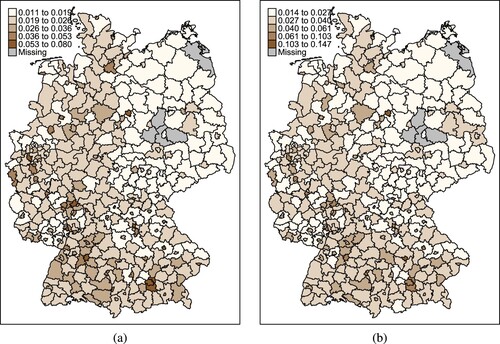
Today there remain East–West differences in the spatial distribution of economic variables, with notable shifts having occurred over time. Regional differences in terms of unemployment rate and gross domestic product (GDP) per capita are mapped in Figures 1 and 2. These are particularly well pronounced in the year 2000, with higher unemployment in the East. There appears to be continued convergence by 2014, with a new unemployment cluster in the West intensifying. The East–West divide is much less clearly pronounced in GDP per capita; this is mostly since the areas compare similarly with several high GDP clusters. However, it is clear that none of the major GDP centres is located in the East.

Figure 1. Unemployment rates in Germany in (a) 2000 and (b) 2014.

The spatial distribution of unemployment rates in the years 2000 and 2014 are mapped in these figures and showing the notable shifts having occurred over time. In the year 2000 unemployment rates are higher in East Germany than in West Germany. By the year 2014, there is visible convergence between both parts of the country. In the east, unemployment rates have fallen while there are unemployment hotspots emerging in the west.

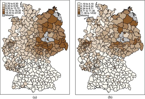
Figure 2. Gross domestic product (GDP) per capita (thousands) in Germany in (a) 2000 and (b) 2014.

The spatial distribution of GDP per capita for the years 2000 and 2014 are mapped in these figures. The East-West divide is much less clearly pronounced in GDP per capita than in unemployment rates, and predominantly highlight the major differences between urban cores and surrounding areas.

The relative level of homogeneity in migration flows, with clear common preferences across people united by shared motivations and opportunities to move, may contribute to the relatively good description that the simple neoclassical framework of migration has provided.

2.2. Migration after the millennium

In more recent times, migration flows have increasingly been driven by overall population dynamics. One reason is that Germany, in line with many other developed regions in the world, faces a growth in the number of older people (Börsch-Supan et al., 2014). In addition, there has been a negative growth rate in the overall population between 2002 and 2010 (Börsch-Supan et al., 2014). The combination of an ageing population and the decline in birth rates leads to an increase in the median age of the population and a falling share of younger people. This process drives a decline in cities’ labour supply across regions (Gløersen et al., 2016), and leads to changing demands for the types of goods and services that are locally produced. Shrinking local economies, in turn, reduce the degree to which those local areas are able to specialize in certain modes of production. This process may, in turn, affect job supply, and thus may become an important reason for specialized workers to move. The ageing process can, therefore, be expected to significantly impact the social structure and characteristics of different regions and cities in Germany. Changes in the characteristics of local livelihoods may in turn be an important factor for subsequent migration dynamics and may lead to changes in regional differentials in push and pull factors.

In part countering the age effects on labour markets and migration flows has been that following the Great Recession in 2008–09, Germany established its status as a top country for immigration within the European Union (EU) and has seen increasing numbers of refugees and economic migrants (Tanis, 2020). Questions about the integration of increasing numbers of immigrants into the labour market and society in general have taken centre stage in political discourse. It has also meant that the types of migration flows and the motivation for movement has shifted the nature of migration away from the East–West reunification lens that dominated early migration research in Germany. The recent trends in migration have instead made clearer that more recent migration flows are not homogeneous, but consist of the movements of many different types of people that may move for different reasons.

2.3. Migration and spatial labour market resilience

The differentiated nature of current migration dynamics in Germany introduces resilience-related questions. Since different areas face different types of migration flows under different local economic conditions, it is important to ask why certain labour markets are resilient to shocks while others grapple with self-reinforcing declines in fortunes. Resilience can be viewed as the capacity of a system to resist perturbations and to return efficiently to equilibrium after a disturbance. Spatial resilience focuses specifically on the place-specific consequences of shocks, and focuses on the ability of local socio-economic systems in different areas to bounce back to desired functions after unexpected shocks occur (Brunetta & Caldarice, 2020). In this way, it provides a framework to integrate analyses of resistance, adaptation and transformation of areas into local policies. There are many aspects to resilience, many related to one another (see Pascariu et al., 2022, for a systematic review of a large number of studies). In the current paper, we are particularly interested in understanding how similar local economic shocks lead to different labour migration outcomes, focusing on the narrow role that different migration dynamics of subpopulation play in shaping differentiated outcomes. This may help contribute to the overall understanding of why certain areas are more successful in retaining the local workforce than others, while in other areas abandonment and economic decline reinforce each other leading to vastly different outcomes over the long run.

Our integral analysis focuses on flows of native and foreign residents in Germany and will seek to test the proposition that the composition across these two subpopulations, that differ inherently in terms of socio-economic status, cultural preferences, and particularly income, is a critical determinant of local migration flows. The analysis proceeds in the understanding that the behaviour of these population groups is different, that the coming and going of different people may be associated with different economic consequences, and that spatially dependent factors among neighbouring areas are co-determining the regional flows. The analysis will explore how in this setting, local shocks lead to spatially differentiated effects, thereby producing a spatial resilience effect that shapes the total outcome of comparable local shocks. Importantly, if subgroups within an area react differently to a common economic shock, and if their flows subsequently produce different economic spillover effects, then the composition of local populations is an important factor that determines the total reaction of the labour force to what initially seem identical shocks.

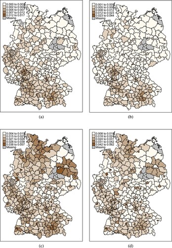
Figure 3 shows that native Germans and foreigners concentrate in different areas, while both are clustering spatially. The clusters largely suggest that both population groups cluster near similar populations, and away from populations in the opposing groups. An East–West gradient is not immediately clear in the population compositions. It is thus interesting to analyse how the different migration flows interact with each other in the changing economic environment. To disentangle migration into the multiple dynamics described, our study applies a time-series vector autoregressive (VAR) model with a spatial autoregressive specification. In this way, we allow for causality to run not only between labour market variables and migration flows, but also between the inflows and outflows of migration.²

Figure 3. Inflow of internal migrants (aged 18–64) in Germany as a share of the total population in each county: (a, b) the foreign working population; (c, d) the German working population; (a, c) 2000; and (b, d) 2014.

Inflow of internal migrants (between 18-64 years old) in Germany as share of total population in each county. This figure shows that native Germans and Foreigners concentrate in different areas, while both groups are clustering spatially.

3. DATA AND DESCRIPTIVE STATISTICS

The main part of the dataset is constructed from internal migration statistics from the Federal Statistical Office of Germany. Specifically, it consists of information on the annual number of individuals moving from one Kreis (the English word is county) in Germany to another for every pair of counties during the period 2000–14.³ Furthermore, the total number of movers is available by sex, age groups (≤ 18, 19–25, 26–30, 31–50, 51–65 and ≥ 66 years), and a nationality indicator, which distinguishes between Germans and non-Germans.⁴ The data do not include migrants who are foreign-born and move into the country. Importantly migration flows concern individuals who changed their residential place, therefore the data do not relate to commuting. In this study we focus on the working-age population (18–64 years) of both Germans and foreign residents, as this group has a higher mobility for different reasons (e.g., employment, family, etc.). The resulting net flows are summarized in Table 1.

Table 1. Descriptive statistics of the main variables (mean values for each year).

Year	Internal migration of Germans	Internal migration of foreigners	Gross wage (€)	Unemployment rate (%)	Gross domestic product (GDP) per capita(€)
2000	4399	728	€23,776.79	9.39%	€24,078.74
2001	4431	786	€24,280.62	9.25%	€24,658.96
2002	4412	795	€24,590.10	9.91%	€24,955.95
2003	4415	767	€24,863.39	10.71%	€25,066.79
2004	4385	729	€24,999.73	10.74%	€25,691.98
2005	4362	669	€25,043.26	12.14%	€26,082.25
2006	4366	643	€25,230.52	11.09%	€27,192.16
2007	4441	645	€25,622.50	9.16%	€28,513.83
2008	4555	664	€26,164.65	7.77%	€29,148.90
2009	4545	676	€26,004.53	8.49%	€28,054.51
2010	4498	684	€26,706.18	7.74%	€29,616.27
2011	4725	749	€27,569.77	6.97%	€31,607.74
2012	4619	838	€28,321.32	6.75%	€32,149.36
2013	4631	994	€28,933.05	6.83%	€32,721.81
2014	4573	1236	€25,868.67	5.91%	€33,070.31

Note: Descriptive statistics are calculated by aggregating district-level figures to a country total by sum (internal migration of Germans and foreigners thus represent the total number of that particular subpopulation who moved in a given year) or arithmetic mean (gross wage, unemployment rates and GDP per capita), thus giving each district equal weight. Internal inflows and outflows sum identically when the balance of flows is zero, which holds, by definition, for internal flows at the country level and thus approximately here, as only five districts have been excluded. Gross wages and GDP per capita are expressed in euros, unemployment rates in percentage points.

The counties for which the migration statistics are recorded are initially year-specific, that is, they correspond to the delineation of the current year. To ensure compatibility, consistent counties are constructed that follow the 2013 delineation. In most cases this can be easily done because boundaries have not changed. In some cases where boundaries did change, flows can be reproduced with the existing information.⁵ For five counties it is not possible to construct delineations that are constant over time.⁶ These counties are dropped from the sample, meaning that migration flows into and out of those counties are not included in the empirical analysis. This leaves a total of 397 counties and a total of 1,893,992 between-counties migration flows (each origin–destination pair had a positive flow at the annual level). The between flows are summarized at the county level, and the study focuses on total annual in- and outflows at the NUTS-3 administrative level. This reduces dimensionality of the data and simplifies the analysis by avoiding issues related to sparse and zero-flow data that often need treatment in origin–destination models. This simplification allows us in turn to expand the model dimension on other fronts by linking changes in total in- and outflows to changes in various local economic variables. Rather than suggesting that causality moves from the flows on one origin–destination pair onto the flows on another origin–destination pair, our analysis focuses on the interactions between changes in total in- and outflows of an area, and on subsequent interactions with the economic outcomes of that area. We will in turn also allow the local area changes in all variables to interact spatially with those in surrounding regions.

As can be observed from Table 1, the internal migration flow data are supplemented by a number of important regional characteristics. To model the functional relationships with changing economic conditions, we use data on annual GDP per capita and annual disposable income per capita at the county level (both provided by the Federal Statistical Office) and the regional unemployment rate (provided by the Federal Employment Agency).⁷

The three measures of economic conditions appear to display considerable cyclical fluctuations. Disposable income per capita and GDP per capita grew over time, with the exception of a temporary drop during the Great Recession. The average county-specific unemployment rate increased between 2001 and 2005, reaching a peak of more than 12%. This coincided with clear lower total movement in the subsequent period 2004–06. Over the following years, the average unemployment rate fell to below 6%, coinciding with increased total movement in 2010–14. The decline in the unemployment rate after 2006 is related to the labour market reforms which came into force between 2003 and 2005. A fundamental change in this reform, among other labour market changes, was the abolition of means-tested unemployment benefits that an unemployed person could receive up till retirement age (Schneider et al., 2019). The average county-to-county migration flow of German nationals stands at more than 4000 persons each year and is considerably larger than the average migration flow of foreigners, which only exceeded 1000 in 2014. By contrast, the variation in the size of the average migration flows is considerably smaller for German nationals than for foreigners. While the average flow of German nationals was about 4% larger in 2014 than in the year 2000, the corresponding increase for foreign migration flows is almost 70%. Increases in internal migration flows of foreigners are particularly pronounced from 2011 onward, whereas there is no corresponding development for Germans. Moreover, there is evidence that foreign internal migration flows contracted more than the migration flows of German nationals during the period 2003–05 when unemployment was relatively high and increasing.

4. A SPATIAL ECONOMETRIC VAR MODEL WITH A STOCHASTIC IMPULSE–RESPONSE STRUCTURE

4.1. Specification

Weidlich and Haag (1988) propose a conceptual dynamic migration model that is built up from the micro-level to the higher organization level of say a country. They discuss an example of native Germans and guest workers, close to our analysis, and that a population consists of different subpopulations that each have different migration behaviour and follow different migration dynamics. They subsequently explain that a migration theory defined for a single population (explicitly or implicitly assumed to be homogeneous) in practice only accounts for an average migratory behaviour of many possible existing subpopulations. We emphasize here that the shortcomings of such simplified theories run deeper. The migration patterns of different subgroups may interact with each other, for instance, in a mutually reinforcing way, leading to different average outcomes for every mixture of those subgroups. Moreover, if the migration flows of these different subgroups trigger different economic outcomes, and react differently to economic perturbations, then this average outcome may hide a high degree of heterogeneity. The idea of the model proposed here is to model migration at the subpopulation level dynamically, thus allowing the subpopulations to make individual reference to different economic variables, to one another, and to the values in nearby regions.

The backbone of the model adopted here follows a time-series VAR structure that allows the direction of causality to be investigated by using the arrow of time (Sims, 1972).⁸ The VAR has traditionally been applied in the context of multiple time series, but can also be applied in a panel setting, in which case it is often referred to as a panel VAR. The panel VAR assumes that areas are independent of one another but follow similar interactions based on shared parameters, which arguably only makes sense in a non-spatial or limited spillover context where cross-sectional observations are made in homogeneous groups (e.g., Wang et al. (2022)).

Borjas et al. (1997), Schoeni (1997) and LeSage and Fischer (2010) discuss methodological problems by studying migration dynamics related to spatial and temporal correlations in spatial panel data. They use a panel time series and assume that spatial residuals are independent after differencing over the time dimension and controlling for important variables. In the present analysis, the panel VAR is extended by a spatial autoregressive component that accounts for contemporaneous spatial spillover dynamics. This extension explicitly allows spatial dependencies to exist after differencing the data. The spatial autocorrelation component controls for possible neighbourhood spillover mechanisms that can be expected to occur as an equilibrium result of the German labour market network (Anselin & Griffith, 1988). The model is referred to as a spatial VAR (Sp-VAR). The literature on Sp-VAR modelling is still fairly new; spatial panel methods are discussed by Elhorst (2010). Stochastic properties of the spatial vector moving average (Sp-VAR) and estimation are discussed by Beenstock and Felsenstein (2019) and Andrée (2020).⁹

The combination of the VAR structure with a spatial autoregressive component is rather novel; it essentially treats all variables as dependent variables in a system of equations in which each equation represents a spatial econometric time-series model. The system thus allows for spatial spillovers within each subprocess while also allowing for interactions between the subprocesses, each interaction effect subsequently leading to new spatial spillover effects. This provides a flexible and coherent picture of the joint processes from which we can infer the direction of relationships while controlling for region-wide impacts that are a consequence of changes that are initially local.

In our study, we employ a parsimonious Sp-VAR specification in which the cross-sectional dimension is indexed by $i=1,\dots ,N$ and the time dimension is indexed as $t=1,\dots ,T$. In other words, internal migration in Germany is observed at discrete time intervals over a set of $N$ spatial units. Let $y_{\mathrm{i}\mathrm{k}\mathrm{t}}$ take the value of the $k$-th random variable $\left(k=1,2,..,K\right)$ registered on the $it$-th location in the space–time dimension, and stacking observations by location into $K$ vectors $Y_{tk}$, our Sp-VAR with $p$ lags and $K$ cross-sectional time-series variables is specified as the following system of equations: (1) $\begin{array}{cc}\mathrm{\Delta }{Y}_{1,t}& ={\alpha }_{1,g}+{\rho }_{1}W\mathrm{\Delta }{Y}_{1,t}+\sum _{p=1}^P\sum _{k=1}^K\left({\text{β}}_{1,pk}\mathrm{\Delta }{Y}_{k,t-p}\right)+{\tau }_{1}t+{ϵ}_{1,t}\\ \mathrm{\Delta }{Y}_{2,t}& ={\alpha }_{2,g}+{\rho }_{2}W\mathrm{\Delta }{Y}_{2,t}+\sum _{p=1}^P\sum _{k=1}^K\left({\text{β}}_{2,pk}\mathrm{\Delta }{Y}_{k,t-p}\right)+{\tau }_{2}t+{ϵ}_{2,t}\\ ⋮& =⋮\\ \mathrm{\Delta }{Y}_{K,t}& ={\alpha }_{K,g}+{\rho }_{K}W\mathrm{\Delta }{Y}_{3,t}+\sum _{p=1}^P\sum _{k=1}^K\left({\text{β}}_{K,pk}\mathrm{\Delta }{Y}_{k,t-p}\right)+{\tau }_{K}t+{ϵ}_{K,t}\\ & & \end{array}$(1)

where ${\alpha }_{k,g}$ is an East/West-specific constant in the $k$-th equation; ${\rho }_k$ is a scalar parameter that controls the strength of spatial autocorrelation in the $k$-th cross-sectional time series; $W$ is an $N\times N$ contiguity matrix which is similarly defined for each equation; ${\text{β}}_{k,pk}$ is an autoregressive parameter in equation $k$ for each combination of lags and variables $pk,\dots ,PK$; the scalar parameter ${\tau }_k$ allows for a linear trend; and ${ϵ}_{K,t}$ is a vector of $N$ residuals at time $t$ for variable $k$. The residuals are assumed to follow a Student’s t distribution with parameters ${\sigma }_k$ (variance) and ${\lambda }_k$ (degrees of freedom). Finally, $\mathrm{\Delta }$ is used to indicate that we work with first-differenced series.¹⁰ Our spatial autoregressive vector consists of a connectivity matrix; an $N\times N$ matrix $W$ with weights $w_{ij}$ specified a priori such that $w_{ij}$ and $\sum _{j=1}^N{W}_{ij}=1$. This matrix reflects the network of relationships in the system. Our weights matrix is based on a standard first-order contiguity scheme, which reflects the existence of a common border between each two counties in order to capture the spatial effect of internal migration from one county.¹¹ The average number of neighbours is eight, and ranges from one to 17.

The system is estimated using maximum likelihood; the estimator for the case of $t$-distributed residuals was developed by Andrée (2020). Note that the $t$-distribution allows for more kurtosis while it can also allow residuals to follow a Normal distribution (by setting $\lambda \to \mathrm{\infty }$). When $\lambda$ is small, the distribution allows for fat tails to capture non-Gaussian features of the data that may, for instance, result from unmodeled heterogeneity.¹² In this case, the estimator behaves more like the 50th percentile estimate and provides some robustness in the presence of outlier data. Since the time series are relatively short, the model is estimated using $p=1$. To find a parsimonious but appropriate stochastic representation of the historical data, the model is estimated using step-wise Akaike information criterion (AICc) shrinkage following the literature on model selection (Granger et al., 1995). Note that this also works well in the case of model misspecification (Sin & White, 1996), in which case the results are to be understood as pseudo-true, meaning that it is the closest stochastic representation of the correct causal structure out of all models generated under the full parameter space (Andrée, 2019, 2022).

Even though equations (1) are fully parametric and transparent econometric equations whose parameters and confidence intervals could be interpreted in the usual way, the high number of parameters and the interactions between many variables make it difficult to understand the net effect of a change in values in one of the variables. In particular, an initial change in one variable may set in motion a causal chain of reactions that undo or amplify an initial shock over the course of a certain time interval. Some basic interactions would however be represented directly by individual parameter values. For instance, (1) if increasing unemployment slows/accelerates a subsequent migration flow, we would expect a negative/positive parameter; (2) if economic growth slows/accelerates a subsequent migration flow, we would expect a negative/positive parameter; and (3) if wage growth slows/accelerates a subsequent migration flow, we would expect a negative/positive parameter.

The model can capture crowding-out effects, but these depend on the net balance of flow changes and thus a combination of the parameters that regulate individual in- and outflows. The impact of migration flows on economic outcomes similarly involves multiple parameters. To understand such combined effects of all interactions in this complex system, equations (1) are used for an impulse–response analysis, simulating from parameters drawn from their estimated distributions. The main purpose of the analysis is to describe the evolution of all the model’s variables in reaction to an initial (local) shock in one of the variables.¹³

A caveat of the model laid out in equations (1) and the simulated impulse–response analysis is that it does not assess contemporaneous reactions between variables. The only contemporaneous effects in the model are the spatial spillovers; all other interactions are to be understood as Granger-causal, in the sense that all effects in the model concern sequential time-series interactions.¹⁴ The results thus provide a coherent picture of migration dynamics over the time dimension, while neighbouring economic or migration dynamics may influence each other simultaneously. Intuitively, such a view on migration is reasonable: contemporaneously, migration decisions and economic spillovers may depend on neighbouring conditions, captured by the spatial interaction components, as economic agents may rapidly inform one another through price action in local markets and social channels. The assimilation of macroeconomic impacts from one economic variable into another or from economic variables onto migration decisions, captured by the VAR structure, does not happen instantaneously and may occur over the time dimension.

It is also important to note that the simple neighbour-based spatial structure imposes a degree of smoothness on the type of spillovers allowed in the model that leads to possible limitations that become particularly relevant in the context of forecasting. The direct neighbour spillovers are more appropriate for the economic variables, but for migration flows they describe only one component of spatial dependence. For more accurate forecasting results, direct connections between more distant areas may also need to be captured, possibly by allowing for different dependence parameters. Such direct relationships are likely present in the data, for instance, because there are agglomerated industries that are distant in space but compete for similar workers. In the current setting where the focus is on inference, the specification of the spatial weights matrix has intentionally been kept simple in order to help summarize migration spillovers at a level that is easy to comprehend.¹⁵ Nevertheless, the contiguity matrices should capture economically meaningful dynamics. For instance, it is highly likely that growth and changes in wages and unemployment rates spill over to neighbouring regions. This would be captured by positive values in the spatial dependence parameters. Migration flows may similarly feature spatial dependence, for instance because neighbouring areas may share common push and pull factors and because neighbouring flows may accelerate each other. Again, such reinforcing dynamics would be captured by positive spatial dependence parameters. As we shall show in the application, it is also possible to use the model to trace the net impact of a change in one area onto its direct or higher order neighbours.

5. RESULTS AND DISCUSSION

5.1. Parameter estimates

Table 2 presents the estimation results for our Sp-VAR model (AICc), as described above. We note that the blank spots are parameters that have been set to zero in order to minimize the AICc.

Table 2. Spatial vector autoregression results.

	GDP per capita	Unemployment rate	Gross wage	German		Foreign
				Inflow	Outflow	Inflow	Outflow
L.German inflow	−0.029**	−0.032		−0.262***		0.153***	−0.062
	(0.009)	(0.021)		(0.014)		(0.037)	(0.038)
L.German outflow		−0.078	0.016		−0.221	−0.117
		(0.024)	(0.004)		(0.013)	(0.043)
L.Foreign inflow	−0.009**	0.013		0.009*	−0.030***	−0.141***	0.191***
	(0.003)	(0.007)		(0.004)	(0.003)	(0.013)	(0.012)
L.Foreign outflow	−0.007*	0.015*	−0.002			0.065***	−0.223***
	(0.003)	(0.007)	(0.001)			(0.015)	(0.014)
L.Unemployment	0.010*	−0.052***	−0.003	−0.045***	−0.013**	0.027	0.020
	(0.004)	(0.010)	(0.002)	(0.006)	(0.097)	(0.016)	(0.364)
L.GDP	−0.021	−0.224	0.020	0.112	0.038		0.146
	(0.014)	(0.031)	(0.006)	(0.018)	(0.016)		(0.046)
L.Wage	−0.064*	0.308***	−0.055***			0.882***	0.529***
	–(0.029)	(0.068)	(0.013)			(0.117)	(0.102)
Rho	0.570***	0.767***	0.899***	0.236***	0.319***	0.311***	0.166***
	(0.015)	(0.010)	(0.007)	(0.021)	(0.020)	(0.024)	(0.020)
Constant	0.719***	2.097***	0.177***	−0.877***	1.374***	−10.176**	−5.325***
	(0.111)	(0.258)	(0.047)	(0.161)	(0.097)	(0.872)	(0.364)
East	0.389**	−2.888***	0.269***	−0.521**	−3.114***		−1.482**
	(0.121)	(0.271)	(0.051)	(0.172)	(0.148)		(0.479)
Trend	0.063***	−0.348***	−0.012*	0.082***	−0.059***	1.691***	0.966***
	(0.014)	(0.034)	(0.006)	(0.020)	(0.014)	(0.117)	(0.052)
Nu	6.197	5.539	3.436	5.832		3.344	3.599
Significance	3.538	8.559	1.792	4.998	4.177	17.254	14.896
Log-likelihood	−13,838.51	−18,483.6	−10,078.14	−15,488.47	−14,716.74	−21,347.64	−20,699.36

Note: *p < 0.1; **p < 0.05; ***p < 0.01, standard errors are shown in parentheses.

The parameter estimates already provide several interesting results that highlight the dynamic nature of the model. For example, one can observe from the parameter estimates presented in Table 2 that the lagged unemployment rate is a negative and statistically significant predictor of both the in- and outflow of the German working population. Changes in the in- or outflow of Germans, on the other hand, do not significantly impact the future unemployment rate itself. Interestingly, the lagged unemployment rate has a larger negative effect on new inflows of the German working population than it has on outflows. This suggests that falling unemployment acts primarily as a pull factor in the model, first accelerating inflows, then slowing outflows. As an indirect effect, this also rebalances employment levels by regulating the size of the local workforce. In particular, after unemployment increases/decreases, the self-regulating mechanism slows/accelerates new inflows of natives, which in turn modulates the size of the local workforce.

The parameter estimates also provide an initial indication that the model, with minimal parameters, captures relatively complex labour market dynamics. In particular, the flow of foreigners does not react in the same way as the flow of Germans after a rise in employment. Both the in- and outflow of foreigners do not significantly depend on previous changes in the unemployment rate. The inflow of foreigners, however, depends on the German inflows. This means there can be follower dynamics. Specifically, while the inflow of the foreign workforce does not directly depend on past changes in unemployment, impacts from unemployment on the inflow of foreigners can run indirectly through changes in German inflows that have been spurred by an initial change in unemployment. The outflow of the foreign workforce subsequently reacts to new foreign inflows, so there is a secondary crowding-out feature within the follower group.

The values of the constants are also interesting. All flows have a positive base rate, but more areas see fewer Germans come than go on average. This is consistent with the age dynamic that is driving the overall move toward cities. Within the group of foreigners, inflows are on average occurring at a higher base rate than outflows. This finding is in line with the overall growth in the foreigner population and the views of Plane et al. (1984) who discussed that in the absence of push and pull factors in migration, in-migration is theoretically more variable across regions than out-migration.

Finally, all the variables are associated with significant spatial spillover effects. This means the model is rich in higher order impacts, both because of multivariate interactions and because of spatial interaction. For example, under the discussed parameters alone, it may follow that an outflow of the foreign workforce across a wider region may trace back to an initial local inflow of foreigners that followed after previous changes in the local German workforce, a development that may have had its origins in changing local labour market conditions. The number of possible interactions becomes vast very quickly, and it should become clear that in order to properly trace the economically meaningful impacts between any two variables, one must consider the combined result of all interactions in the dynamic system.

5.2. Impulse–response estimates

Since the model consists of seven equations, we may imagine a shock that is applied to each of the economic variables in the model and trace how all variables respond to the initial impact over time. To keep the analysis focused, we trace only the impacts from economic shocks on the migration variables and do not report details of the impacts from migration on economic variables or other migration flows. However, the traced impacts of economic shocks on migration flows presented in the IRF results do take into account all possible indirect impacts that are captured by the multivariate spatial time-series interactions of the model, including those that move from migration variables to changed economic outcomes and back to migration outcomes.¹⁶

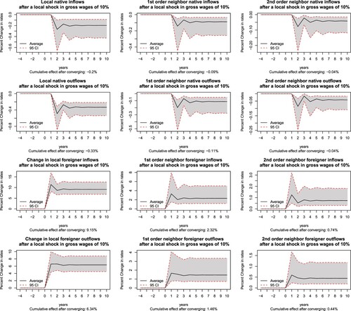
Figures 4–6, respectively, simulate and trace the impacts on the German and the foreign workforce migration flows after a shock in GDP, unemployment or wages. The shocks are applied to each variable locally and are set to 10%. Each graph tracks the local impact, as well as the impact from a local area change onto first- and second-order neighbours. Importantly, the local areas are excluded from the latter.¹⁷ Again we emphasize that the model is applied to total in- and out-migration rates, and not on origin–destination flows. Future analyses could apply our impulse–response techniques to trace interactions at that level. The y-axes of the graphs show the percentage change in the response variable, following the initial change in one of the economic variables.

Figure 4. Estimated impulse–responses.

Note: Changes in gross domestic product (GDP) per capita at the different spatial units (spatial lag = 0, spatial lag = 1, spatial lag = 2). The shaded area represents the confidence bands, using bootstrap estimated of the standard errors obtained by simulation of 1000 replications of the process, each time drawing parameters and innovations from the estimated distributions.

Estimated impulse response of German and foreign workforce migration flows after a shock in GDP per capita at the different spatial intervals (spatial lag = 0, spatial lag = 1, spatial lag = 2). The shaded area represents the confidence bands, constructed using bootstrap estimates obtained by simulation (1000 replications). The figure highlights that different types on migration flows react differently to a drop in GDP per capita.

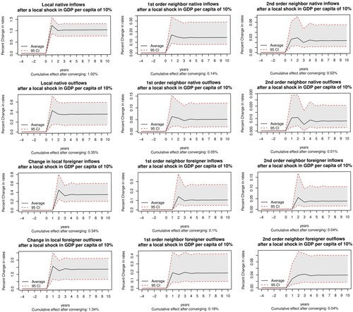
Figure 5. Estimated impulse–responses.

Note: Changes in unemployment rate at the different spatial units (spatial lag = 0, spatial lag = 1, spatial lag = 2). The shaded area represents the confidence bands, using bootstrap estimated of the standard errors obtained by simulation of 1000 replications of the process, each time drawing parameters and innovations from the estimated distributions.

Estimated impulse response of German and foreign workforce migration flows after a shock in employment rates at the different spatial intervals (spatial lag = 0, spatial lag = 1, spatial lag = 2). The shaded area represents the confidence bands, constructed using bootstrap estimates obtained by simulation (1000 replications). The figure highlights that different types on migration flows react differently to a drop in employment rates.

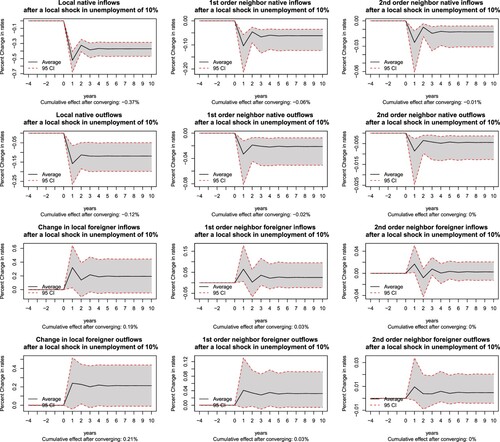
Figure 6. Estimated impulse–responses.

Note: Changes in gross wages at the different spatial unites (spatial lag = 0, spatial lag = 1, spatial lag = 2). The shaded area represents the confidence bands, using bootstrap estimated of the standard errors obtained by simulation of 1000 replications of the process, each time drawing parameters and innovations from the estimated distributions.

Estimated impulse response of German and foreign workforce migration flows after a shock in wage levels at the different spatial intervals (spatial lag = 0, spatial lag = 1, spatial lag = 2). The shaded area represents the confidence bands, constructed using bootstrap estimates obtained by simulation (1000 replications). The figure highlights that different types on migration flows react differently to a drop in wage levels.

Interesting results emerge. For example, Figure 4 shows that a 10% positive shock to GDP per capita is estimated to have positive effects on all types of flows. In simple terms, the model suggests that increased economic growth leads to increased relocation of the workforce, while economic slowdown results in less overall movement. This is a plausible result, as, in a growing economy, an increased number of opportunities may arise, and so people may move more often as a pure result of welfare maximization. The net impact of local GDP growth on net local flows highly depends on the composition of the local workforce. As an example, the estimated long-run effect on German inflows is approximately 1%, with additional economically significant impacts on the directly surrounding areas. Outflows of the German workforce increase only by about 0.35%, and so the German workforce increases on a net basis. The inflow of foreigners increases only by 0.34%, while foreigner outflow increases by 1.34%. This means that the foreign workforce shrinks on a net basis in areas that grow faster. Combined, GDP growth is associated with a net replacement of the foreign workforce by the German workforce, while the net balance of inflows and outflows depends on the initial composition of workforce migration. In areas with large native flows compared with foreigner flows, a small percentage in the first may result in larger flow changes than a larger percentage impact on the latter.

The same analysis for unemployment impacts similarly reveals differential impacts on German and foreign migration flows. An increase in unemployment slows down the inflow of Germans by −0.37% in the long run. Again, there are spatial spillover impacts, but the economic significance of spillovers directly from one area to a single neighbour is small. Outflow also shrinks, but by a smaller amount. This suggests that, on a net basis, rising unemployment has a negative impact on the size of the regional German workforce. The impact on the foreign workforce reacts in an opposite manner. The in- and outflow of the foreign workforce both tend to react positively to rising unemployment, but the estimated long-run effects both have a zero value within their estimated 95% confidence interval (CI). Some evidence for a short-term significant increase in foreigner inflows is found, but it is rather negligible. Taken together, the results suggest that an increase in unemployment is associated with a net outflow of the German workforce and with a positive short-term but negligible long-term impact on the foreign workforce.

Our third simulation study traces the migration flows after wage changes. A decrease in wages is associated with a reduction in German flows. The long-term reduction in German outflows is slightly stronger (−0.33%) than it is for inflows (−0.2%), but the impacts remain significant for spatial neighbours. Taken together, the result suggests that falling wages will lead to a reduction in German newcomers to the regional labour market by acting negatively in the pull factor of the region while simultaneously slowing German (for instance by limiting the financial resources and opportunities needed to move). Falling wages lead to more considerable impacts on the flows of foreigners. The foreign inflow increases by 9.15% in the long term, while outflows increase by −6.34%. Even for higher order neighbours the impact remains significant. This indicates that falling wages lead to a net increase in the foreign workforce.

5.3. Implications for resilience policies

The direction if impacts are clear. If rising unemployment coincides with falling GDP and falling wages, the effects of the three equations compound and lead to an increased share of foreigners relative to natives in the workforce. While the model does not explicitly model price dynamics, and does not provide a granular explanation for these patterns, it is plausible that the main estimated dynamics are driven by impacts on purchasing power. In particular, regionally falling wages may reduce the purchasing power of the local population. This could cause a part of the German workforce that is able, to leave in pursuit of higher wages elsewhere, while a large part that may no longer be able to purchase similar quantities of goods elsewhere, decides to stay. At the same time, reduced price levels may make the area more affordable to foreigners who currently live and work elsewhere, leading to an increased inflow. This also highlights that the estimated differences in migration responses resulting from the native-foreign distinction may reflect differences in responses over an income distribution with higher worth individuals reacting differently to economic events from those below median income.

Whether adverse economic events result in net outflows of the workforce or only in a redistribution of subpopulations depends on the initial composition of workforce migration. Moreover, the long-term economic consequences of the migration patterns may depend on an area’s ability to provide increased opportunity for economic activity to the newcomers relative those who left. In those areas where newcomers do not find opportunities to engage in economic production, unemployment may rise further and GDP pay fall further, reinforcing the economic dynamic. In other areas where newcomers assimilate well into the workforce, GDP may rise while unemployment may fall. Ultimately, the balance of all effects may be the result of more nuances. For example, an increase in GDP may occur alongside a reduction in unemployment and an increase in wages. The first two events are associated with increased inflows of the German workforce, and so they would strengthen one another. The increased wages statistically slow down additional inflows, which, again, may be related to increasing price levels that occur alongside growth in disposable income. The total impact on the inflow of the German workforce would thus vary by the extent to which GDP growth and unemployment reductions occur relative to wage and price levels.

Clearly, in an ideal setting, policymakers could anticipate the local effects and inform their local labour market policies on the basis of simple generalizations that draw from what has occurred elsewhere. So far, the results suggest that the migration responses in any one area following an economic event are likely highly specific to the area. Apart from the initial composition of workforce migration, and the effects of GDP and unemployment changes relative to wage changes, another complication lies in the substantial spatial interaction components captured in the model. Net impacts may be further compounded by spatial spillovers. Even though the impulse–response function (IRF) results suggest that the effect of spatial spillovers, measured directly from one area to the next, is often not very high, the total economic significance of combined spatial spillovers may be substantial and often outweigh local impacts in our data.¹⁸ This highlights that, apart from the role that local conditions play in shaping the migration and economic consequence of an initial economic shock, the regional conditions may play an even larger role. This suggests that local communities should likely develop their resilience plans in coordination with neighbours.

6. CONCLUSIONS

Migration dynamics are shaped by the relative positioning of complex economies in a geographic context, and driven by a large spectrum of shocks. In order to analyse why certain areas are more resilient to initial economic shocks, one may view migration dynamics through a lens of spatially varying population compositions that each follow different migration dynamics, and whose movements result in different economic impacts. This paper has empirically investigated the internal migration patterns of both the domestic and the foreign population using data from Germany during a multi-year period that also includes the European recession years.

Though there is a large body of literature focusing on German internal migration, this paper presents a unique combination of multivariate time–space dynamics. The backbone of the model adopted here follows a time-series VAR structure that allows the direction of causality to be investigated by utilizing the arrow of time. Following recent advances in spatial time-series literature, we extended the VAR model to include spatial autocorrelation. We estimated the model using maximum likelihood and used the estimated parameter distributions to perform a stochastic impulse–response simulation.

Our study addresses internal migration of both Germans and foreigners, but it is important to highlight that our data does not explicitly capture, nor seeks to explain, differences in these populations. This means that the differences in migration behaviour arising from the native-foreign distinction may relate to nonlinearities that vary smoothly over the income distribution. It is left to future research to tackle this explicitly, but our background discussion pointed towards several papers that have more explicitly looked into the role of ethnic–cultural compositions in migration. In addition, the model captures GDP, unemployment and wages, but does not capture prices. Earlier work has, for example, already stressed the importance of house prices. In our data, increases in wages may occur alongside increases in price levels, which in turn may be an important push or pull factor through changes in purchasing power.

Our parameter estimates confirm neo-classical dynamics to hold in Germany, as found by earlier studies. The impulse–response analysis produced several interesting empirical results that highlight differences in the push and pull factors that drive flows of natives and foreigners. Declining GDP, rising unemployment and falling wages, act positively on the relative share of foreign workers in local areas, but the results highlight that the impact varies based on how GDP growth and unemployment changes relative to wages. Moreover, the impacts on net migration flows depend heavily on the initial composition of workforce migration specific to that area. The economic consequences of migration may depend on an areas ability to provide economic opportunity to newcomers, relative to those that left, with possibilities for reinforcing dynamics. The estimates also showed a high degree of spatial spillovers, with cumulative regional effects likely outweighing local effects in most cases.

The results on Germany provide important clues for understanding differences in local economic resilience that are rooted in geographical contexts, and highlight the importance of a place-based approach to policy within a regional framework: the consequences of an economic shock are highly place specific, group specific and dependent on how neighbours cope with the same shock. Therefore, there is a need for local policy interventions aimed at mitigating the impacts of economic shocks that take into account the place-specific socio-economic circumstances that are unique to an area, but such localized efforts should be supported regionally due to their wider regional benefits.

DISCLOSURE STATEMENT

No potential conflict of interest was reported by the authors.

Additional information

Funding

Peter Nijkamp acknowledges the receipt of a grant from the Ministry of Research, Innovation and Digitization (Romania) [project number PN III-P4-PCE-2021-1878]. Masood Gheasi acknowledges support from the UKRI [fund number MR/S032711/1].

Notes

1. It is noteworthy that Parikh and Leuvensteijn (2003) tried to explain German internal migration after reunification not only through the lens of wage differences and the unemployment rate, but also by including additional variables such as regional housing prices, geographical distance and inequality measures.

2. To our knowledge, only two publications, Möller (1995) and Mitze and Reinkowski (2011), apply a VAR methodology to German internal migration flows. Möller (1995) applied a VAR model for seven West German regions for the years 1960–93, and found a negative impulse–response from unemployment shocks on migration. Mitze and Reinkowski (2011) studied East–West migration from 1991 to 2006 and applied a dynamic panel data method in a VAR setting. Furthermore, they found that regional disparities in real wage and unemployment rates work as dominant push and pull factors of internal migration in Germany. They also confirmed the finding from the neoclassical theory of migration that migration has an equilibrating effect on regional labour markets. The spatial structure adopted here allows our paper to provide two unique combinations relative to these previous studies: (1) we consider Germany as a whole, allowing spillovers to travel between East and West, while previous studies on German internal migration mainly focused either on West Germany or on East to West German migration; and (2) the present study focuses on the migration interactions between Germans and foreign-born people, so that we also address segmented labour mobility in a spatially connected network in which local areas are not treated as being isolated from others.

3. Counties are the equivalents of the third layer of the Nomenclature of Territorial Units in Statistics (NUTS-3).

4. The Federal Statistical Office defines foreigners as all people who are not Germans. This includes anyone who has a foreign citizenship (including asylum seekers and refugees), while Germans who also have a foreign citizenship are considered Germans rather than foreigners.

5. An example for the latter case is given by change in delineations that took place in Saxony in 2008, where two or more existing counties were merged to form a new county.

6. This is the case when an existing county is split up and assigned in parts to two different new counties. Such changes in delineations occurred during the county reforms of Saxony-Anhalt (2007) and Mecklenburg-Vorpommern (2013). The excluded counties are (county ID in parentheses): Dessau-Rosslau (15001); Landkreis Anhalt-Bitterfeld (15082); Landkreis Jerichower Land (15086); Salzlandkreis (15089); Landkreis Wittenberg (15091); Mecklenburgische Seenplatte (13071); and Landkreis Vorpommern-Greifswald (13075).

7. Economic data including those on annual GDP per capita and annual disposable income per capita are notoriously difficult to be assigned to lower level geographical entities. We have to take the quality of the data for granted but remind the reader that there may be uncertainties in the underlying datasets. In the specific case of the annual GDP and annual disposable income, computation is undertaken by the Federal Statistical Office and the statistical offices of the federal states. The approach taken to construct GDP at the county (NUTS-3) level is based on a top-down approach that involves distributing the value of GDP at the federal state (NUTS-1) level across the counties within that federal state. This is done by means of the regional sectoral structure at the two-digit level. The Federal Statistical Office provides further details on the construction of these variables (in German only) at https://www.statistikportal.de/de/vgrdl/methoden-und-informationen. Data on the regional unemployment rates, by contrast, are based on administrative statistics from the Federal Employment Agency. As these statistics are based on the registrations of the universe of employed and unemployed individuals, the data can be deemed highly reliable.

8. This multivariate strategy differs from the seemingly unrelated regression (SUR) model used by Grossman (1982) to study the elasticity of substitution between native and migrant workers using cross-sectional data in the United States. In particular, the VAR focuses on multivariate interaction over the time dimension, while the SUR estimates instantaneous cross-equation correlations over the cross-section. The VAR approach naturally only becomes interesting when data are available for multiple consecutive periods, but then allows inferring the order in which separate processes influence each other over time. The Sp-VAR application further differs from the time-series extension of the gravity model as explored by Plane et al. (1984), which could be estimated similarly with spatial interaction (thereby considering instantaneous dependence between the flows of connected origin–destination pairs) by focusing instead on the total in- and out-migration rates of NUTS-3 areas.

9. Structural modelling with the Sp-VAR is discussed by Giacinto (2010), while Andrée et al. (2019) investigate an Sp=VAR extension that includes cross-equation moving averages. The latter paper points out that the Sp-VAR is a restricted simultaneous interdependent multiple equation model where the structure of restrictions results from the specification of the spatial weights matrices. The Sp-VAR can be inverted and approximated by a Sp-VMA model and inclusion of moving average components in the Sp-VAR model can improve specification, but estimating moving average components is complicated by the fact that multiple solutions to the likelihood function may exist. Moreover, the moving average components have to be initialized across the entire cross-section, and so the initialization remains influential when $N>>T$, which makes estimating pure Sp-VAR dynamics more straightforward in the setting of the current paper.

10. Stationarity of each spatial time series $\{Y_k{\}}_t^T$ was rejected in our analysis using a Dickey–Fuller (DF) test with trend and constant. After rejecting stationarity, all variables are transformed into rates of change and the DF statistics did not reject stationarity.

11. We used only the first-order contiguity weights matrix, as Stakhovych and Bijmolt (2009) indicate that in a Monte Carlo simulation the first-order contiguity weights matrix performs better, on average, than those using the K-nearest neighbour and inverse distance weights matrices. Ultimately, this may depend on the application, but a simple Taylor expansion around the spillovers highlights that, with a contiguity matrix, spillovers can travel far across the spatial system before effects die out and so the shape of the spatial response function follows that of an inverse distance decay function.

12. It should be added that, in principle, it might be possible to differentiate the two population groups native and foreign residents into geographical cohorts and then estimate the equations of the Sp-VAR model using quantile regression methods (see also McMillen, 2012). Notwithstanding the methodological attractions of this approach, this would require an extensive data conversion and collection effort, with most likely interesting results. This could then be part of a follow-up study. In that regard, the smooth transition spatial autoregressive model of Andrée et al. (2017) would also provide interesting opportunities to model threshold dynamics in dependencies, allowing for dependencies in migration processes to change sharply or smoothly around tipping points.

13. This is done by randomly drawing innovations from the estimated error distributions and generating hypothetical future values for the process at its estimated parameter values. Each time, after 50 burn-in simulation steps, the simulated process is forked into two simulations, both carried forward using identical innovations. Only to one version of the processes is a shock applied to one input variable in a randomly drawn location, while the other version of the process is carried forward without applying that shock. The difference between the perturbed and unperturbed process is then calculated at each simulated time step. The stochastic impulse–response simulation is repeated 1000 times, each time drawing parameter values from the estimated parameter distributions to account for uncertainty in the model’s estimated parameter values. Each simulation applies the shock locally to one randomly selected unit in the cross-section, and the divergence between the perturbed and the unperturbed system can then be tracked at that location, but also at neighbours in order to understand the magnitude of spatial spillovers. After 1000 of such stochastic shock–response simulations have been performed, an average impulse–response path is calculated locally and at (higher order) neighbours along with quantiles to indicate uncertainty.

14. This still means that for an initial shock in variable $Y_{k,t}$ at time $t$, there can be multiple subsequent effects that occur simultaneously at time $t+2$. For example, $Y_{k,t+2}$ can be influenced simultaneously through multiple transmission channels; variables $Y_{k\in 1,\dots K,t+1}$ that may have been impacted by the initial shock in $Y_{k,t}$.

15. Adding additional weights matrices that capture direct connections between distant areas could be a future extension to improve the model fit, but would also add complexities that make the overall spillover dynamic captured by the model difficult to comprehend. We also note that the statistical exploration of the flows might alternatively be based on destination competition using hierarchical choice models (Fotheringham, 1986).

16. Additional simulation results are available from the authors upon request.

17. Strictly speaking, each area is a second-order neighbour to itself.

18. Recall that the average district has eight neighbours, and so the cumulative impact of first-order spillovers is on average eight times the estimated long-run impact on a single district. As an example, simplifying again to the extent that a GDP shock is considered in isolation, the local inflow of the German workforce increases by 1.02% after a 10% increase. If that area has eight neighbouring districts, one may expect that the inflow in the directly surrounding areas increases by 0.14% in all eight districts. On a rectangular grid, the total number of second-order neighbours would be 24, and so the expected 0.02% increase in these more distant areas occurs, on average, another 24 times. If all areas were identical, the total change in inflow in the region excluding local changes would outweigh the change in local flows by a factor of almost 1.6. Note that the concept of spatial connectedness is here based on that of contiguity which is an over-simplification of a more complex concept of connectedness that in reality may depend on many conditions specific to an area.

REFERENCES

- Andrée, B. P. J. (2019). Probability, causality and stochastic formulations of economic theory. SSRN Electronic Journal. https://doi.org/10.2139/ssrn.2977830
- Andrée, B. P. J. (2020). Theory and application of dynamic spatial time series models. Rozenberg and Tinbergen Institute.
- Andrée, B. P. J. (2022). Conducting causal analysis by means of approximating probabilistic truths. Entropy, 24(1), 92. https://doi.org/10.3390/e24010092
- Andrée, B. P. J., Blasques, F., & Koomen, E. (2017). Smooth transition spatial autoregressive models. Tinbergen Institute Discussion Papers TI 2017-050/III. https://doi.org/10.2139/ssrn.2977830
- Andrée, B. P. J., Spencer, P., Chamorro, A., Wang, D., Azari, S. F., & Dogo, H. (2019). Pollution and expenditures in a penalized vector spatial autoregressive time series model with data-driven networks. World Bank Policy Research Working Papers, 8757. https://doi.org/10.1596/1813-9450-8757
- Anselin, L., & Griffith, D. A. (1988). Do spatial effects really matter in regression analysis? Papers in Regional Science, 65(1), 11–34. https://doi.org/10.1111/j.1435-5597.1988.tb01155.x
- Beck, G. (2011). Wandern gegen den strom [Doctoral dissertation]. FU Berlin. https://doi.org/10.17169/refubium-11062
- Beenstock, M., & Felsenstein, D. (2019). The econometric analysis of non-stationary spatial panel data. Advances in spatial science. Springer.
- Bilger, U., Genosko, J., & Hirte, G. (1991). Migration and regional labour market adjustment in West Germany. In Stillwell J., & Congdon, P. (Eds.), Migration models: Macro and micro approaches (pp. 152–167). London.
- Borjas, G. J., Freeman, R. B., Katz, L. F., DiNardo, J., & Abowd, J. M. (1997). How much do immigration and trade affect labor market outcomes? Brookings Papers on Economic Activity, 1997(1), 1–90. https://doi.org/10.2307/2534701
- Börsch-Supan, A., Härtl, K., & Ludwig, A. (2014). Aging in Europe: Reforms, international diversification, and behavioral reactions. American Economic Review, 104(5), 224–229. https://doi.org/10.1257/aer.104.5.224
- Bröcker, J., & Mitze, T. (2020). Factor mobility and migration models. In Handbook of regional science (pp. 349–372). Springer. http://doi.org/10.1007/978-3-662-60723-7_42
- Brunetta, G., & Caldarice, O. (2020). Spatial resilience in planning: Meanings, challenges, and perspectives for urban transition. In Leal Filho, W., Marisa Azul, A., Brandli, L., Gökçin Özuyar, P., & Wall, T. (Eds.), Sustainable cities and communities. Encyclopedia of the UN Sustainable Development Goals. Springer. https://doi.org/10.1007/978-3-319-95717-3_28
- Burda, M. C., & Hunt, J. (2001). From reunification to economic integration: Productivity and the labor market in eastern Germany. Brookings Papers on Economic Activity, 2001(2), 1–92. https://doi.org/10.1353/eca.2001.0016
- Carlino, G. A., & Mills, E. S. (1987). The determinants of county growth. Journal of Regional Science, 27(1), 39–54. https://doi.org/10.1111/j.1467-9787.1987.tb01143.x
- Chun, Y. (2008). Modeling network autocorrelation within migration flows by eigenvector spatial filtering. Journal of Geographical Systems, 10(4), 317–344. https://doi.org/10.1007/s10109-008-0068-2
- Chun, Y., & Griffith, D. A. (2011). Modeling network autocorrelation in space–time migration flow data: An eigenvector spatial filtering approach. Annals of the Association of American Geographers, 101(3), 523–536. https://doi.org/10.1080/00045608.2011.561070
- Clemens, M. A. (2016). Losing our minds? New research directions on skilled emigration and development. International Journal of Manpower, 37(7), 1227–1248. https://doi.org/10.1108/IJM-07-2015-0112
- Decressin, J. (1994). Internal migration in west Germany and implications for East–West salary convergence. Review of World Economics, 130(2), 231–257. https://doi.org/10.1007/BF02707708
- Elhorst, J. P. (2010). Spatial econometrics: From cross sectional data to spatial panels. Springer.
- Fotheringham, A. S. (1986). Modelling hierarchical destination choice. Environment and Planning A, 18(3), 401–418. https://doi.org/10.1068/a180401
- Friedrich, K. (2008). 16 jahre innerdeutsche Ost–West-Migration – eine Einführung in die Transformation eines geschlossenen Migrationsregimes in die Postmoderne. Brain drain oder brain circulation, 13–20.
- Giacinto, V. (2010). On vector autoregressive modeling in space and time. Journal of Geographical Systems, 12(2), 125–154. doi: 10.1007/s10109-010-0116-6
- Gløersen, E., Druagulin, M., Hans, S., Kaucic, J., Schuh, B., Keringer, F., & Celotti, P. (2016). The impact of demographic change on European regions. European Union, Committee of the Regions, fecha de consulta, 10(10), 2016. https://policycommons.net/artifacts/2017730/the-impact-of-demographic-change-on-european-regions/2770172/ on 19 Mar 2023. CID: 20.500.12592/bd1xf7
- Granger, C., King, M. L., & White, H. (1995). Comments on testing economic theories and the use of model selection criteria. Journal of Econometrics, 67(1), 173–187. https://doi.org/10.1016/0304-4076(94)01632-A
- Grossman, J. B. (1982). The substitutability of natives and immigrants in production. The Review of Economics and Statistics, 64(4), 596–603. https://doi.org/10.2307/1923944
- Harris, J. R., & Todaro, M. P. (1970). Migration, unemployment and development: A two-sector analysis. The American Economic Review, 60(1), 126–142. https://www.jstor.org/stable/1807860
- Heiland, F. (2004). Trends in East–West German migration from 1989 to 2002. Demographic Research, 11, 173–194. https://doi.org/10.4054/DemRes.2004.11.7
- Hunt, J. (2000). Why do people still live in East Germany? (Technical Report). National Bureau of Economic Research (NBER).
- Jurjevich, J. R., & Plane, D. A. (2012). Voters on the move: The political effectiveness of migration and its effects on state partisan composition. Political Geography, 31(7), 429–443. https://doi.org/10.1016/j.polgeo.2012.08.003
- Kondoh, K. (2017). The economics of international migration. Environment, Unemployment. Springer Science+Business Media. 10.1007/978-981-10-0092-8
- Kontuly, T., Vogelsang, R., Schön, K. P., & Maretzke, S. (1997). Political unification and regional consequences of German east–west migration. International Journal of Population Geography, 3(1), 31–47. https://doi.org/10.1002/(SICI)1099-1220(199703)3:1<31::AID-IJPG54>3.0.CO;2-G
- LeSage, J. P., & Fischer, M. M. (2010). Spatial econometric methods for modeling origin–destination flows. In Fischer, M., & Getis, A. (Eds.), Handbook of applied spatial analysis. Springer. https://doi.org/10.1007/978-3-642-03647-7_20
- Lu, M. (2001). Vector autoregression (VAR): An approach to dynamic analysis of geographic processes. Geografiska Annaler: Series B, Human Geography, 83(2), 67–78. https://doi.org/10.1111/j.0435-3684.2001.00095.x
- Luthra, R., Platt, L., & Salamońska, J. (2016). Types of migration: The motivations, composition, and early integration patterns of new migrants in Europe. International Migration Review, 52. https://doi.org/10.1111/imre.12293
- Martin, R., & Sunley, P. (2015). On the notion of regional economic resilience: Conceptualization and explanation. Journal of Economic Geography, 15(1), 1–42. https://doi.org/10.1093/jeg/lbu015
- Massey, D. S., Arango, J., Hugo, G., Kouaouci, A., Pellegrino, A., & Taylor, J. E. (1993). Theories of international migration: A review and appraisal. Population and Development Review, 19(3), 431–466. https://doi.org/10.2307/2938462
- McMillen, D. P. (2012). Quantile regression for spatial data. Springer Science.
- Meen, G. (2016). Spatial housing economics: A survey. Urban Studies, 53(10), 1987–2003. https://doi.org/10.1177/0042098016642962
- Michelsen, C., & Weiß, D. (2010). What happened to the East German housing market? A historical perspective on the role of public funding. Post-Communist Economies, 22(3), 387–409. https://doi.org/10.1080/14631377.2010.498686
- Mitze, T., & Reinkowski, J. (2011). Testing the neoclassical migration model: Overall and age-group specific results for German regions. Zeitschrift für ArbeitsmarktForschung, 43(4), 277–297.
- Möller, J. (1995). Empirische Analyse der Regionalentwicklung. Regensburger Diskussionsbeiträge zur Wirtschaftswissenschaft, 271, Working Paper.
- Napolitano, O., & Bonasia, M. (2010). Determinants of different internal migration trends: The Italian experience. MPRA, Paper No. 21734. https://mpra.ub.uni-muenchen.de/21734/
- Nijkamp, P., & Poot, J. (2015). Cultural diversity: A matter of measurement. In P. Nijkamp, J. Poot & J. Bakens (Eds.), The economics of cultural diversity (pp. 17–51). Edward Elgar.
- Parikh, A., & Leuvensteijn, M. V. (2003). Interregional labour mobility, inequality and wage convergence. Applied Economics, 35(8), 931–941. https://doi.org/10.1080/0003684022000035827
- Partridge, M. D., & Rickman, D. S. (2006). An SVAR model of fluctuations in US migration flows and state labor market dynamics. Southern Economic Journal, 72(4), 958–980. https://doi.org/10.1002/j.2325-8012.2006.tb00748.x
- Pascariu, G. C., Banica, A., & Nijkamp, P. (2022). A meta-overview and bibliometric analysis of resilience in spatial planning the relevance of place-based approaches. Applied Spatial Analysis and Policy, 1–31. https://doi.org/10.1007/s12061-022-09449-z
- Peng, C.-W., & Tsai, I.-C. (2019). The long- and short-run influences of housing prices on migration. Cities, 93, 253–262. https://doi.org/10.1016/j.cities.2019.05.011
- Plane, D., Rogerson, P., & Rosen, A. (1984). The cross regional variation of inmigration and outmigration. Geographical Analysis, 16(2), 162–175. https://doi.org/10.1111/j.1538-4632.1984.tb00808.x
- Schneider, H. R., & Rinne, U. (2019). The labor market in Germany, 2000–2018. IZA World of Labor 379. doi: 10.15185/izawol.379.v2
- Schneider, L. (2005). Ost–West-Binnenwanderung: Gravierender Verlust an Humankapital. Wirtschaft im Wandel, 11(10), 308–314. http://hdl.handle.net/10419/143420
- Schoeni, R. F. (1997). New evidence on the economic progress of foreign-born men in the 1970s and 1980s. Journal of Human Resources, 32, 683–740. https://doi.org/10.2307/146426
- Schultz, A. (2009). Forschungen zur deutschen landeskunde. In Brain drain aus Ostdeutschland (pp. 258–276). Selbstverlag der Deutschen Akademie für Landeskunde.
- Sims, C. A. (1972). Money, income, and causality. The American Economic Review, 62(4), 540–552. https://www.jstor.org/stable/1806097
- Sin, C.-Y., & White, H. (1996). Information criteria for selecting possibly misspecified parametric models. Journal of Econometrics, 71(1), 207–225. https://doi.org/10.1016/0304-4076(94)01701-8
- Stakhovych, S., & Bijmolt, T. H. A. (2009). Specification of spatial models: A simulation study on weights matrices. Papers in Regional Science, 88(2), 389–408. https://doi.org/10.1111/j.1435-5957.2008.00213.x
- Tanis, K. (2020). Regional distribution and location choices of immigrants in Germany. Regional Studies, 54(4), 483–494. https://doi.org/10.1080/00343404.2018.1490015
- Wang, D., Andrée, B. P. J., Chamorro, A. F., & Spencer, P. G. (2022). Transitions into and out of food insecurity: A probabilistic approach with panel data evidence from 15 countries. World Development, 159, 106035. https://doi.org/10.1016/j.worlddev.2022.106035
- Weidlich, W., & Haag, G. (1988). Interregional migration: Dynamic theory and comparative analysis, Vol 4. Springer.
- Wixe, S., & Andersson, M. (2017). Which types of relatedness matter in regional growth? Industry, occupation and education. Regional Studies, 51(4), 523–536. https://doi.org/10.1080/00343404.2015.1112369