Keep calm and carry on emitting: cap-and-trade rules, local emissions and growth

ABSTRACT

We estimate the impact of the Cap-and-Trade Program (CATP) in California on regional greenhouse gas emissions and economic growth. Our preferred identification strategies, based on spatial distance and county-level contiguity, fail to provide evidence of a reduction in regional emissions or economic growth due to the CATP. Multi-state organisations do not transfer emissions to non-Californian facilities, but parent-level concentration in emissions changes, consistent with an insofar unexplored form of regulatory arbitrage. Overall, our results highlight the importance of a regional approach when designing climate policies and evaluating their effects.

KEYWORDS:

• economic growth
• regional contiguity
• CO₂ emissions
• climate policy

JEL:

• G18
• Q50
• Q52
• Q58
• R0
• R11

1. INTRODUCTION

Climate change is one of the most important challenges of our time – as demonstrated by the media hype around the latest Conferences Of the Parties (particularly, COP26 and COP27) – and has attracted widespread commitment to curb greenhouse gas (GHG) emissions from politicians worldwide. For instance, the Kyoto Protocol (never ratified by the United States) and the more recent 2016 Paris Agreement represent large-scale commitments to mitigate GHG emissions (Bonnett & Birchall, 2022). The European Union Emissions Trading System (EUETS) – arguably one of the largest programmes in the world – is a good example of how those commitments are turned into actions. In addition to these super-national policies, there have also been regional initiatives aiming to attain both economic and environmental goals. Against this backdrop, a policy debate has thus arisen on the effectiveness of climate policy regulations and their economic effects at the regional level (Baldwin & Wing, 2013). In fact, recent evidence regarding the success of such policies is mixed (Gibbs & Jensen, 2022), and global emissions have continued to rise in the past decades (Bonnett & Birchall, 2022; Cojoianu et al., 2021).

In this paper, we assess the regional impact of the Cap-and-Trade Program (CATP) introduced in California in 2013. In particular, we investigate whether the Californian CATP – for which we provide a detailed institutional background in section A in Appendix A in the supplemental data online – leads to a reduction in GHG emissions, and if such reduction (if any) is accompanied by lower local economic growth. In follow-up analyses, we also explore the behaviour of multi-state organisations owning facilities in and out of California. We focus on the Californian CATP because its application lends itself to a robust identification strategy based on a difference-in-differences (DiD) approach, where California is the treatment state and other states are used as control. Particularly, the contiguous states (i.e., Arizona, Oregon, Nevada) are unlikely to be affected by regulations that are similar to the Californian CATP during the period under examination. Indeed, despite being one of the promoters, Arizona withdrew from the Western Climate Initiative (which is another cap-and-trade system), before it even started, in 2011.¹ Equally, Oregon and Nevada were not involved in analogous schemes during our sample period.^2,3 We contribute to the existing literature on the CATP by focusing on its regional effects, using counties as the main unit of analysis.⁴ This is important because there is substantial heterogeneity in within-state county-level growth, and therefore focusing on state-level economic growth misses important variation at the local level.

The granularity of the data at our disposal enables us to answer our research questions using a variety of identification strategies. Specifically, we employ county-level data on gross domestic product (GDP) – recently made available by the Bureau of Economic Analysis (BEA) – for specifications based on all counties in California and its adjacent states, and only contiguous counties which lie at the border between California and neighbouring states (Oregon, Nevada and Arizona). Regional contiguity ensures that the treatment and control samples are as close as possible in terms of economic and demographic characteristics (Egger & Lassmann, 2015). This is particularly important when studying the consequences of GHG emissions because contiguous regions are more likely to have a similar climate than regions far apart, and there is a link between local climate and GHG emissions (Yuksel & Michalek, 2015). In particular, local rainfall and temperature can influence GHG emissions (Borck, 2016; Borenstein et al., 2019).⁵

In addition to county-level data, we exploit facility-level data to explore the impact of the CATP on investment policies. Specifically, we match the facility-level data with information on the parent organisations owning the facilities to test whether the CATP led to transfers of emissions from facilities in California to facilities in other states – a phenomenon known as ‘leakage’ (see, inter alia, Cui et al., 2017).⁶ Moreover, we examine if organisations owning the facilities sell all or part of their ownership shares in Californian counties as a consequence of the CATP.

The remainder of the paper is structured as follows. The next section offers an overview of several strands of the regional literature on climate policies and discusses our contribution to each of these strands. Section 3 describes our data and methodology. Section 4 presents our main findings, while section 5 investigates a potential underlying mechanism. Section 6 discusses policy implications and section 7 concludes.

2. RELATED LITERATURE AND CONTRIBUTION

Our paper extends the literature on carbon market trading, which encompasses studies on the EUETS (e.g., Knight, 2011). Commonly debated in this area are the decisions regarding the emissions cap (i.e., the maximum level of GHG emissions companies can produce, which can be subject to regulatory capture) and other unintended consequences of cap-and-trade systems, such as pollution leakage. Such a phenomenon occurs when organisations transfer emissions outside of the jurisdiction that is imposing a cap on pollution generation rather than meeting environmental reductions. If this occurs, pollution taxes applied in one region lead to increased emissions in other regions, especially when dirty industries change location. As noted by Cui et al. (2017), there is also a relationship between economic growth and emissions leakage. Intuitively, if dirty industries are significant drivers of the local economy of a region, the introduction of an emissions cap might result in lower local economic growth. However, in the absence of regulatory constraints, firms might transfer the emissions in excess of the cap to unregulated regions, especially if they own similar facilities, or the cost of converting existing facilities or building new ones in unregulated regions is low. Overall, this corroborates the view of Weller (2012), who underscores the regional implications that carbon-mitigation policies can have and which need to be taken into account when designing a cap-and-trade system. In addition to pollution leakage, emitters can engage in regulatory arbitrage by reducing their ownership share of facilities in regulated regions only to increase it in unregulated regions, thereby keeping their overall contribution to emissions at the aggregate level unchanged. This behaviour leads to a change in the ownership concentration of emissions in regulated regions compared to unregulated ones. However, to the best of our knowledge, no study has investigated this type of regulatory arbitrage.

Critics of cap-and-trade systems have also pointed out the possibility of regulatory capture. Substantial lobbying activities from large corporations may result in a non-binding emission cap – despite counteracting lobbying activities from environmental groups (Adam, 2011)⁷ – undermining the effectiveness of the cap-and-trade mechanism. While we cannot provide direct evidence of regulatory capture, we nonetheless assess whether the implementation of the Californian CATP achieves the goal of emissions reduction and whether this affects regional economic growth. In follow-up analyses, we also test whether the adoption of such a carbon trading scheme results in emissions leakage. Finally, and more importantly, we test if the CATP gives room for a reshuffling of ownership concentration of emissions.

Our contribution is important because recent studies on the impact of climate policies on economic growth tend to concentrate on national (Granados & Spash, 2019) or state-level GDP data (Bartram et al., 2022). The focus on state-level GDP data is, at least partly, due to a lack of county-level GDP data for the United States until recently, and extends beyond the analysis of climate regulation. For example, in the literature about tax policies (Biswas et al., 2017; Liu & Williams, 2019) the focus tends to be on state-level GDP growth. Unlike these papers, we use county-level GDP data from the BEA, which was unavailable until late 2019. Such a regional perspective is important because it enables a more precise estimation of the effects of energy production at the local level (Feyrer et al., 2017; Feyrer et al., 2020; James & Smith, 2020).

Our paper is also connected to the literature on the design and impact of regional policies aimed at decreasing GHG emissions without necessarily considering the impact on economic growth. For example, Jones (2019) provides a new framework to assess the application of performance management in city governments in the context of climate change policies. A city-level perspective is justified by the significant contribution of cities to GHG emissions (Acuto, 2016), and the existence of important initiatives by city-mayor networks, such as the C40 Cities Climate Leadership Group (Sancino et al., 2022). In the United States, counties tend to be bigger than cities, but this is not always the case – for example, New York City consists of five counties. Moreover, many facilities in our sample are owned by municipalities. Therefore, we consider a comparable level of granularity to that of studies based on city-level data. In addition, by combining facility-level with ownership-level data to measure local market shares, our granular analysis can provide novel insights to the debate and inform regional policies.

A regional perspective is necessary for the transition to a green economy for several reasons. First, as highlighted by Gibbs et al. (2005), sustainable development strategies are a key part of regional economic strategies that require inter-firm networking (Deutz & Gibbs, 2008), trust and cooperation, along with other elements of the ‘territorial capital’ of a region’s competitiveness (Camagni & Capello, 2013). Second, investigating the interaction between economic and environmental issues at the regional scale can lead to new findings that might help to design a more sustainable and inclusive economic framework (Turok et al., 2017). Third, a regional focus facilitates an experimental approach whereby ‘niche’ developments can be used to test innovative ideas and technologies (Gibbs & O’Neill, 2017). Finally, the symptoms of poor environmental, economic and social policies are more easily evaluated at the regional level than at the national level, and therefore a regional perspective also helps to avoid conflicting agendas between national and regional governments (Heim et al., 2022). By assessing the regional impact of the CATP, we can shed light on potential flaws in climate policies that might remain undetected when considering a national perspective.

3. DATA AND METHODOLOGY

3.1. Data

Similar to recent literature on local economic growth, we focus on GDP per capita (Cermeño, 2019) at the county level. We collect county-level data on real GDP and population (number of individuals residing in a given area) from the BEA.⁸ By employing the income method, the BEA computes county-level GDP as the sum of compensation of employees, taxes on production and imports – less subsidies – and gross operating surplus (Aysheshim et al., 2020).

We retrieve data for the quantity of GHG emissions from the Environmental Protection Agency (EPA) website,⁹ which provides information since 2010 via the GreenHouse Gas Reporting Program (GHGRP). The data are available at the facility level, on a yearly basis, with precise information regarding the geographical location of the facility (i.e., latitude and longitude), as well as parent company ownership. We consider only the years from 2010 to 2015 to avoid the confounding effects of the Paris Accord in 2016. This set-up enables us to study the short-term real effects of the CATP.¹⁰

In our main analysis, we use the natural logarithm of county-level real GDP per capita (calculated as ln[1 + GDP per capita]) as our dependent variable to examine the impact of the CATP on local economic growth. Additionally, we estimate the effect of the programme on total emissions at both the county level – using ln[1 + Emissions per capita] as the dependent variable – and facility-level (ln[1 + Facility emissions]). As reported in note 3, our county-level results remain virtually the same when we do not adjust for county-level population.

In the facility-level regressions, we also allow for the decisions made by the organisation(s) owning the facilities.¹¹ While we run these regressions at the facility level, we consider the impact of time-invariant components related to the parent organisations. We report the definitions of the main dependent variables used in our regressions in Table A1 in Appendix A in the supplemental data online. Table A1 also includes the definitions of other variables which we employ later on in our analysis.

Table 1 reports the summary statistics for our county-level dependent variables, GDP per capita (ln) and Emissions per capita (ln), separately for the whole sample (panel A), counties in California (panel B), counties from the rest of the United States excluding California (panel C), counties in California and contiguous states (Oregon, Nevada and Arizona) (panel D), and contiguous counties at the border between California and Oregon, California and Nevada, and California and Arizona (panel E).

Table 1. Summary statistics for GDP per capita (ln) and Emissions per capita (ln).

	Observations	Mean	SD	P1	P10	P50	P90	P99
(A) All counties
GDP per capita (ln)	18,510	3.6353	0.5374	2.6486	3.0447	3.595	4.1982	5.5000
Emissions per capita (ln)	10,876	2.1316	1.5273	0.0503	0.4646	1.8325	4.3125	6.6303
(B) California = 1
GDP per capita (ln)	348	3.7890	0.3675	3.2437	3.3674	3.6739	4.2060	4.9058
Emissions per capita (ln)	249	1.0651	0.8391	0.1093	0.2284	0.8759	2.1458	4.0123
(C) California = 0
GDP per capita (ln)	18,162	3.6324	0.5397	2.6475	3.0411	3.5930	4.1976	5.5108
Emissions per capita (ln)	10,627	2.1566	1.5309	0.0494	0.4778	1.8643	4.3361	6.6448
(D) California and contiguous states
GDP per capita (ln)	750	3.7805	0.5430	3.0055	3.2825	3.6278	4.3158	6.0868
Emissions per capita (ln)	520	1.6545	1.5117	0.1115	0.2788	1.1194	3.9216	6.4381
(E) Contiguous counties in CA, OR, NV and AZ
GDP per capita (ln)	174	3.6314	0.3268	3.1660	3.2496	3.5615	4.1496	4.5192
Emissions per capita (ln)	79	1.4416	0.8477	0.1349	0.2917	1.7058	2.5893	3.0052

Note: Reported are summary statistics for our main county-level dependent variables, GDP per capita (ln) and Emissions per capita (ln). Panel A reports county-level summary statistics for the whole sample. Panel B reports the same statistics for the counties in California. Panel C reports the same statistics for the counties outside of California. Panel D reports the same statistics for counties in California and contiguous states, namely, Oregon, Nevada and Arizona. Panel E reports the same statistics for contiguous counties at the border between California (CA) and Oregon (OR), CA and Nevada (NV), and CA and Arizona (AZ).

3.2. Methodology

3.2.1. County-level specifications

Our baseline regressions are therefore based on the following equations: (1a) $GD{P}_{ct}={\alpha }_0+{\alpha }_1(Californi{a}_c\times Post{2013}_t)+{\gamma }_c+{\lambda }_t+{ϵ}_{ct}$(1a) (1b) $Emission{s}_{ct}={\alpha }_0+{\alpha }_1(Californi{a}_c\times Post{2013}_t)+{\gamma }_c+{\lambda }_t+{ϵ}_{ct}$(1b) where $GD{P}_{ct}$ is the natural logarithm of the real GDP per capita of county c in year t and $Emission{s}_{ct}$ is the natural logarithm of the total emissions per capita recorded for the facilities in county c in year t. California is a dummy variable identifying counties in California, and 0 otherwise (hence, it is omitted from the regressions because of collinearity with the county fixed effects), and Post 2013 is a dummy variable equal to zero for the period 2010–12 and one for the period 2013–15 (omitted because of the year fixed effects). Moreover, ${\gamma }_c$ denotes county fixed effects, ${\lambda }_t$ denotes year fixed effects, and ${ϵ}_{ct}$ is the error term. The main coefficient of interest, thus, is ${\alpha }_1$.

We cluster the standard errors at the county level. Moreover, we estimate these equations using different treatment and control subsamples. We start with the whole sample of counties, where the counties in California are in the treatment group and the others are in the control group. Then, we consider only counties in contiguous states (Oregon, Nevada and Arizona) in the control group. Finally, in our preferred specification, we consider a subsample of contiguous counties along the border between California (Del Norte, Modoc and Siskiyou) and Oregon (Curry, Jackson, Josephine, Klamath and Lake), California (Alpine, El Dorado, Inyo, Lassen, Modoc, Mono, Nevada, Placer, San Bernardino and Sierra) and Nevada (Lyon, Mineral, Nye, Washoe and Carson City), and California (Imperial, Riverside and San Bernardino) and Arizona (La Paz, Mohave Yuma). Contiguous counties are likely to be similar along observable and unobservable conditions (Huang, 2008). Moreover, in additional specifications we also consider a triple DiD approach to zoom in on counties at the border between California and adjacent states, as we clarify in section 4.1.

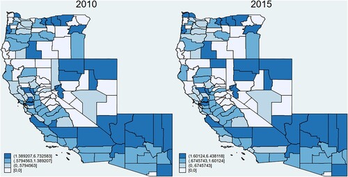
To illustrate our identification strategy based on contiguous states and counties, Figure 1 shows a map of the four states and the contiguous and non-contiguous counties in each state. Figure 2 reports the distribution of county-level Emissions per capita (ln) in 2010 and 2015. Apart from a few cases, the graphs do not suggest major changes in emissions at the county level. From the maps, it is clear that there is spatial clustering in the distribution of GHG emissions across the United States. Results based on Moran’s I test, available from the authors upon request, confirm this finding.

Figure 1. Counties in California and contiguous states: Oregon, Nevada and Arizona.

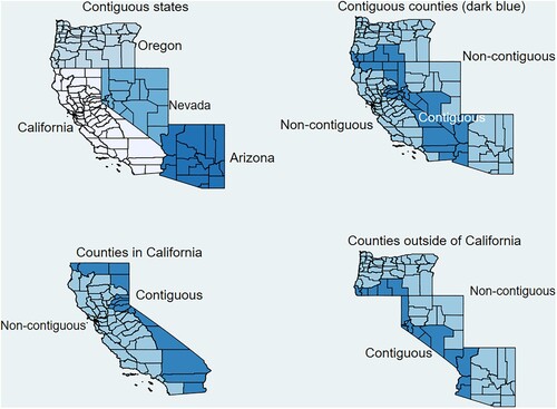
Figure 2. Emissions per capita (ln) in California and contiguous states: Oregon, Nevada and Arizona in 2010 and 2015.

3.2.2. Facility-level specifications

Our county-level regressions are based on aggregating facility-level emissions data, and this might result in loss of information. Additionally, since some counties do not have facilities that fall into the CATP rules, we might also have a limited number of counties in the treatment and control group. Such limitations might affect the precision of our estimates, especially in the regressions with only contiguous counties. For this reason, we run facility-level regressions to establish whether the total level of emissions at the facility level decreases in California relative to other states. Specifically, we estimate the following regression: (2) $Emission{s}_{it}={\alpha }_0+{\alpha }_1(Californi{a}_i\times Post{2013}_t)+{\nu }_i+{\lambda }_t+{\theta }_{it}$(2) where $Emission{s}_{it}$ is the natural logarithm of total emissions for facility i in year t. For these regressions, we cluster the standard errors at the county or at the facility level, depending on the specification. To improve the robustness of our analysis, not only do we build control groups on the basis of contiguous counties and states, but we also consider the geographical proximity between facilities in the two subsamples, measured using the formula introduced by Vincenty (1975). To be more precise, we calculate the distance across facilities and we focus on pairs of facilities that are nearest to each other, regardless of whether they belong to the treatment group or control group. Then, we keep only those cases for which the nearest facility is in the other subsample (either treatment group or control group). In other words, we are considering only those cases for which the facility in the control group is the nearest facility to the facility in the treatment group, among all facilities in the sample. We do this to avoid cases for which many facilities close to each other in the same subsample (treatment or control) are matched with the same facility across the Californian border (in the other subsample).

Table A2 in Appendix A in the supplemental data online, reports summary statistics for facility-level Emissions (ln) for the whole sample and for the subsample of facilities that are nearest to those in the treatment group. Table A2 also reports the summary statistics for the distance in kilometres for the facilities that are nearest to each other.

3.3. Preliminary analysis

Running DiD regressions is subject to the assumption that, in the absence of treatment, the trends in the variables under examination should be parallel. Recent contributions highlight that any difference in levels should also be discussed (Kahn-Lang & Lang, 2020). For this reason, we plot the trend of the main variables of interest over the sample period, considering different subsamples, and data at both the county and facility level. We report the results in Figure 3. The graphs show that the parallel trend assumption is likely to be satisfied in most cases. They also suggest that using contiguous counties – or the nearest facilities – as a control group results in better matching. In particular, for the county-level graphs the initial values of GDP per capita (ln) and Emissions per capita (ln) are closer when we consider contiguous counties, consistent with the claim that contiguous counties should be relatively more similar to each other (Huang, 2008) than counties far apart.

Figure 3. Parallel trend tests: (a) GDP per capita (ln) in California and all other states; (b) GDP per capita (ln) in contiguous counties in CA, OR, NV and AZ; (c) Emissions per capita (ln) in California and all other states; (d) Emissions per capita (ln) in contiguous counties in CA, OR, NV and AZ; (e) Emissions (ln) for facilities in California and facilities in other states; and (f) Emissions (ln) for facilities in CA and nearest facilities in contiguous states.

Note: CA, California; OR, Oregon; NV, Nevada; AZ, Arizona; GDP, gross domestic product.

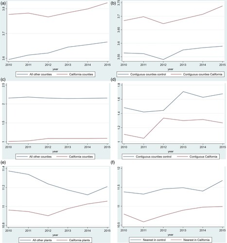
However, for contiguous counties, Emissions per capita (ln) in 2012 increased slightly more in California than in the contiguous states and flattened in 2013. Thus, there is some evidence of anticipation effects with respect to the introduction of the CATP in 2013. Other than this finding, the graphs seem to suggest that the CATP did not have a major effect on local economic growth, at least in the short run.

For the graphs based on facility-level data, in Figure 3e the pre-treatment average for Emissions (ln) for the facilities outside of California is monotonically decreasing, while the one for facilities in California is more stable and starts increasing in 2012. In Figure 3f, instead, the pre-treatment average for Emissions (ln) for the facilities outside of California does not follow a downward trend, and in fact the two lines appear to move more in sync than in Figure 3e.

Table 2 reports a similar analysis, using t-tests. To investigate whether the average growth rate of our main variables is similar for the treatment and control groups – as in Lemmon and Roberts (2010) – we run two-sample t-tests on the pre-treatment first-differences of the county-level variables GDP per capita (ln) and Emissions per capita (ln) using different matching strategies (panels A–C). In panel D, we show the results of t-tests on the first-differences of the facility-level variable Emissions (ln).

Table 2. T-tests on the average pre-treatment growth of the main variables.

(A) California versus other states	Observations	California = 0	California = 1	p-value
GDP per capita (ln), first difference – all counties	9255	0.0162	0.0001	0.0397
Emissions per capita (ln), first difference – all counties	3539	0.0108	0.0305	0.6015
GDP per capita (ln), first difference – contiguous counties	87	0.0061	0.0021	0.7740
Emissions per capita (ln), first difference – contiguous counties	26	−0.0196	0.0563	0.3020
(B) Border counties versus non-border counties in California		Non-border county	Border county
GDP per capita (ln), first difference	174	−0.0006	0.0021	0.7770
Emissions per capita (ln), first difference	82	0.0277	0.0563	0.7172
(C) Border counties versus non-border counties in Oregon, Nevada and Arizona		Non-border county	Border county
GDP per capita (ln), first difference	201	0.0155	0.0061	0.5062
Emissions per capita (ln), first difference	90	−0.0147	−0.0196	0.9134
(D) Facility level		California = 0	California = 1
Emissions (ln) – first difference – facilities in contiguous states	207	0.0303	0.0623	0.7107
Emissions (ln) – first difference – nearest facilities	143	−0.0581	0.0565	0.2828

Note: Presented are t-tests aimed at verifying statistical differences, during the pre-treatment period (2010–12), in the average growth of the main variables. Panel A reports t-tests for the pre-treatment period for counties in California versus counties in other states, separately for all counties (first two rows) and counties at the border between California and Oregon, California and Nevada, and California and Arizona (Contiguous Counties, third and fourth rows). Panel B reports t-tests for the same period for counties in California, where the two subsamples are counties at the border with Oregon, Nevada or Arizona, and counties that are not at the border. Panel C reports t-tests for the same period for counties in Oregon, Nevada and Arizona, where the two subsamples are counties at the border with California, and counties that are not at the border. Panel D reports t-tests for the same period using facility-level data, where the subsamples are facilities in California and facilities outside of California, separately for facilities in contiguous counties in California, Oregon, Nevada and Arizona (first row), and facilities that are nearest to those in California (second row). For panels A–C, we provide the statistics for the first-differences of GDP per capita (ln) and Emissions per capita (ln). For panel D, we use facility-level first-differenced Emissions (ln).

In panel A, we run the t-tests twice, first using all counties in California (treatment group, the dummy California is equal to 1) and other US states (control group, the dummy California is equal to 0), and then using only contiguous counties at the border between California and Oregon, California and Nevada, and California and Arizona. In panel B, we focus on counties in California, and the two subsamples are based on whether a county is at the border or not. In panel C, we do the same as in panel B for counties in Oregon, Nevada and Arizona. Finally, in panel D, we zoom in on facility-level t-tests, separately for facilities in border counties in California and adjacent states, and for facilities in the treatment and control group that are nearest to each other.

The results for the t-tests in panels A–D suggest that the parallel trend assumption is likely to be satisfied in most cases (p-values > 0.10), except for the test on the first differences of real GDP per capita using all counties, where p = 0.0397. In particular, local economic growth is, on average, lower in California than in other states. However, once we consider only contiguous counties, the p-value rises to around 0.77, suggesting that using only contiguous counties results in better matching between the treatment and control groups.

4. RESULTS

4.1. Main results

Table 3 reports the results of DiD regressions based on equation (1), for GDP per capita (ln) (panel A) and Emissions per capita (ln) (panel B).¹²

Table 3. Impact of Cap-and-Trade Program (CATP) on county-level gross domestic product (GDP) and total emissions per capita.

	(1)	(2)	(3)	(4)	(5)	(6)	(7)	(8)
	All states	Contiguous states	Contiguous counties	All states	All states	Contiguous states	Contiguous counties	All states
(A) GDP per capita (ln)
California × Post 2013 [A]	−0.0185**	0.0164	−0.0004	−0.0186*	0.0223*	0.0120	0.0110	0.0228*
	(−2.2976)	(0.9045)	(−0.0138)	(−1.9575)	(1.7798)	(0.4819)	(0.3207)	(1.8488)
California × Contiguous County × Post 2013 [B]				0.0183				0.0460*
				(0.6768)				(1.6723)
Contiguous County × Post 2013 [C]				−0.0183				−0.0211
				(−0.8337)				(−0.8789)
Controls	No	No	No	No	Yes	Yes	Yes	Yes
Observations	18,510	750	174	18,510	18,510	750	174	18,510
Counties	3085	125	29	3085	3085	125	29	3085
F-test [A + B + C = 0] – p-value	–	–	–	0.1581	–	–	–	0.0018
R^2	0.965	0.984	0.977	0.965	0.965	0.985	0.979	0.965
County fixed effects	Yes	Yes	Yes	Yes	Yes	Yes	Yes	Yes
Year fixed effects	Yes	Yes	Yes	Yes	Yes	Yes	Yes	Yes
(B) Emissions per capita (ln)
California × Post 2013 [A]	0.0536**	0.0071	−0.0226	0.0529*	0.0942***	0.0092	−0.2217*	0.0955***
	(1.9920)	(0.2237)	(−0.4356)	(1.7908)	(3.4310)	(0.2472)	(−1.7725)	(3.5280)
California × Contiguous County × Post 2013 [B]				−0.0788				−0.0642
				(−1.3831)				(−0.9795)
Contiguous County × Post 2013 [C]				0.0890**				0.0879**
				(2.4585)				(2.3618)
Controls	No	No	No	No	Yes	Yes	Yes	Yes
Observations	10,853	519	79	10,853	10,853	519	79	10,853
Counties	1905	88	14	1905	1905	88	14	1905
F-test [A + B + C = 0] – p-value	–	–	–	0.0727	–	–	–	0.0370
R^2	0.967	0.993	0.990	0.967	0.967	0.993	0.991	0.967
County fixed effects	Yes	Yes	Yes	Yes	Yes	Yes	Yes	Yes
Year fixed effects	Yes	Yes	Yes	Yes	Yes	Yes	Yes	Yes

Note: Reported are the results of DiD regressions on GDP per capita (ln) (panel A), and Emissions per capita (ln) (panel B). Specifications in columns (1), (4), (5) and (8) include observations from all US counties. Specifications in columns (2) and (6) include observations from all counties in California, Oregon, Nevada and Arizona. Specifications in columns (3) and (7) only include observations from counties located at the border between California and Oregon, California and Nevada, and California and Arizona. California is a dummy equal to 1 if the observation pertains to a county located in California, and 0 otherwise. Post 2013 is a dummy equal to 1 for the period 2013–15, and 0 before (i.e., 2010–12). Contiguous County is a time-invariant dummy equal to 1 for counties located at the border between California and Oregon, California and Nevada, California and Arizona, and 0 otherwise. columns (5)–(8) include as controls three additional variables: Non-manufacturing weight, which is equal to the percentage of county-level GDP associated with non-manufacturing sectors, and the interactions Non-manufacturing weight × Post 2013 and California × Non-manufacturing weight.

We run the DiD regressions on the whole sample of counties (column 1), on a subsample of counties in contiguous states (column 2), and on a subsample of counties at the border between California and adjacent states (column 3). Specification (4) is a triple DiD regression. We create a dummy, named Contiguous County, equal to 1 for counties at the border between California and contiguous states, and we interact it with Post 2013 and the interaction term California × Post 2013. We do not interact it with California because this interaction, like the dummy California, is subsumed by the county fixed effects.

In specifications (1)–(4), we do not consider the potential impact of cross-county heterogeneity in terms of industry structure. This is important because highly polluting sectors might represent a high share of GDP in certain counties but not others. For this reason, we create a variable, Non-manufacturing weight, which is equal to the percentage of county-level GDP associated with sectors other than manufacturing. We then include this variable in our regressions, and we also interact it with the dummies California and Post 2013, as well as their interaction, California × Post 2013. The results of these regressions are provided in columns (5)–(8). For the sake of space, we do not report the estimates for these controls.

The results in panel A suggest that the CATP reduced economic growth only when all counties are in the sample: the coefficient on California × Post 2013 is negative and significant at the 5% level in column (1),¹³ our baseline regression, and at the 10% level in column (4), which includes the triple interaction term California × Contiguous County × Post 2013. However, the coefficient on California × Post 2013 becomes positive and significant at the 10% level in columns (5) and (8) and statistically insignificant in columns (6) and (7).

The coefficient on California × Contiguous County × Post 2013 is insignificant in column (4) and significant at the 10% level in column (8). Table 3 also shows the results of F-tests for the sum of the coefficients on the interaction terms California × Post 2013 (denoted with an ‘A’), California × Contiguous County × Post 2013 (B), and Contiguous County × Post 2013 (C). These F-tests have p > 10% for specification (4), but p < 1% for specification (8). In the latter specification, the sum of the coefficients on A, B and C is positive. Thus, once we consider contiguous counties, the results for specification (8) suggest that there might have been an improvement in local economic growth as a result of the CATP in counties at the border.¹⁴ However, results in columns (3) and (7) – which derive from our preferred sample (as per preliminary parallel trend tests described in section 3.3) – reveal that the CATP does not affect GDP per capita (ln) in the short run.

For Emissions per capita (ln), in panel B, the coefficient on California × Post 2013 is positive and significant at the 5% level or better in columns (1), (5) and (8). In other specifications – including our preferred specifications (3) and (7) – the coefficient on this interaction term is statistically insignificant at the 5% level. Similar to the results reported in panel A, there is a positive effect on emissions per capita in contiguous counties in California, relative to other counties. The sum of the coefficients on A, B and C in column (8) is positive and statistically significant at the 5% level, although the coefficient on B is negative (but statistically insignificant). The coefficient on C, instead, is positive and significant at the 5% level in columns (4) and (8). Thus, these results suggest a positive impact of the CATP on counties at the border, regardless of whether they are in California or in adjacent states. Overall, these findings reveal the ineffectiveness, at least in the short term, of the CATP in curbing GHG emissions.

4.2. Facility-level regressions

In this section, we report the results of facility-level regressions run according to equation (2). The results in Table 4 confirm that the impact on emissions was either positive and significant at the 5% level (column 1) or insignificant, although in column (3) the coefficient on the interaction term turns negative and significant. However, the standard error of the coefficient on California × Post 2013 in column (3) is likely to be downward biased due to the county-level clustering with a low number of counties (14 counties in total). Once we use facility-level clustering (column 4), the coefficient becomes insignificant.

Table 4. Impact of the Cap-and-Trade Program (CATP): facility-level regressions.

Facility-level emissions (ln)	(1)	(2)	(3)	(4)	(5)	(6)
	All facilities	Contiguous states	Contiguous counties	Contiguous counties	Nearest facilities	Nearest facilities
California × Post 2013	0.1561***	−0.0278	−0.1982**	−0.1982	0.3471	0.3471
	(2.6288)	(−0.4116)	(−2.6742)	(−1.5490)	(1.2720)	(1.1162)
Observations	38,744	3944	662	662	461	461
Facilities	7154	711	121	121	84	84
Counties	1916	88	14	14	43	43
R^2	0.839	0.842	0.871	0.871	0.841	0.841
Facility fixed effects	Yes	Yes	Yes	Yes	Yes	Yes
Year fixed effects	Yes	Yes	Yes	Yes	Yes	Yes
Clustering	County level	County level	County level	Facility level	County level	Facility level

Note: Reported are the results of difference-in-differences (DiD) regressions run according to equation (2). Specifications in column (1) include observations from all US counties. Specifications in column (2) include observations from all counties in California, Oregon, Nevada and Arizona. Specifications in columns (3) and (4) only include observations from counties located at the border between California and other contiguous states. Specifications in columns (5) and (6) consider only the cases for which the facilities in the treatment and control group are the nearest ones to each other in our sample.

Overall, the findings in this section suggest very little (if any) evidence of a reduction in facility-level emissions, regardless of the matching procedure employed.

5. THE MECHANISM: ALLOWING FOR OWNER-LEVEL DECISIONS

5.1. Leakage versus portfolio rebalancing

In addition to facility-level data, we also exploit information on the parent organisations owning the facilities. An organisation in our database might own more than one facility, and each facility could have more than one owner. Thus, time-invariant components at the parent level might play a role because the organisations owning the facilities might make decisions on the level of emissions, on the basis of the location of the facilities in their portfolio. For this reason, we run another set of regressions where the focus is on the organisations owning the facilities.

It is important to note that we use the name ‘organisations’ instead of ‘firms’ because we employ the whole database of facilities’ owners, and many of these organisations are not firms. For example, the facilities could be owned by local authorities (e.g., City of Chattanooga, Tennessee) or universities (e.g., University of California San Diego). Our dataset hence comprises more than 7000 facilities and about 3700 parent organisations. Using the full dataset on GHG emissions enables us to mitigate such selection-bias concerns, ultimately leading to a more precise and comprehensive analysis of the phenomenon under investigation.

The facility–parent matched data gives us the opportunity to test if owners of facilities in both California and other states exploited the incompleteness of the regulation to transfer emissions to other states, resulting in leakage. Evidence of cross-country leakage exists with respect to international climate policies such as the Kyoto protocol (Aichele & Felbermayr, 2015). Existing empirical literature finds that this is indeed the case (Bartram et al., 2022), but these findings are based on a subsample of listed firms, and exclude the utilities sector (in addition to the financial sector), which is one of the most polluting industries. Recent literature on carbon pricing includes utility stocks because of this reason (Bolton & Kacperczyk, 2021).

If leakage occurs because of such a transfer of emissions outside of California, we should expect a positive impact of the CATP on the emissions of organisations with facilities both inside and outside of California relative to other organisations.

We also test the potential impact on market structure. In particular, we test if the CATP results in changes in market concentration for emission-dependent organisations. In fact, rather than moving emissions outside of California, parent organisations with facilities in both California and other states might simply reduce their ownership stake in facilities in California to consolidate their market share (in terms of GHG emissions) outside of California. In other words, rather than moving emissions, parent organisations might change the composition of facilities in their portfolio. For this reason, we measure the average county-level market share in emissions for each parent organisation (we call this ‘parent-level market share’). Then, we test if, following the CATP, parent organisations rebalance their facilities portfolios, by selling or buying facilities in California and other states. We also measure the impact in terms of overall concentration, using the Herfindahl–Hirschman index (HHI). Therefore, we measure the average market share and HHI using facility–parent matched data, considering the market share of the counties where the owners have facilities. This set-up aims to establish whether parent organisations with facilities in California adjust their ownership shares of facilities in their portfolios, resulting in different levels of market concentration in emissions. In particular, using facility–parent level data allows us to exploit both the location of the facility (necessary for our DiD set-up based on facilities’ location) and parent-level fixed effects. For this reason, instead of collapsing the observations at the parent-level, which would eliminate the information on the location of the facilities for multi-facilities organisations, we run the regressions at the facility–parent level.

5.2. Methodology and data: facility–parent specifications

To test whether parent organisations transfer emissions outside of California, we create a variable, Multiple, which is equal to 1 if, in a given year, an organisation has facilities both in California and in other states, and 0 otherwise. Since this variable can vary over time, we can include it in the regressions with parent and year fixed effects. We then interact this variable with the interaction California × Post 2013, as follows: (3) $\begin{array}{rl}{y}_{ipt}=& {\alpha }_0+{\alpha }_1(Californi{a}_{ip}\times Post{2013}_t)+{\alpha }_{2}Multipl{e}_{pt}\\ & +{\alpha }_3(Californi{a}_{ip}\times Multipl{e}_{pt}\times Post{2013}_t)\\ & +{\varphi }_p+{\lambda }_t+{\delta }_{ipt}.\end{array}$(3) where, as before, the subscript $i$ denotes the facility, while $p$ denotes the parent organisation(s) owning the facility, and ${\varphi }_p$ are parent fixed effects. For example, the dummy variable $Californi{a}_{ip}$ denotes facilities in California owned by parent $p$.

We also run the baseline regressions with California × Post 2013 only for observations for which Multiple is equal to 1. This enables us to investigate whether the findings for our facility–parent level regressions are driven by systematic differences between facilities owned by organisations with facilities both in California and other states, and facilities owned by other organisations.

To improve robustness, we home in on facilities outside of California, and run the regression: (4) $y_{ipt}={\alpha }_0+{\alpha }_{1}Multipl{e}_{pt}+{\alpha }_2(Multipl{e}_{pt}\times Post{2013}_t)+{\varphi }_p+{\psi }_{st}+{\delta }_{ipt}$(4) In the above equation, ${\psi }_{st}$ are industry-year fixed effects, where the industry is identified by the facility-level North American Industry Classification System (NAICS) code. For robustness, we also run the same regression after replacing ${\psi }_{st}$ with year fixed effects (i.e., without interacting the latter with NAICS fixed effects).

We also specifically test for the impact on the proportion of emissions from facilities outside of California for parent organisations that operate facilities both in and out of California (i.e., Multiple = 1). We call the ratio of emissions from counties outside of California divided by the total emissions Emissions ratio, and we run the following regression: (5) $Emissionsrati{o}_{ipt}={\alpha }_0+{\alpha }_1(Californi{a}_{ip}\times Post{2013}_t)+{\varphi }_p+{\lambda }_t+{\theta }_{ipt}$(5) As explained in section 5.1, we also examine changes in the concentration of GHG emissions of different parent organisations. First, we calculate, for each parent, the average share of emissions produced in each county and year. Larger market shares of a parent in a given county indicate that the facilities owned by that organisation emit a larger portion of GHG in that county. For each parent–facility combination, we take the average market share of the parent organisation in all counties where it owns facilities. Moreover, we also calculate the HHI in emissions, on the basis of the computed market shares. Therefore, a high (low) parent-level market share or HHI suggests that the organisation owns facilities in counties with a relatively more concentrated market structure.¹⁵

We then estimate the following regressions, using county, parent, and year fixed effects: (6a) $Shar{e}_{ipct}={\alpha }_0+{\alpha }_1(Californi{a}_i\times Post{2013}_t)+{\gamma }_c+{\varphi }_p+{\lambda }_t+{\theta }_{ipct}$(6a) (6b) $HH{I}_{ipct}={\alpha }_0+{\alpha }_1(Californi{a}_i\times Post{2013}_t)+{\gamma }_c+{\varphi }_p+{\lambda }_t+{\theta }_{ipct}$(6b) We run regressions (6a) and (6b) using all counties, only counties in California, Oregon, Nevada and Arizona, and only contiguous counties at the border between California and contiguous states (Oregon, Nevada and Arizona). We cluster the standard errors at the parent level. We also use propensity score matching (PSM) techniques in the regressions for equations (6a) and (6b).

5.3. Results: facility–parent specifications

Table 5 reports the results of regressions run according to equations (3) and (4). Since the same facility can belong to more than one parent organisation, in some instances we have more observations for the facility–parent regressions than for the corresponding facility-level regressions. To allow for serial correlation, we cluster the standard errors at the county or parent-level, depending on the specification.

Table 5. The mechanism: parent-level regressions.

	(1)	(2)	(3)	(4)	(5)	(6)	(7)
	Emissions (ln)	Emissions (ln)	Emissions (ln)	Emissions (ln)	Emissions (ln)	Emissions ratio	Emissions ratio
	All parents	All parents	Multiple = 1	All parents	All parents	Multiple = 1	Multiple = 1
California × Post 2013	−0.0675	−0.0643	−0.1645			−0.0022	−0.0011
	(−0.6168)	(−0.4588)	(−1.1733)			(−0.9645)	(−0.2537)
California × Multiple × Post 2013	−0.0603	−0.0489
	(−0.3906)	(−0.2458)
Multiple × Post 2013				−0.0242	−0.0287
				(−0.4229)	(−0.5359)
Multiple	0.0810	0.0945		0.0200	0.0608
	(0.9660)	(1.1873)		(0.2972)	(0.8319)
Observations	46,532	43,376	8576	43,004	43,377	8576	8056
Parents	3695	3521	175	3397	3435	175	174
R^2	0.426	0.435	0.231	0.482	0.431	0.908	0.910
Parent fixed effects	Yes	Yes	Yes	Yes	Yes	Yes	Yes
Year fixed effects	Yes	Yes	Yes	No	Yes	Yes	Yes
Industry-year fixed effects	No	No	No	Yes	No	No	No
Clustering	Parent level	County level	Parent level	Parent level	Parent level	Parent level	County level

Note: Reported are the results of facility-level regressions run according to equation (3), columns (1)–(3), equation (4), columns (4) and (5), and equation (5), columns (6) and (7). ‘Multiple = 1’ refers to cases for which a parent organisation has facilities both in and out of California. ‘Emissions (ln)’ is the natural logarithm of facility-level emissions. ‘Emissions ratio’ is the ratio of emissions coming from facilities outside California divided by the total amount of emissions from all facilities for parent organisations for which Multiple = 1.

The results for equations (3) and (4) suggest that the impact of the CATP is insignificant. In particular, the coefficients on the interaction terms California × Post 2013 tend to be insignificant, as are those on the triple interaction term California × Multiple × Post 2013. Thus, the results in Table 5 do not indicate that parent organisations tend to shift emissions outside of California.

Finally, the results of the tests regarding concentration in emissions are reported in Table 6. Even in this case, we observe starkly different results depending on the level of the matching procedure. In particular, the regression using all facilities suggests a positive impact (significant at the 5% level) of the CATP on the average market share and HHI in emissions (column 1), in both panels. On the other hand, the coefficient on California × Post 2013 for a subsample considering only facilities in California and contiguous states – column (2) – is statistically insignificant for both the regressions on the average market share and those on the HHI. Lastly, when we include only facilities in contiguous counties – column (3) – the coefficient turns negative and statistically significant at the 10% level for the regression on the average market share and at the 1% level for the one on the HHI.

Table 6. Impact of the Cap-and-Trade Program (CATP) on the average parent-level market share and Herfindahl–Hirschman index (HHI).

	(1)	(2)	(3)	(4)
	All facilities	Contiguous states	Contiguous counties	Contiguous counties (PSM)
(A) Market share
California × Post 2013	0.0082**	−0.0018	−0.0357*	−0.0369**
	(2.0621)	(−0.2104)	(−1.8153)	(−2.0018)
Observations	43,360	4365	704	354
Parents	3521	536	112	65
Counties	1908	88	14	12
^R^2	0.936	0.941	0.951	0.944
County fixed effects	Yes	Yes	Yes	Yes
Parent fixed effects	Yes	Yes	Yes	Yes
Year fixed effects	Yes	Yes	Yes	Yes
Clustering	Parent level	Parent level	Parent level	Parent level
(B) HHI
California × Post 2013	3.9158**	−5.5482	−37.7853***	−40.8361***
	(2.2252)	(−1.2194)	(−3.6588)	(−3.7492)
Observations	43,360	4365	704	354
Parents	3521	536	112	65
Counties	1908	88	14	12
R^2	0.929	0.897	0.886	0.865
County fixed effects	Yes	Yes	Yes	Yes
Parent fixed effects	Yes	Yes	Yes	Yes
Year fixed effects	Yes	Yes	Yes	Yes
Clustering	Parent level	Parent level	Parent level	Parent level

Note: Reported are the results of facility-parent level regressions run on the parent-level average market share and HHI calculated following equations (6a), panel A, and (6b), panel B, respectively. Specifications in column (4) are run on matched samples.

In column (4), we report results of regressions obtained via a PSM approach – using only facilities in contiguous counties – where we match facilities on the basis of pre-treatment growth in county-level emissions, pre-treatment growth in parent-level average market share and HHI for emissions, location of the facility (longitude and latitude), percentage of facility-level GHG emissions consisting of $\mathrm{C}{\mathrm{O}}_2$ emissions, the dummy Multiple, and the three-digit NAICS of the facility. The propensity score was unbalanced before matching, but it becomes balanced afterwards. Before matching, Rubin’s B is equal to 306.7, which is much higher than 25, and Rubin’s R is 3.54 (well above the upper critical value of 2). After the matching, using a calliper equal to 0.0001, the value for Rubin’s B becomes zero, and the one for Rubin’s R becomes 1 (within the critical values of 0.5 and 2). Then, we exclude the observations outside of the common support, and we run the regressions on contiguous counties again. The results for column (4) remain consistent with those in column (3) for both panels A and B. In particular, the coefficient on California × Post 2013 for the regression on the average market share, in panel A, becomes significant at the 5% level.¹⁶

Overall, these findings reveal that, similar to the results in previous sections, the matching procedure bears major implications on our inferences. The results using our preferred specification – which includes only counties at the border – indicate that the CATP decreases the HHI for facilities in California, relative to facilities in adjacent states. Since the results in Table 5 do not suggest a transfer in emissions from California to other states, the observed effects on the HHI must be related to changes in the ownership of the facilities. Moreover, the negative coefficient on California × Post 2013 suggests that the CATP reduces the degree of market concentration in the counties at the border in California, relative to adjacent counties. This implies that organisations in California with large HHIs reduce their ownership stakes with respect to other organisations with a lower HHI.

6. POLICY IMPLICATIONS

Several regional policy implications can be drawn from our study. From a theoretical perspective, cap-and-trade systems could be more efficient than systems based on rewards and sanctions, as they may result in a reallocation of incentives whereby greener organisations act as emission-permit suppliers, while emission-dependent organisations (such as energy companies) become buyers of emission permits, provided that they are likely to exceed their allocated quotas (Du et al., 2015). Despite such a reallocation of incentives, assuming that the allowances are binding, the overall volume of emissions at the regional level – considering both emission-dependent and emission-supplying organisations – should decrease. Importantly, such a reduction in emissions could lead to a reduction in local economic growth. However, lower emissions do not necessarily lead to lower economic growth if firms shift their focus from polluting sectors to green sectors, a phenomenon known as ‘decoupling’ (Granados & Spash, 2019). We fail to provide robust evidence that the Californian CATP led to a decrease in emissions and GDP growth. From a regional policymaking perspective, such a lack of evidence of a reduction of emissions in the short term is undoubtedly a problem, although it is reassuring to observe that the CATP did not worsen regional economic growth.

Cap-and-trade regulations might fail to reduce emissions at the regional level because of a poorly designed allowance-allocation system (Lange & Maniloff, 2021). Even in the presence of a regulatory floor for the price of allowances, if the cap is not low enough relative to business-as-usual emissions, the impact on local emissions – relative to unregulated regions – might be negligible. Therefore, when choosing the cap, authorities must consider uncertainty in future demand for emissions and the need to find a politically acceptable price for allowances (Borenstein et al., 2019).

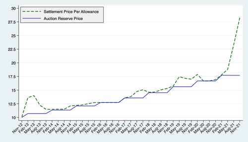
National governments may gain from decentralised policymaking initiatives on environmental matters (Heim et al., 2022), as long as potential stakeholders do not interfere in the design of such measures. As mentioned in section 2, lobbying activities from emitters can affect the political process related to climate regulation, leading to a non-binding cap (Adam, 2011). Although we do not test for regulatory capture directly, our results might be explained by a weak auction demand for allowances, especially in the first three years of the CATP (Busch, 2017). These claims are supported by the data in Figure 4, which reports auction prices for the CATP from November 2012 to November 2021. The graph shows that settlement prices for allowances have mostly been close to the floor represented by the auction reserve price, except for a significant spike recorded in the last two auctions of 2021. In particular, the price of allowances was in the range US$10–14 in the period from 2013 to 2015, while in 2021 the price exceeded US$27.

Figure 4. Auction prices.

Our results also bear other major regional policy implications. Specifically, our analyses of the mechanism underlying our main findings rule out the possibility of emissions leakage in the form of transfer of emissions from facilities in regulated regions to facilities in unregulated regions. Nonetheless, we are the first to uncover a novel form of regulatory arbitrage, for multi-state organisations, based on adjusting their ownership shares of facilities in different states. Intuitively, this behaviour enables multi-state organisations to decrease their individual accountability for the emissions in regulated states, while keeping the facilities’ overall contribution to emissions at the aggregate level unchanged. This conduct changes the ownership concentration of emissions rather than the level of emissions, and it might be argued that such a behaviour does not carry major environmental consequences at the regional level. However, facility-level changes in ownership might affect the strategic importance of that facility to its ultimate owner, leading to technological and other operational shifts that might influence the local economy and labour market of that region.

The enforcement of a regional CATP might dissuade existing companies from creating new facilities in the regions affected by such policy. Moreover, companies might plan to open new facilities in territories exempted from the CATP or similar programmes. Likewise, companies might decide to adjust the ownership share of their facilities, as we observe from our analyses. Firms can reduce their stakes in facilities subject to the CATP and purchase – or increase their ownership share in – facilities in other states. This could be done relatively quickly and would not require new ad-hoc investments.

To conclude, our results highlight the importance of a regional approach when evaluating climate policies. In particular, the unit of analysis (county level) and spatial distance between the control and treatment units is crucial for the interpretation of the results. For this reason, our results support recent calls for an integrated approach by national and regional policymakers (Heim et al., 2022) when designing cap-and-trade policies and evaluating their effects. Moreover, since many facilities included in our analysis might be part of global value chains, our results also suggest that regional cap-and-trade systems should be seen as components of modular interventions – where ‘local’ and ‘global’ actions are integrated (Crescenzi & Iammarino, 2017) – rather than stand-alone policies.

7. CONCLUSIONS

This paper contributes to the policy debate regarding the effectiveness of climate policy regulations and their real effects. Our findings reveal unintended consequences of these regulations that only a regional perspective can bring to light.

We are the first to show that the California CATP did not result in lower county-level GHG emissions per capita, nor did it impair local economic growth (GDP per capita). Moreover, by exploiting facility-level data and information on the parent organisations owning the facilities, we document that parent organisations owning facilities in California and other states rebalanced their ownership portfolio, leading to changes in county-level market shares and HHI in emissions. On the other hand, we do not find evidence of leakage in the form of a transfer of emissions from facilities in California to facilities in other states.

From a regional perspective, our empirical investigation is important for the following reasons. First, by comparing a variety of matching strategies, our findings suggest that using a suboptimal control group might have severe consequences on inferences and, ultimately, the evaluation of the impact of climate policies at the regional level. Using all US counties, we obtain counter-intuitive results: county-level economic growth falls following the implementation of the CATP, despite an increase in county-level emissions. Second, our study highlights the need to monitor the behaviour of parent organisations, not only in terms of facility-level emissions, but also with respect to their overall portfolio of facilities. Such a holistic perspective is essential to understand how regional regulations might influence the incentives and industrial strategies of parent organisations and, in turn, their repercussions on local socio-economic conditions.

Our study allows us to provide important lessons for regional policymakers. While each region has its peculiarities, and thus drawing inferences for other regions necessarily requires adjustments to local specificities, our results suggest that regional cap-and-trade programmes might be successful in countries other than the United States as long as the cap is indeed binding. Ultimately, the outcome of this type of programmes depends on the degree to which emitters lobby for a higher cap. Regional initiatives might be more successful in countries where lobbying and regulatory capture are less likely to occur. There is a trade-off between a hard stance against lobbying, which might lead to relocation of factories in other regions, and a more sympathetic behaviour towards emitters, which might undermine the societal goal to curb emissions (Patnaik, 2019).

We are also aware that our study presents two limitations. First, free emission allowances were offered to some organisations in an attempt to reduce leakage. To better understand whether such measures have been effective, we would need detailed micro-level information on the facilities that benefited from such allowances. This information, though, is only available at the industry level rather than the facility level. Second, our analysis does not provide direct evidence of regulatory capture due to personal connections between local politicians and facility owners or lobbying activities by emitters. This type of analysis is hindered by data-availability constraints.

We believe that future research could address the data limitations above to further investigate the potential causes of ineffectiveness of cap-and-trade systems at the regional level. This is important because of the potential regional nature of spillovers in both emissions and economic growth. Our paper constitutes a first step in this direction, but our analysis is limited to the CATP in California.

ACKNOWLEDGEMENTS

We thank Professor Phil Tomlinson (editor) and two referees for their helpful suggestions. We are also grateful to Valeriya Dinger, Amine Ouazad and the participants at the IFABS 2022 conference (Naples, Italy) and the 2022 World Finance & Banking Symposium (Miami, FL, USA) for their comments on previous versions of the paper.

DISCLOSURE STATEMENT

No potential conflict of interest was reported by the authors.

Notes

1. See https://eu.azcentral.com/story/news/local/arizona-environment/2020/09/25/arizona-was-once-climate-policy-leader-in-west-what-happened/5841376002/. For more information on the Western Climate Initiative, see https://wci-inc.org/.

2. Nevada introduced targets in 2019, much later than our sample period (2010–15).

3. Oregon introduced statutory targets in 2007 (https://www.c2es.org/content/state-climate-policy/). However, the Oregon Department of Environment Quality (2015) admits that ‘Statewide emissions declined from 2007 through 2012 but recent data do not indicate a continuation of that downward trend’. Since 2012 belongs to our pre-treatment period (i.e., before the CATP), it is likely that the statutory target did not affect the post-treatment period.

4. Similar to Cermeño (2019), we scale our county-level dependent variables by the number of inhabitants to allow for size effects. For consistency, GHG emissions are also on a per capita basis in our county-level regressions. Irrespective of this scaling adjustment, unreported tests reveal that our results are virtually the same if we do not scale our variables by a county’s population. Moreover, for robustness, we also use facility-level emissions in our empirical analysis.

5. We acknowledge that local emissions contribute to the broader phenomenon of global warming (see, inter alia, Avci et al., 2015). Therefore, using counties contiguous to California as the main ‘competitors’ (in terms of CATP-free regions) does not capture the potential relocation of polluting facilities away from the neighbouring territories, apart from the decrease in emissions (if any) in California. Nonetheless, we believe that using contiguous counties is important because of the local dimension of emissions. Such a dimension allows us to capture the impact of important political pressures at the local level (e.g., lobbying from producers), which might be neglected by analyses using coarser units of analysis. In fact, the local dimension of the impact of the CATP has recently drawn attention from the media because facilities tend to be in low-income areas (https://www.latimes.com/california/story/2022-03-22/what-has-california-cap-and-trade-accomplished). Finally, although we focus on US counties, the implications of our results can be extended to regional policies in other countries because the mechanism through which regional cap-and-trade regulations operate are similar, although their details might differ (i.e., allocation and pricing rules of allowances).

6. Generally, the term ‘leakage’ refers to an increase in emission production of unregulated emitters as a result of incomplete environmental regulation (Fowlie, 2009).

7. Critics have also argued that cap-and-trade systems perpetuate the interest of multinationals and developed nations (Böhm et al., 2012; Newell & Paterson, 2010).

8. See https://apps.bea.gov/regional/downloadzip.cfm/.

9. See https://www.epa.gov/ghgreporting/archive-ghg-reporting-program-data-sets/.

10. We are aware that implementing the CATP might affect firms’ choices regarding facility refresh/renewal or greenfield investment. For example, it is plausible that firms do not shut down profitable plants because of the CATP, but they may build a new plant elsewhere upon renewal – a process that may take decades (e.g., for the steel and refinery industries). For this reason, it might take time for some of the effects of the CATP to unfold. Hence, with our short-term focus, we may not fully capture the outcomes of changes to plant life cycles. However, a long-term analysis would inevitably increase the chance of confounding events within the sample period, resulting in incorrect inferences. Ultimately, there is a trade-off between the reliability of the econometric approach and the extent to which we observe the effect of long-term firm policy decisions. Considering three years before and after the CATP allows us to strike a balance between these two factors.

11. As reported in section 5.1, there can be more than one owner for a facility.

12. As per note 3, the results are virtually the same if we do not adjust our variables to account for a county’s size (as proxied by its population).

13. The coefficient on California × Post 2013 in column (1) is $-0.0185$, suggesting an impact on real GDP per capita (not in logs) equal to: $100\times [exp(-0.0185)-1]=-1.833\text{\%}$. The average real GDP per capita in natural logarithms is 3.6353 (Table 1). Thus, the average real GDP per capita in thousands of US dollars is $exp(3.6353)=37.9$. Therefore, a reduction by $-1.833\text{\%}$ of average GDP per capita equals $-1.833\text{\%}\times 37,900=-\mathrm{\$}694.95$.

14. The coefficient on the triple interaction term California × Post 2013 × Non-manufacturing weight’ is negative and significant at the 1% level in specifications (5) and (8) in the regressions on GDP per capita (ln), and always insignificant at the 5% level in those on Emissions per capita (ln).

15. The parent-level HHI is similar to the bank-level HHI employed, for example, by Schaffer and Segev (2022) as a proxy for market concentration.

16. The response to the CATP might differ for owners with substantial amounts of immobile assets. For this reason, we also run these regressions again, considering only those facilities owned by universities, cities (or municipalities or county authorities) and utilities. We identify the type of owners based on the NAICS of the facility, but also the name of the owner (e.g., ‘University of Texas Austin’). For the aforementioned subsample of facilities, we estimate regressions based on the same set of specifications as in Table 6. The results, available from the authors upon request, are remarkably similar to those reported in Table 6.

REFERENCES

- Acuto, M. (2016). Give cities a seat at the top table. Nature, 537(7622), 611–613. https://doi.org/10.1038/537611a
- Adam, D. (2011). Money not the problem in US climate debate. Nature. https://doi.org/10.1038/news.2011.248
- Aichele, R., & Felbermayr, G. (2015). Kyoto and carbon leakage: An empirical analysis of the carbon content of bilateral trade. The Review of Economics and Statistics, 97(1), 104–115. https://doi.org/10.1162/REST_a_00438
- Avci, B., Girotra, K., & Netessine, S. (2014). Electric vehicles with a battery switching station: Adoption and environmental impact. Management Science, 61(4), 772–794. https://doi.org/10.1287/mnsc.2014.1916
- Aysheshim, K., Hinson, J. R., & Panek, S. D. (2020). A primer on local area gross domestic product methodology. Survey of Current Business, 100(3), 1–13. https://apps.bea.gov/scb/issues/2020/03-march/0320-county-level-gdp.htm
- Baldwin, J. G., & Wing, I. S. (2013). The spatiotemporal evolution of US carbon dioxide emissions: Stylized facts and implications for climate policy. Journal of Regional Science, 53(4), 672–689. https://doi.org/10.1111/jors.12028
- Bartram, S. M., Hou, K., & Kim, S. (2022). Real effects of climate policy: Financial constraints and spillovers. Journal of Financial Economics, 143(2), 668–696. https://doi.org/10.1016/j.jfineco.2021.06.015
- Biswas, S., Chakraborty, I., & Hai, R. (2017). Income inequality, tax policy, and economic growth. The Economic Journal, 127(601), 688–727. https://doi.org/10.1111/ecoj.12485
- Böhm, S., Misoczky, M. C., & Moog, S. (2012). Greening capitalism? A Marxist critique of carbon markets. Organization Studies, 33(11), 1617–1638. https://doi.org/10.1177/0170840612463326
- Bolton, P., & Kacperczyk, M. (2021). Do investors care about carbon risk? Journal of Financial Economics, 142(2), 517–549. https://doi.org/10.1016/j.jfineco.2021.05.008
- Bonnett, N. L., & Birchall, S. J. (2022). The influence of regional strategic policy on municipal climate adaptation planning. Regional Studies, 57(1), 141–152. https://doi.org/10.1080/00343404.2022.2049224
- Borck, R. (2016). Will skyscrapers save the planet? Building height limits and urban greenhouse gas emissions. Regional Science and Urban Economics, 58, 13–25. https://doi.org/10.1016/j.regsciurbeco.2016.01.004
- Borenstein, S., Bushnell, J., Wolak, F. A., & Zaragoza-Watkins, M. (2019). Expecting the unexpected: Emissions uncertainty and environmental market design. American Economic Review, 109(11), 3953–3977. https://doi.org/10.1257/aer.20161218
- Busch, C. (2017). Recalibrating California’s Cap-and-Trade Program to account for oversupply. Energy Innovation LLC.
- Camagni, R., & Capello, R. (2013). Regional competitiveness and territorial capital: A conceptual approach and empirical evidence from the European Union. Regional Studies, 47(9), 1383–1402. https://doi.org/10.1080/00343404.2012.681640
- Cermeño, A. L. (2019). Do universities generate spatial spillovers? Evidence from US counties between 1930 and 2010. Journal of Economic Geography, 19(6), 1173–1210. https://doi.org/10.1093/jeg/lby055
- Cojoianu, T. F., Ascui, F., Clark, G. L., Hoepner, A. G., & Wójcik, D. (2021). Does the fossil fuel divestment movement impact new oil and gas fundraising? Journal of Economic Geography, 21(1), 141–164. https://doi.org/10.1093/jeg/lbaa027
- Crescenzi, R., & Iammarino, S. (2017). Global investments and regional development trajectories: The missing links. Regional Studies, 51(1), 97–115. https://doi.org/10.1080/00343404.2016.1262016
- Cui, C. X., Hanley, N., McGregor, P., Swales, K., Turner, K., & Yin, Y. P. (2017). Impacts of regional productivity growth, decoupling and pollution leakage. Regional Studies, 51(9), 1324–1335. https://doi.org/10.1080/00343404.2016.1167865
- Deutz, P., & Gibbs, D. (2008). Industrial ecology and regional development: Eco-industrial development as cluster policy. Regional Studies, 42(10), 1313–1328. https://doi.org/10.1080/00343400802195121
- Du, S., Ma, F., Fu, Z., Zhu, L., & Zhang, J. (2015). Game-theoretic analysis for an emission-dependent supply chain in a ‘cap-and-trade’ system. Annals of Operations Research, 228(1), 135–149. https://doi.org/10.1007/s10479-011-0964-6
- Egger, P. H., & Lassmann, A. (2015). The causal impact of common native language on international trade: Evidence from a spatial regression discontinuity design. The Economic Journal, 125(584), 699–745. https://doi.org/10.1111/ecoj.12253
- Feyrer, J., Mansur, E., & Sacerdote, B. (2020). Geographic dispersion of economic shocks: Evidence from the fracking revolution: Reply. American Economic Review, 110(6), 1914–1920. https://doi.org/10.1257/aer.20190448
- Feyrer, J., Mansur, E. T., & Sacerdote, B. (2017). Geographic dispersion of economic shocks: Evidence from the fracking revolution. American Economic Review, 107(4), 1313–1334. https://doi.org/10.1257/aer.20151326
- Fowlie, M. L. (2009). Incomplete environmental regulation, imperfect competition, and emissions leakage. American Economic Journal: Economic Policy, 1(2), 72–112. https://doi.org/10.1257/pol.1.2.72
- Gibbs, D., Deutz, P., & Proctor, A. (2005). Industrial ecology and eco-industrial development: A potential paradigm for local and regional development? Regional Studies, 39(2), 171–183. https://doi.org/10.1080/003434005200059959
- Gibbs, D., & Jensen, P. D. (2022). Chasing after the wind? Green economy strategies, path creation and transitions in the offshore wind industry. Regional Studies, 56(1), 1671–1682. https://doi.org/10.1080/00343404.2021.2000958
- Gibbs, D., & O’Neill, K. (2017). Future green economies and regional development: A research agenda. Regional Studies, 51(1), 161–173. https://doi.org/10.1080/00343404.2016.1255719
- Granados, J. A. T., & Spash, C. L. (2019). Policies to reduce CO2 emissions: Fallacies and evidence from the United States and California. Environmental Science & Policy, 94, 262–266. https://doi.org/10.1016/j.envsci.2019.01.007
- Heim, I., Crowley-Vigneau, A., & Kalyuzhnova, Y. (2022). Environmental and socio-economic policies in oil and gas regions: Triple bottom line approach. Regional Studies, 57(1), 181–195. https://doi.org/10.1080/00343404.2022.2056589
- Huang, R. R. (2008). Evaluating the real effect of bank branching deregulation: Comparing contiguous counties across US state borders. Journal of Financial Economics, 87(3), 678–705. https://doi.org/10.1016/j.jfineco.2007.01.004
- James, A. G., & Smith, B. (2020). Geographic dispersion of economic shocks: Evidence from the fracking revolution: Comment. American Economic Review, 110(6), 1905–1913. https://doi.org/10.1257/aer.20180888
- Jones, S. (2019). City governments measuring their response to climate change. Regional Studies, 53(1), 146–155. https://doi.org/10.1080/00343404.2018.1463517
- Kahn-Lang, A., & Lang, K. (2020). The promise and pitfalls of differences-in-differences: Reflections on 16 and pregnant and other applications. Journal of Business & Economic Statistics, 38(3), 613–620. https://doi.org/10.1080/07350015.2018.1546591
- Knight, E. R. (2011). The economic geography of European carbon market trading. Journal of Economic Geography, 11(5), 817–841. https://doi.org/10.1093/jeg/lbq027
- Lange, I., & Maniloff, P. (2021). Updating allowance allocations in cap-and-trade: Evidence from the NOx budget program. Journal of Environmental Economics and Management, 105, 102380. https://doi.org/10.1016/j.jeem.2020.102380
- Lemmon, M., & Roberts, M. R. (2010). The response of corporate financing and investment to changes in the supply of credit. Journal of Financial and Quantitative Analysis, 45(3), 555–587. https://doi.org/10.1017/S0022109010000256
- Liu, C., & Williams, N. (2019). State-level implications of federal tax policies. Journal of Monetary Economics, 105, 74–90. https://doi.org/10.1016/j.jmoneco.2019.04.005
- Newell, P., & Paterson, M. (2010). Climate capitalism: Global warming and the transformation of the global economy. Cambridge University Press.
- Oregon Department of Environment Quality. (2015). Oregon’s greenhouse gas emissions through 2015: An assessment of Oregon’s sector-based and consumption-based greenhouse gas emissions (May). https://www.oregon.gov/deq/FilterDocs/OregonGHGreport.pdf
- Patnaik, S. (2019). A cross-country study of collective political strategy: Greenhouse gas regulations in the European Union. Journal of International Business Studies, 50(7), 1130–1155. https://doi.org/10.1057/s41267-019-00238-4
- Sancino, A., Stafford, M., Braga, A., & Budd, L. (2022). What can city leaders do for climate change? Insights from the C40 cities climate leadership group network. Regional Studies, 56(7), 1224–1233. https://doi.org/10.1080/00343404.2021.2005244
- Schaffer, M., & Segev, N. (2022). The deposits channel revisited. Journal of Applied Econometrics, 37(2), 450–458. https://doi.org/10.1002/jae.2869
- Turok, I., Bailey, D., Clark, J., Du, J., Fratesi, U., Fritsch, M., Harrison, J., Kemeny, T., Kogler, D., Lagendijk, A., Mickiewicz, T., Miguelez, E., Usai, S., & Wishlade, F. (2017). Global reversal, regional revival? Regional Studies, 51(1), 1–8. https://doi.org/10.1080/00343404.2016.1255720
- Vincenty, T. (1975). Direct and inverse solutions of geodesics on the ellipsoid with application of nested equations. Survey Review, 23(176), 88–93. https://doi.org/10.1179/sre.1975.23.176.88
- Weller, S. (2012). The regional dimensions of the transition to a low-carbon economy: The case of Australia's Latrobe Valley. Regional Studies, 46(9), 1261–1272.
- Yuksel, T., & Michalek, J. J. (2015). Effects of regional temperature on electric vehicle efficiency, range, and emissions in the United States. Environmental Science & Technology, 49(6), 3974–3980. https://doi.org/10.1021/es505621s