The diagnostic accuracy of quality control rules

Abstract

Internal quality control in clinical chemistry laboratories are based on analyzing samples of stable control materials among the patient samples. The control results are interpreted by using quality control rules that usually are designed to detect systematic errors. The best rules have a high probability of error detection (P_ed), i.e. to detect the maximal allowable (critical) systematic error and a low probability of false rejection (P_fr, false alarm). In this work we show that quality control rules can be represented by points on a ROC curve which appears when P_ed is plotted against P_fr and only the control limit is varied. Further, we introduce a new method for choosing the optimal control limit, analogous to choosing the optimal operating point on the ROC curve of a diagnostic test. This decision needs knowledge of the pretest probability of a critical systematic error, the benefit of detecting it when it occurs and the cost of false alarm. The ROC curve analysis showed that if rules based on N = 2 are used, mean rules outperform Westgard rules because the ROC curve of the mean rules was lying above the ROC curves of the Westgard rules. A mean rule also had a lower maximum expected increase in the number of unacceptable patient results reported during the presence of an out-of-control error condition (Max E(N_UF)) than comparable Westgard rules.

Keywords:

• Allowable bias
• decision analysis
• likelihood ratio
• quality control rules
• ROC curve analysis

Introduction

Internal quality control in clinical chemistry laboratories are based on analyzing samples of stable control materials among the patient samples. The control samples are assumed to be representative of a certain number of patient samples, a so-called run. Decision on run size involves many considerations, including risk assessment [1]. A number (N) of analytical results from each control material within one run are evaluated by quality control rules, nowadays called Westgard rules [2]. Those rules are mostly defined by the number of the N control results that must be within given limits. For instance, in the 1-3s N2 rule the limit is ±3 stable analytical standard deviations (s) from the established mean of the control material, and the run is rejected (an alarm is given) if at least one of the two control results is outside that limit. In that case, the error must be found and corrected, and the samples reanalysed. If no alarm occurs in the run, the patients’ results are reported.

From our experience, internal quality control procedures are mostly designed to detect systematic errors. However, due to the imprecision of the method, the total analytical error also includes random error. To keep the total analytical error below a certain limit, accounting for the imprecision, the allowable systematic error (critical systematic error [3]), can be defined as the maximal allowable total error minus 1.65 s if the analytical method has no known bias, or more generally as sigma minus 1.65, where sigma is (maximal allowable total error minus known bias) divided by s [3]. Alternatively, the maximal allowable systematic error may also be defined more directly from data on biological variation, for instance as 0.25 times the total biological standard deviation [4] minus known bias. Here we use the term ‘critical systematic error’ in the meaning ‘maximal allowable systematic error’ however it is defined. One commonly used procedure is choosing a quality control rule that has at least 0.90 (90%) probability to detect a critical systematic error (P_ed), within the run where it occurs, while keeping the probability of false rejection (P_fr, false alarm) as low as possible, at least below 0.05 and preferably below 0.01 [3].

The properties of a quality control rule are given by its power function, which shows the probability of an alarm given the size of the error [5]. From a collection of power function curves the laboratory worker may be able to choose a proper Westgard rule. There are many Westgard rules, for instance the 1-3s N2 rule can be shown to belong to a family of rules based on 2 control results, the 1-cs N2 family, where cs is the control limit with values from, say, 0.5s to 4s, or beyond.

However, if the critical systematic error is small, simple Westgard rules based on just one control result may be insufficient [3]. Then the mean rules may help [5–8], but are seldom used [3]. Mean rules are based on comparing the mean of two or more control results from each control material to certain limits. Many limits are possible, so there are many mean rules.

In this work we have used receiver operating characteristic (ROC) curve analysis [9] to study the diagnostic accuracy of families of quality control rules in the discrimination between no systematic error (the normal, stable state) and a systematic error equal to the critical systematic error (the pathological state). We also propose a new method to identify the optimal quality control rule. Each control rule is represented by one point on the ROC curve of its family, so finding the best rule in each family is like finding the optimal operating point on the ROC curve. Then the best rules from each family can be compared. Control rules can also be compared according to their maximum expected increase in the number of unacceptable patient results reported during the presence of an out-of-control error condition, abbreviated Max E(N_UF). This is a patient risk parameter that may have an impact on the frequency of quality control testing [10].

Methods

The scenario for this work was a hypothetical analytical method with no bias at the normal, stable state and where the total allowable error was 4 s, i.e. a 4 sigma method [11], so the critical systematic error was (4 − 1.65) s = 2.35 s. We evaluated only control rules that were supposed to give an alarm in the same analytical run in which the systematic error occurred, and only rules based on 1 or 2 measurements of the same control material.

Three families of control rules were considered: 1-cs N2, 2-cs N2, and mean-cs N2. The 1-cs N2 rules give an alarm if at least 1 out of 2 control results deviates more than ± c times s from the established mean of the control material, an example being 1-3s N2. The 2-cs N2 rules give an alarm if both control results deviate more than c times s from the established mean of the control material, in the same direction. An example would be the 2-2s N2 rule. The mean-cs N2 rules give an alarm if the mean of 2 control results deviates more than ± c times s from the established mean of the control material. By varying c one gets a bunch of control rules, each rule representing one point on the ROC curve of the respective family. We varied c from 0.5 to 4.0 in steps of 0.01.

The sensitivity (y-value) of the ROC point is the rule’s probability of alarm if the systematic error gets as large as the critical systematic error, i.e. the probability of error detection (P_ed). The corresponding 1 - specificity (x-value) is the probability of alarm at the normal, stable state (false alarm, i.e. the probability of false rejection (P_fr)) (Figure 1 and Supplementary Figure). For instance, one point on the ROC curve of the 1-cs N2 family corresponds to the familiar 1-3s N2 rule. This point (Supplementary Figure) has a y-value (sensitivity) of 0.449 because that is the probability of alarm if the systematic error is as large as the critical systematic error (P_ed), which is 2.35 s in this scenario. The x-value (1 - specificity) of the point is 0.00539 because that is the probability of false alarm (P_fr).

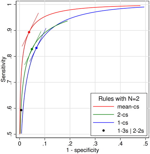
Figure 1. Receiver operating characteristic (ROC) curves for three families of quality control rules with N = 2 in the scenario of a 4 sigma analytical method: the mean-cs family (red), the 2-cs family (green), and the 1-cs family (blue). We varied c from 0.5 to 4.0 in steps of 0.01. Also shown is the single point in the ROC plane of the combined control rule 1-3s | 2-2s N2. The points on the three ROC curves represent control rules with the same likelihood ratio (LR) of 1.98, which is equal to the slopes of the curves at the points. The respective tangents are indicated. They are the mean-1.47s rule (red point), and the westgard rules 2-1.01s (green point) and 1-2.12s (blue point). Only the upper left quadrant is shown. The values of sensitivity and 1-specificity of the 4 points are: Red point, 0.894 and 0.0379. Green point, 0.825 and 0.0489. Blue point 0.832 and 0.0661. Black point, 0.593 and 0.00628.

The probability of alarm (sensitivity and 1 - specificity) was calculated as follows:

1-cs N2 family

$$\text{sensitivity}=\text{1}-{\left[\varphi \left(\text{c}-\text{2}.35\right)-\varphi \left(-\text{c}-\text{2}.35\right)\right]}^2$$

where ϕ(•) is the cumulative standard normal distribution where the mean is 0 and the standard deviation is 1.

Explanation: The expression ϕ(c) is the probability of getting 1 result between -∞ and c when the mean = 0. For instance, ϕ(1.96) = 0.975. When the mean is not zero, one has to subtract the mean in units of s in order to use the standard normal distribution. The expression ϕ(c − 2.35) is the probability of getting 1 result between -∞ and c when the mean = 2.35, while ϕ(-c − 2.35) is the probability of getting 1 result between -∞ and -c, so [ϕ(c − 2.35) - ϕ(-c − 2.35)] is the probability of getting 1 result in the interval -c to c. Then [ϕ(c − 2.35) - ϕ(-c − 2.35)]² is the probability of getting 2 results in the interval -c to c (i.e. the probability of no alarm), and 1 - [ϕ(c − 2.35) - ϕ(-c − 2.35)]² is the probability of getting no results in the interval, i.e. the probability of alarm. $$1\hspace{0.17em}-\text{\hspace{0.17em}specificity\hspace{0.17em}}=\text{\hspace{0.17em}1\hspace{0.17em}}-\hspace{0.17em}{\left[\varphi \left(c\right)\hspace{0.17em}-\hspace{0.17em}\varphi \left(-c\right)\right]}^2$$

Explanation: This is the same expression as for sensitivity, except that the mean is zero.

2-cs N2 family

$$\text{sensitivity}={\left[1-\varphi \left(\text{c}-\text{2}.35\right)\right]}^2+{\left[\varphi \left(-\text{c}-\text{2}.35\right)\right]}^2$$

Explanation: From what is written above, the expression [1 - ϕ(c − 2.35)] is the probability of getting 1 result above c, and [1 - ϕ(c − 2.35)]² is the probability of getting 2 results above c. The expression [ϕ(-c − 2.35)]² is the probability of getting 2 results below -c, and the sum of these expressions is the probability of getting 2 results above c or 2 results below -c, which is the probability of alarm. $$1\hspace{0.17em}-\text{\hspace{0.17em}specificity\hspace{0.17em}}=\hspace{0.17em}{\left[1\hspace{0.17em}-\hspace{0.17em}\varphi \left(c\right)\right]}^2+\hspace{0.17em}{\left[\varphi \left(-c\right)\right]}^2$$

Explanation: This is the same expression as for sensitivity, except that the mean is zero.

Mean-cs N2 family

$$\text{sensitivity}=\text{1}-\varphi \left[\left(\text{c}-\text{2}.35\right)\times {\text{2}}^{0.5}\right]+\varphi \left[\left(-\text{c}-\text{2}.35\right)\times {\text{2}}^{0.5}\right]$$

Explanation: This is the same expression as for the 1-cs N1 family (not shown above, but equal to the 1-cs N2 without quadration of the parenthesis), except that the standard deviation is reduced by the factor 2^0.5, because now we are using the standard deviation of the mean of 2 measurements. Consequently, the distance from c to 2.35, which is measured in standard deviations, becomes correspondingly larger. For example, if c = 1, the sensitivity is $$\begin{array}{c}\begin{array}{l}1\hspace{0.17em}-\hspace{0.17em}\varphi \left[\left(1\hspace{0.17em}-\text{\hspace{0.17em}2}.35\right)\hspace{0.17em}\times \hspace{0.17em}{2}^{0.5}\right]\hspace{0.17em}+\hspace{0.17em}\varphi \left[\left(-1\hspace{0.17em}-\text{\hspace{0.17em}2}.35\right)\hspace{0.17em}\times \hspace{0.17em}{2}^{0.5}\right]\hspace{0.17em}\\ =\text{\hspace{0.17em}1\hspace{0.17em}}-\hspace{0.17em}\varphi \left[-1.9091883\right]\hspace{0.17em}+\hspace{0.17em}\varphi \left[-4.7376154\right]\hspace{0.17em}=\end{array}\\ 1\hspace{0.17em}-\hspace{0.17em}0.0281189\hspace{0.17em}+\hspace{0.17em}0.000001081\hspace{0.17em}\approx \hspace{0.17em}\mathrm{0.97.}\end{array}$$ $$1\hspace{0.17em}-\text{\hspace{0.17em}specificity\hspace{0.17em}}=\text{\hspace{0.17em}1\hspace{0.17em}}-\hspace{0.17em}\varphi \left[\left(c\right)\hspace{0.17em}\times \hspace{0.17em}{2}^{0.5}\right]\hspace{0.17em}+\hspace{0.17em}\varphi \left[\left(-c\right)\hspace{0.17em}\times \hspace{0.17em}{2}^{0.5}\right]$$

Explanation: This is the same expression as for sensitivity, except that the mean is zero.

In addition, we also estimated sensitivity and 1 - specificity of the combined control rule 1-3s | 2-2s N2 by simulating 10 million runs at a systematic error of 2.35 s and at the normal state. ROC curves were plotted for each family of control rules. For the sake of comparison, we also made a Supplementary Figure of the ROC curve of 1-cs N1 and 1-cs N2 rules in the same scenario of a 4 sigma analytical method.

In analogy with diagnostic tests, the optimal control rule in each family corresponds to the optimal operating point on the ROC curve. For a diagnostic test, this point depends on the pretest probability of disease (pre), the benefit (B) of treating true positives and the cost (C) of treating false positives. The pretest probability in this setting is the probability of getting a systematic error as large as (or greater than) the critical systematic error. B is the benefit of diagnosing a systematic error as large as the critical systematic error, and C is the cost of falsely diagnosing it when it does not occur (false alarm). B and C must be seen in health-related units, as for instance quality-adjusted days. Then B is associated with avoiding analytical results that can harm the patients, and C is associated with unnecessarily delaying analytical results because the run has to be repeated.

The treatment threshold is the probability of disease above which some clinical action is preferred [12]. It is given by the expression 1/(1 + B/C) [12]. Posttest probability of disease is pre × LR/(pre × LR + 1 - pre), where LR is the likelihood ratio of the test result. LR is defined as the probability of getting a certain test result in a patient with disease divided by the probability of getting the same test result in a patient without disease. The optimal LR (LR_opt) that brings posttest probability to the level of the treatment threshold is given by the equation: $$\begin{array}{l}(\text{pre\hspace{0.17em}}\times \hspace{0.17em}{\text{LR}}_{\text{opt}}/\left(\text{pre\hspace{0.17em}}\times \hspace{0.17em}{\text{LR}}_{\text{opt}}+\text{\hspace{0.17em}1\hspace{0.17em}}-\text{\hspace{0.17em}pre}\right)\hspace{0.17em}=\text{\hspace{0.17em}1}/\left(1\hspace{0.17em}+\text{\hspace{0.17em}B}/C\right),\text{\hspace{0.17em}or\hspace{0.17em}}{\text{LR}}_{\text{opt}}\\ =\hspace{0.17em}\left[\left(1\hspace{0.17em}-\text{\hspace{0.17em}pre}\right)/\text{pre}\right]/\left[B/C\right].\end{array}$$

The cut-off value corresponding to LR_opt is the optimal cut-off value for diagnostic tests in a certain clinical setting. As the slope of the tangent of the ROC curve at a given point equals LR [13], the optimal operating point on the ROC curve is the point where the slope of the tangent of the ROC curve is equal to LR_opt. In analogy, the control rule that corresponds to the point on the ROC curve where the slope is equal to LR_opt, is the optimal rule in its family.

In order to compare E(N_UF) curves of the optimal rule from each of three families, we had to define an LR_opt. We defined pretest probability equal to 0.01 and B/C-ratio equal to 50, so that LR_opt was [(1 − 0.01)/0.01]/50 = 1.98. Those are just made-up numbers, chosen to show the principles. The optimal points on the three ROC curves were the points where the tangents had a slope equal to 1.98 (Figure 1).

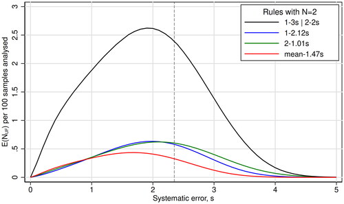
The three optimal control rules so defined were compared according to their E(N_UF) curves [10] along with the E(N_UF) curve of the combined control rule 1-3s | 2-2s N2 (Figure 2). E(N_UF) was calculated as in equation 2 in the paper of Yago & Alcover [14].

Figure 2. The curves show the expected increase in the number of unacceptable patient results reported during the presence of an out-of-control error condition, E(N_UF), per 100 patient samples analyzed, as a function of systematic error given in multiples of the stable analytical imprecision (s). Each curve represents one quality control rule. The maximal allowable total error is 4 s, so the critical systematic error is 2.35 s (stippled line).

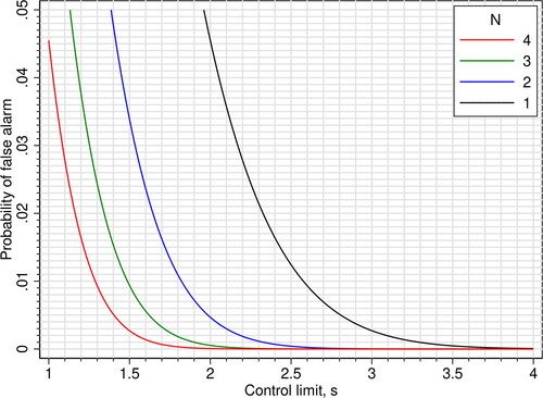
As a practical help in choosing mean rules, we constructed two figures: One figure that shows the control limit that gives a probability of 0.90 (90%) of detecting a critical systematic error (P_ed) for certain values of N and critical systematic error [8] (Figure 3), and one figure that shows the probability of false alarm (P_fr, false rejection) given the control limit and N (Figure 4). In the last figure, we used the expression 1 - specificity = 1 - ϕ[(c) × N^0.5] + ϕ[(-c) × N^0.5] to calculate the probability lines.

Figure 3. Mean rules: The y-axis shows the control limits giving a probability of alarm (probability of error detection; sensitivity) of 0.90 (90%) for errors equal to the critical systematic error. The control limits are plotted as functions of the critical systematic error and N. When N = 1, the mean rules are equal to Westgard 1-cs N1 rules. The corresponding probabilities of false alarm (false rejection; 1 - specificity) are shown in Figure 4.

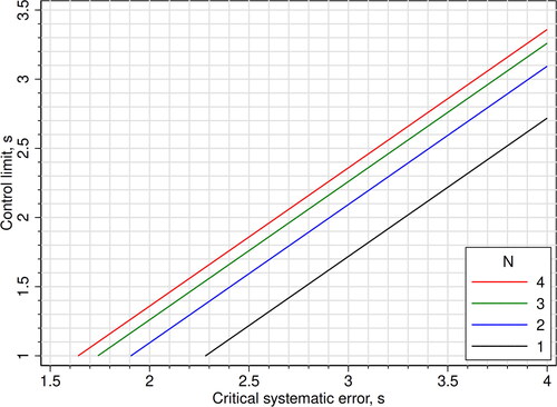
Figure 4. Mean rules: Probability of false alarm (false rejection; 1 - specificity), plotted as functions of the control limit and N. When N = 1, the mean rules are equal to Westgard 1-cs N1 rules.

Stata, version 16 (College Station, Texas 77845 USA) [15] was used for calculations and graphical work, except for fitting and derivation of the ROC curves where we used the software CurveExpert Professional, version 2.6.5 [16]. The software Statistics101, version 5.7 [17], was used for simulation.

Results

ROC curves for the three families of quality control rules are shown in Figure 1. Also shown is the single point of the combined control rule 1-3s | 2-2s N2. The uppermost ROC curve, representing the diagnostic most accurate family of rules, was that of the mean-cs N2 family. The point on this ROC curve with an LR of 1.98, which was defined as the optimal operating point, had a sensitivity of 0.894 and 1 - specificity of 0.0379. Its c-value was 1.47, so the point represented the quality control rule mean-1.47s N2. The second best ROC curve was that of the 2-cs N2 family, where the optimal point with an LR of 1.98 corresponded to the control rule 2-1.01s N2, with sensitivity of 0.825 and 1 - specificity of 0.0489. The third best ROC curve belonged to the 1-cs N2 family, where the optimal point with an LR of 1.98 corresponded to the control rule 1-2.12s N2, with sensitivity of 0.832 and 1 - specificity of 0.0661. The single point of the combined control rule 1-3s | 2-2s N2 had a sensitivity of 0.593 and 1- specificity of 0.00628. It was located slightly below the ROC curve of the 2-cs N2 family. The ROC curves of the 1-cs N1 and 1-cs N2 families are shown in the Supplementary Figure.

The E(N_UF) curves, i.e. the curves showing the expected increase in the number of unacceptable patient results reported during an out of control error condition, are shown in Figure 2. The combined control rule 1-3s | 2-2s N2 had the uppermost curve and, accordingly, the largest Max E(N_UF). The three other rules had clearly lower Max E(N_UF). The lowest of all curves belonged to the mean-1.47s N2 rule.

Figure 3 shows the control limit of various mean rules with a probability of 0.90 (90%) of detecting an error equal to the critical systematic error. The corresponding probabilities of false alarm are shown in Figure 4.

Discussion

This work shows that a given quality control rule for a given scenario with a defined critical systematic error can be represented by one point on a ROC curve (Figure 1 and Supplementary Figure). The whole curve describes the diagnostic accuracy of a family of rules that appear when only the control limit is varied. ROC curve analysis of the performance of quality control rules has been done previously. Pearson & Cawte studied the accuracy of Shewhart and cusum rules in monitoring quality control measurements of dual-energy X-ray absorptiometry (DXA) equipment [18]. However, they did not clearly define families of rules, and they did not elaborate on how to find the best rule in each family.

The most accurate family of rules is the family whose ROC curve lies above the others [9]. For instance, as shown in Figure 1, a mean rule should be chosen in preference to the 1-3s | 2-2s rule, because the ROC curve of that family is above the point of 1-3s | 2-2s rule. Even if the 1-3s | 2-2s rule has an acceptable risk of false alarm, there is a mean rule with the same probability of false alarm and a higher sensitivity, i.e. a better diagnostic accuracy. An obvious finding in this work is that the family of mean rules is more accurate than two families of Westgard rules in detecting systematic errors when N = 2. This has been shown before for a few rules [5–8], but not for an entire family of rules. Both Linnet [6] and Parvin [7] state that ‘it can be proved’ that a test (or rule) based on the mean is ‘the most powerful’ to detect a shift in the mean. Then our findings in the ROC curve analysis should come as no surprise and are expected to be similar for any N > 1.

Finding the best rule in each family, i.e. finding the optimal operating point on its ROC curve, ideally should be based on pretest probability, benefit and cost. The pretest probability, i.e. the probability of getting a systematic error as large as (or greater than) the critical systematic error, is quite low for a stable analytical method, perhaps 0.01 or lower for each run. The benefit (B) of diagnosing a systematic error as large as the critical systematic error is hard to estimate, and likewise the cost (C) of falsely diagnosing it when it does not occur (false alarm). It may be easier to consider the B/C-ratio. Most likely, the patients themselves would assign a greater value to B than to C, so from their point of view the B/C-ratio should be greater than 1. In the example in Figure 1, a B/C-ratio of 50 in combination with a pre of 0.01 lead to an LR_opt of 1.98 and a corresponding control rule with P_ed of 0.89 and P_fr of 0.038. From the formula of LR_opt (Methods) it is evident that a lower B/C-ratio would lead to a higher LR_opt and an optimal operating point at a steeper part of the ROC curve, because the LR equals the slope of the tangent of the ROC curve. Inevitably, this would correspond to a rule with a lower P_ed (sensitivity) and a lower P_fr (1 - specificity). On the other hand, a higher B/C-ratio would lead to a lower LR_opt, and an optimal operating point at a less steep part of the ROC curve corresponding to a rule with a higher P_ed and a higher P_fr. Note that these considerations apply to all families of rules, and that LR_opt is the same for all families. However, the same LR_opt leads to different P_ed and P_fr in different families (Figure 1). If LR_opt is located at a steeper or flatter part of the ROC curves, where the curves are closer to each other, the difference between the QC rules becomes less prominent than shown in Figure 1. Also note that the ROC curves may cross, as the curves of the 1-cs N2 and 2-cs N2 families in Figure 1, making the area under the curves less relevant than their actual positions.

Traditionally, laboratories have preferred control rules with a P_fr less than 0.01, i.e. far to the left on the ROC curve. The formula of LR_opt (Methods) shows that such rules are optimal only if pre is very low and/or the B/C-ratio is low.

There is at least one other consideration to be made when deciding on a statistical quality control procedure: The run size. For that purpose, it may be appropriate to calculate the Max E(N_UF). As shown in Figure 2, this patient risk parameter reaches its highest value at systematic errors lower than the critical systematic error. In the ROC curve analysis, that aspect is missing because ROC curve analysis uses only two points on the power function curves. However, also the use of Max E(N_UF) suffers from the lack of knowledge: We do not know the probability of getting a systematic error that corresponds to the Max E(N_UF), and we certainly do not know the amount of damage such relatively small errors might do to the patients.

In accordance with Yago & Alcover [14] we observed that the Max E(N_UF) is correlated with the probability to detect the critical systematic error. In their opinion, the use of control rules with a probability of 0.90 (90%) to detect critical systematic errors ‘reduce the probability of harming the patient to a level that could be considered acceptable for many tests conducted in a laboratory’ [14]. In Figure 2, the three rules with the same LR could be compared on equal grounds, because those rules are chosen from the same weighing of decision premises. So from this risk perspective also, a mean rule was the best. As the Max E(N_UF) is below 0.5 per 100 patients’ samples (Figure 2), the run size could increase to more than 200 for Max E(N_UF) to reach 1 for the mean-1.47s rule, a criterion used by Westgard & Westgard [19]. A lower criterion than 1, i.e. a smaller run size, would be more expensive. Anyway, a run size of 200 in a 4 sigma scenario is rather good, as it compares with a multirule with N = 4 [20].

Why then are mean rules hardly mentioned in textbooks [21] and seldom used in clinical chemistry laboratories? Linnet discussed this paradox in 1991 [6]. He thought that Westgard rules may be more easily applied, but also mentioned that computation of the mean could be no problem in the computerized laboratory. Now, more than 30 years later, mean rules should be even more easy to apply. It should also be very easy to have a computer calculate the control limit (i.e. the c-value) for an appropriate mean rule, because a mean rule basically is a 1-cs’ N1 Westgard rule where s’ = s/N^0.5 (Methods). A spreadsheet could do the job, or, in the case of finding the control limit of mean rules with a sensitivity of 0.90 (90%), Figure 3. Remarkably, with mean rules one gets a lower probability of false alarm by increasing N (Figure 4). The reason for the underuse of mean rules may be that vendors of instruments and middleware have not been asked to make the necessary software development because the laboratories feel (rightly or not) no need to improve on their quality control routines.

In this scenario we used a 4 sigma analytical method to illustrate the principles, which are, of course, not limited to just this scenario. A 4 sigma analytical method was chosen because it is neither bad nor excellent, and may be representative for methods where rules based on just 1 control measurement is insufficient (Supplementary Figure). If rules with N = 1 are sufficient, there is no point in searching for rules with N > 1. However, the principles of finding the optimal rule by identifying the LR_opt is equally valid when N = 1. We did not elaborate on the practical aspects of quality control, for instance where in the run to place the control material. We also concentrated on systematic errors, and did not discuss worsened imprecision. Linnet [6] recommended variance rules to detect worsened imprecision.

Conclusions: For a given scenario with a defined critical systematic error, quality control rules are represented by points on the ROC curve of their family. For N > 1, the most accurate families in detecting systematic errors are those of mean rules. The best rule in a family can be identified as the one represented by the optimal operating point on the ROC curve. If rules with N = 1 are insufficient, choose a mean rule. If the optimal operating point on the ROC curve cannot be determined, choose a mean rule with a sensitivity of 0.90 (90%) which secures a sufficiently low Max E(N_UF), and choose a probability of false alarm as low as practically and economically achievable.

Disclosure statement

No potential conflict of interest was reported by the author(s).

References

- Kinns H, Pitkin S, Housley D, et al. Internal quality control: best practice. J Clin Pathol. 2013;66(12):1027–1032. doi:10.1136/jclinpath-2013-201661.
- Laubender RP, Geistanger A. Selection of within-run quality control rules for laboratory biomarkers. Stat Med. 2021;40(16):3645–3666. doi:10.1002/sim.8987.
- Westgard JO. Internal quality control: planning and implementation strategies. Ann Clin Biochem. 2003;40(Pt 6):593–611. doi:10.1258/000456303770367199.
- Gowans EM, Hyltoft Petersen P, Blaabjerg O, et al. Analytical goals for the acceptance of common reference intervals for laboratories throughout a geographical area. Scand J Clin Lab Invest. 1988;48(8):757–764.
- Westgard JO, Groth T. Power functions for statistical control rules. Clin Chem. 1979;25(6):863–869. doi:10.1093/clinchem/25.6.863.
- Linnet K. Mean and variance rules are more powerful or selective than quality control rules based on individual values. Eur J Clin Chem Clin Biochem. 1991;29(7):417–424. doi:10.1515/cclm.1991.29.7.417.
- Parvin CA. New insight into the comparative power of quality-control rules that use control observations within a single analytical run. Clin Chem. 1993;39(3):440–447. doi:10.1093/clinchem/39.3.440.
- Asberg A, Bolann B, Mikkelsen G. Using the confidence interval of the mean to detect systematic errors in one analytical run. Scand J Clin Lab Invest. 2010;70(6):410–414. doi:10.3109/00365513.2010.501114.
- Metz CE. Basic principles of ROC analysis. Semin Nucl Med. 1978;8(4):283–298. doi:10.1016/s0001-2998(78)80014-2.
- Parvin CA. Assessing the impact of the frequency of quality control testing on the quality of reported patient results. Clin Chem. 2008;54(12):2049–2054. doi:10.1373/clinchem.2008.113639.
- Westgard S, Bayat H, Westgard JO. Analytical sigma metrics: a review of six sigma implementation tools for medical laboratories. Biochem Med (Zagreb). 2018;28(2):020502. doi:10.11613/BM.2018.020502.
- Pauker SG, Kassirer JP. Therapeutic decision making: a cost-benefit analysis. N Engl J Med. 1975;293(5):229–234. doi:10.1056/NEJM197507312930505.
- Choi BC. Slopes of a receiver operating characteristic curve and likelihood ratios for a diagnostic test. Am J Epidemiol. 1998;148(11):1127–1132. doi:10.1093/oxfordjournals.aje.a009592.
- Yago M, Alcover S. Selecting statistical procedures for quality control planning based on risk management. Clin Chem. 2016;62(7):959–965. doi:10.1373/clinchem.2015.254094.
- http://www.stata.com
- http://www.curveexpert.net
- http://www.statistics101.net
- Pearson D, Cawte SA. Long-term quality control of DXA: a comparison of shewhart rules and cusum charts. Osteoporos Int. 1997;7(4):338–343. doi:10.1007/BF01623774.
- Westgard JO, Westgard SA. Establishing Evidence-Based statistical quality control practices. Am J Clin Pathol. 2019;151(4):364–370. doi:10.1093/ajcp/aqy158.
- Westgard SA, Bayat H, Westgard JO. Selecting a risk-based SQC procedure for a HbA1c total QC plan. J Diabetes Sci Technol. 2018;12(4):780–785. doi:10.1177/1932296817729488.
- Miller W, Sandberg S. Quality control of the analytical examination process. In: Rifai N, Horvath AR, Wittwer CT, editors. Tietz textbook of clinical chemistry and molecular diagnostics. 6th ed. St. Louis: Elsevier; 2018. p. 121–156.