Catchment topography and the distribution of electron donors for denitrification control the nitrate concentration in headwater streams of the Lake Hachiro watershed

ABSTRACT

We examined the linkages between topography and electron donors for denitrification on in-stream NO₃⁻ concentration in headwater catchments in the Lake Hachiro watershed having marine sedimentary rock, Japan. In 35 headwater catchments (0.07–16.9 km²), we sampled stream water every season in 2 years. The water samples were analyzed for NO₃^–, dissolved nitrous oxide (dN₂O), and SO₄^{2 –} concentrations. Stream sediment was sampled once for the measurement of denitrification potential (DP). Water-extractable soil organic carbon (WESOC) and easily oxidizable sulfide (EOS) in the sediment, which can be considered the principal potential electron donors for denitrification, were measured. The topographical features of each catchment were calculated using a digital elevation model with 10-m grid cells. Stream NO₃ ^– concentrations displayed large spatial variation among catchments, ranging from 0.06 to 0.52 mg N L^–1, and were negatively correlated with topographic wetness index (TWI) (P < 0.01) and were positively correlated with catchment slope (P < 0.01), indicating that NO₃ ^– concentrations decreased in wetter and gentle slope catchments. Sediment DP and the WESOC content in sediments were positively correlated with TWI, significantly. These results suggested denitrification was likely to occur in higher TWI catchments. Generalized linear model showed that TWI, slope aspect, and sediment DP significantly affected in-stream NO₃ ^– concentration and WESOC was a significant explanatory variable for sediment DP. EOS content in riverbed sediments was not selected as a significant explanatory variable for either in-stream NO₃⁻ concentrations or sediment DP. But higher soil DP with higher EOS was detected in the stream bank subsoil at the catchment where the higher EOS content in the riverbed sediment was observed, which suggested EOS in riverbed sediments can contain site-specific information about denitrification hotspot driven by sulfides. We conclude that catchment topography and the distribution of electron donors in riverbed sediment can be important factors to explain the spatial variation in in-stream NO₃ ^– concentration and sediment DP.

KEYWORDS:

• topography
• coastal area
• riparian
• sulfur denitrification
• biogeochemical hot spot

1. Introduction

Human activities dramatically increased the amount of reactive nitrogen (N) in global ecosystems and have increased food production; but the greater input of reactive N beyond appropriate uses can lead to eutrophication of surface water, causing degradation of aquatic ecosystems and problem such as toxic algal blooms, loss of dissolved oxygen, depletion of fish populations, and biodiversity loss (Galloway and Cowling 2002; Vitousek et al. 1997; Carpenter et al. 1998). Previous mass balance studies conducted to evaluate the fate of reactive N in watersheds frequently fails to account for a large proportion of the N, and part of this ‘missing N’ is considered to represent the fraction that undergoes transfer to the atmosphere by denitrification (Boyer et al. 2006; Hayakawa et al. 2009; Howarth et al. 1996; Kimura et al. 2012). Denitrification is the anaerobic reduction of N oxides to nitrogenous gases, generally by particular groups of ubiquitous heterotrophic bacteria that have the ability to use NO₃ ^– as an electron acceptor and organic carbon (C) as an electron donor during anaerobic respiration. The main factors controlling denitrification rates, therefore, are the supply of organic C, NO₃^–, and oxygen (Tiedje 1994). Because denitrification removes reactive N finally as N₂ gas from the ecosystem, it is a highly valued ecosystem service in N-enriched watersheds (Craig et al. 2008), but an extremely challenging process to measure and model (Groffman et al. 2009).

Landscape topography can control biogeochemical N cycles such as denitrification. At sites with a relatively flat topography, the low hydraulic gradient increases water residence time in the riparian zone and enhances the development of anaerobic conditions necessary for denitrification (Vidon and Hill 2004). Microtopography within riparian zones has a significant influence on soil oxygen dynamics and therefore redox-sensitive biogeochemical processes such as denitrification (Duncan, Groffman, and Band 2013). Topography represented by a digital elevation model (DEM) has been used to predict the spatial distribution of the microbial biomass and the amount of denitrifying enzymes in the soil at the plot scale (Florinsky, McMahon, and Burton 2004). Despite much effort and many studies at plots and microtopographic scales showing the effects of elevation and topography on soil denitrification potential (DP) within riparian forests (Harms and Grimm 2008; Ullah and Faulkner 2006), limited research has been conducted at broader landscape scales. A significant negative correlation was found between topographic index (wetness index) calculated from a DEM and in-stream NO₃ ^– concentration in a catchment (Ogawa et al. 2006); but the causal relationship was unclear. Duncan, Groffman, and Band (2013), using DEM analysis and field-monitoring of soil moisture and oxygen concentration in the soil air, found that the importance of denitrification in the N budget of forested watersheds appeared to depend fundamentally on the presence of landscape elements such as riparian hollows that function as hot spots of denitrification activity. Hayakawa et al. (2012) showed in a landscape-scale study that low-elevation riparian forest soils had a higher DP due to their higher contents of moisture, clay, and water-extractable soil organic carbon (WESOC), and that these factors appeared to reduce riverine NO₃ ^– concentration. However, the observations of relations between catchment topography and in-stream NO₃⁻ or its related denitrification variables such as sediment DP in headwater catchments is still lacking.

Generally, organic C is known as the primary electron donor for denitrification in ecosystems, but electron donors other than organic C can also drive denitrification. Some bacteria can use inorganic sources, such as reduced sulfur compounds and Fe²⁺, as the electron donor to grow chemoautotrophically (Korom 1992; Straub et al. 1996). The oxidation of such inorganic species coupled with N oxide reduction is termed autotrophic denitrification. A number of previous studies have revealed NO₃ ^– removal coupled with sulfide oxidation in groundwater systems (Craig, Bahr, and Roden 2010; Jørgensen et al. 2009; Postma et al. 1991; Schwientek et al. 2008), in riverbed sediments (Hayakawa et al. 2013; Yang et al. 2012), and in sediment incubated with added sulfur (Brunet and Garcia-Gil 1996; Garcia-Gil and Golterman 1993; Jørgensen et al. 2009; Torrentó et al. 2010, 2011). NO₃⁻ reduction coupled with sulfide oxidation could be widespread and biogeochemically important in freshwater sediments (Burgin and Hamilton 2008). However, the relative importance of the electron donors in the removal process remains uncertain at watershed scales.

The extent of NO₃ ^– reduction in aquifers at the watershed scale depends on both the hydrogeological conditions and the availability of electron donors (Postma et al. 1991). However, spatial hot spots of denitrification are relatively undetectable due to our inability to obtain sufficiently high spatial resolution of the distribution of denitrification drivers (electron donors) because of their heterogeneous vertical and horizontal distribution (Groffman et al. 2009). The composition of riverbed sediment can integrate the surface soil and geology variation of a catchment and has been used to identify site that shows distinctive water quality (Horowitz and Elrick 2017) and to construct geochemical maps (Imai et al. 2004). We hypothesize that the amount of electron donors for denitrification present in riverbed sediments might also represent the relative amount in the catchment. That is, the strength of denitrification in a catchment might be explained by the amount of electron donors in riverbed sediments and the catchment’s topographic features.

One of the special characteristics of the Lake Hachiro watershed (LHW) that is our study site is its geology. The region was submerged beneath the sea during the Neogene period (Shiraishi and Matoba 1992), so sulfide minerals are expected to be distributed throughout the watershed including forest area in upper mountain because sulfides are generally produced in marine systems (Richkard and Luther 2007). High sulfide content could be reasonably expected to influence the N cycle through sulfur denitrification. However, NO₃ ^– concentrations in the headwater streams of the watershed and the mechanisms of NO₃ ^– removal have not previously been studied. The hypothesis of this study was that the interaction between topographic factors and availability of electron donors for denitrification controls in-stream NO₃ ^– concentrations. To test this hypothesis, we evaluated the effects of catchment topography and amounts of organic C and reduced sulfur in riverbed sediments on in-stream NO₃ ^– concentration and riverbed sediment denitrification potential in 35 headwater catchments of the LHW, Akita prefecture, Japan.

2. Materials and methods

2.1. Site description

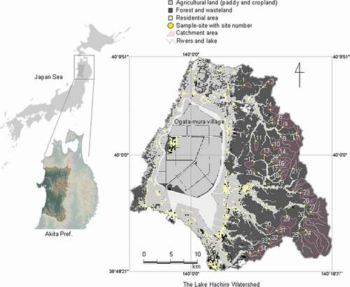
The LHW is located in western Akita prefecture facing the Japan Sea (Figure 1). The entire watershed area is 894 km². Lake Hachiro previously had a surface area of 220 km² and was the second largest lake (Hachirogata) in Japan before the implementation of the Hachirogata National Land Reclamation Project, which was designed to improve self-sufficiency in food production in Japan (Ogata-mura village office; Sasaki 2010). As part of the Project, Japan’s largest polder, Ogata-mura village, was constructed, reclaiming about four-fifth of the area of the lake and transforming the lake water from brackish to fresh. Because of the lake water eutrophied after the reclamation, Lake Hachiro was designated in 2007 under the Law Concerning Special Measures for Conservation of Lake Water Quality in Japan (Kondo 2010; Sasaki 2010). Therefore, the need to improve its water quality is considered urgent and it is also important to understand the mechanism for the formation of natural water at the forested area in the LHW.

Figure 1. Location of the Lake Hachiro watershed (LHW), Akita, Japan, and the land-use distribution and location of studied headwater catchments and sampling sites within the watershed

Average weather recordings for the region from the Gojome recording station for the period 1981–2010 (Japan Meteorological Agency 2013) reveal that precipitation averages 1553 mm year^–1 and the annual mean temperature is 10.8°C. The lowest mean monthly temperature occurs in January (–0.9°C) and the highest mean monthly temperature in August (24°C). The average maximum snow depth during winter (December–February) is 48 cm. The elevation in the LHW ranges from – 6.3 m inside the polder to 1037 m above sea level and is generally higher in the southern part than in the northern part of the forested area of the watershed (Figure 1). Japanese cedar (Cryptomeria japonica D. Don) plantations dominate the forested area, especially in the middle and northern parts of the watershed. Deciduous broadleaf forest also occurs in the southern forested portion of the watershed (Biodiversity Center of Japan, Nature Conservation Bureau, Ministry of the Environment).

The geological strata of the watershed belong to the Green Tuff zone, consisting of volcanic rocks and sedimentary rocks of the later Miocene (Shiraishi 1990). In the early Middle Miocene, the Akita region was drowned as a result of subsidence of previous land areas. The Oga Peninsula, where Lake Hachiro is located, was under deep water in the Early to Middle Pleistocene and later became a shallow marine shelf in the late to Middle Pleistocene (Shiraishi and Matoba 1992). As a result, the sedimentary rocks in the LHW are mainly marine deposits and comprise thick mudstone layers (Shiraishi 1990).

We established sample sites for the determination of water quality at positions that then defined the outlet of 35 headwater catchments of the five main rivers entering Lake Hachiro (Figure 1). Each catchment was independent (i.e., none are nested within or overlap others) and all were forested. The geography and topography of each catchment were characterized using a DEM of 10 m × 10 m resolution (Geospatial Information Authority of Japan) using the GIS software TNTmips Pro 2015 (Microimages Inc., Lincoln, NE, USA). The catchment geographical and topographical characteristics are summarized in Table S1. Topographic wetness index (TWI, Beven and Kirkby 1979) is commonly used as an indicator of soil wetness within a catchment. We determined TWI from the DEM using computer algorithms developed by Quinn, Beven, and Lamb (1995) and Beven (1997). The higher values of TWI infer a lower hydraulic gradient and greater upslope contributing area, that is, wetter soil conditions (Beven and Kirkby 1979). We calculated TWI for each 10 m × 10 m cell of the catchment and expressed topography as the median TWI of all cells in the catchment and the point TWI (pTWI) of the cell that is water sampled point (Table S1). Median elevation, median slope, median slope aspect (NS and EW) in each catchment were also calculated (see Table S1). Slope aspect was transformed from the circular data (0°-360°) to a value between 0 and 1 by the cosine transformation (McGrigal 2018). The transformation will return values of slope aspect_NS or slope aspect_EW approach 1 as the angles approach the north or the east and 0 as the angles approach the south or the west from either direction, respectively. We used the median value of all the cells in each catchment for the topographical characteristics because many of them did not follow the normal distribution.

2.2. Water, sediment, and soil sampling

Stream water samples were collected nine times – December 2009 and May, July, September, and December of 2010 and 2011 – from the 35 sample sites in the LHW. The sampling times were intended to represent seasonal conditions of winter, spring, summer, and autumn. To minimize any temporal variation at each sampling time, stream water samples were collected from all sites within a period of 3 days during base flow conditions as much as possible. The discharge (m³ s^–1) and specific discharge (m³ s^–1 km^–2) of each catchment was also measured at each sampling. The discharge was calculated by multiplying the cross-sectional area of the stream by the flow velocity. The cross-sectional area of the stream was calculated by multiplying the width of the stream by the depth. We divided the cross-section of the stream to 8–10 sections and measured the depth and the flow velocity (VP1000, KENEK, Co., Ltd., Tokyo) at each section. The cross-sectional area and the discharge of the stream were calculated by summing all the areas and the discharge of each section, respectively. Mean water velocity was calculated by dividing the discharge by the cross-sectional area of each stream.

Mean DIN (dissolved inorganic nitrogen; NO₃⁻ and NH₄⁺) atmospheric deposition measured at site No. 15 and 25 from 2010 to 2011 was 7.5 kg N ha⁻¹ yr⁻¹, which was higher than the threshold value of 5 kg N ha⁻¹ yr⁻¹ causing N leaching to stream in China (Fang et al. 2011) having a relatively similar Asian monsoon climate to Japan. The 2-year water-weighted mean N concentration in the atmospheric deposition were 0.32 mg N L⁻¹ for DIN, 0.18 mg N L⁻¹ for NO₃⁻, 0.14 mg N L⁻¹ for NH₄⁺. We assumed that the mean DIN bulk deposition measured at the two sites inputs evenly in all catchments.

Sediment samples from the riverbed of each sample site were obtained once in July 2011 at the same time as water sampling. We collected the samples from the 0–5 cm depth at over 10 random locations from the riverbed at the sample site within a range of about 20 m stream-length and sieved them to under 2.0 mm on site, and then combined the samples into a bulked sample for analysis. Due to forest road works preventing access to site No. 29 and deep water at site No. 34, sediment samples could not be collected from these two sample sites.

To evaluate a vertical distribution pattern of easily oxidizable-sulfur (EOS) at a stream bank, soil samples at site No. 15 where the riverbed EOS content was relatively high were collected by shovel at depths of 0–30, 30–60, 60–90, 90–120, 120–150, 150–180, and 180–210 cm in February 2014. The soil around high EOS content at the stream bank was sampled again in September 2015 for the evaluation of denitrification potential.

2.3. Chemical analysis of water, sediment, and soil samples

After sampling, the water, sediment, and soil samples were stored on ice until they could be transported to the laboratory, where they were then stored at 4°C until they were analyzed. The water samples were filtered through a 0.45-μm membrane filter (cellulose acetate, ADVANTEC, Japan). We measured the NO₃ ^– and SO₄2 –concentrations in the water using an ion chromatograph (DX-120, Dionex, Sunnyvale, CA, USA). The fresh sediment and soil samples were shaken with distilled water (soil:water, 1:5, w/v) for 60 min at 100 rpm at room temperature. The supernatant was filtered through a 0.45-μm membrane filter (cellulose acetate, ADVANTEC, Japan) and was sampled for the analysis after 5 mL discharged filtered solution. The extracts were used for the determination of dissolved organic C (DOC) concentration using a total organic C analyzer (TOC-5000, Shimadzu, Kyoto, Japan) and then WESOC content in the sediment and soil was determined. The DOC leached from the filter used in this study did not affect the measured values so largely (4.3 ± 4.3%, n = 33). EOS content in the sediment and soil samples was determined by the difference between H₂O₂-soluble sulfur (H₂O₂-S) and water-soluble sulfur (H₂O-S) contents (Murano, Yamanaka, and Mizota 2000).

2.4. Measurement of denitrification potential

The denitrification potential (DP) of sediment and soil samples was measured to quantify the variation among sites in the amount of electron donors available to denitrifying organisms. We defined DP as the denitrification rate that occurred under anaerobic conditions with abundant NO₃ ^– at 25°C and measured it using acetylene inhibition assay, which inhibits the final step in the conversion of N₂O gas into N₂ gas (Tiedje 1994). All DP assays were conducted within 3 days of sample collection. Samples of fresh, homogenized sediment (15 g) were placed into 150-mL glass bottles in triplicate. A 50-mL aliquot of solution containing nitrate (5 mg-N L^–1 as KNO₃) and chloramphenicol (6 mM, 97 mg bottle⁻¹) was added to the bottles, which were then closed with a butyl rubber septum and aluminum crimp. Two stainless needles (TERUMO, 23 G × 32 mm, and GL science, 19 G × 100 mm) were fastened to each septum and fitted with sterile three-way stopcocks. To achieve anoxic condition, O₂-free ultrapure N₂ gas was bubbled through the solution for 5 min, at the same time purging the headspace of air. After that, acetylene (C₂H₂) gas was added to the headspace to a final concentration of 10% v/v (10 kPa). We extracted the headspace gas with a gas-tight syringe at 6 h after adding the acetylene and calculated the denitrification rate from the linear portion of the curve for N₂O production as a function of time. Sediment DP was calculated from the following equations:

DP = ΔN_g/(M × Δt)Eq. (1)

N_g = [ρ × C × (V_g + αV_L)] × [273/(273 + T)]Eq. (2)

where DP is the sediment DP (µg N kg^–1 h^–1), ΔN_g is the change in weight of N₂O (N_g) in the incubation bottle (µg N₂O-N), M is the dry weight of sediment (kg), Δt is the incubation time (h), ρ is the density of N₂O under standard temperature and pressure (1.25 g N₂O-N L^–1), C is the concentration of N₂O (ppmv), V_g is the headspace of the incubation bottle (L), V_L is the liquid volume (L), α is the Bunsen coefficient (0.544 at 25°C; Tiedje 1994), and T is the temperature (°C) at which the gas samples were collected. N₂O was determined using a GC-14B gas chromatograph with an electron-capture detector (Shimadzu). Values of DP were reported on a dry-weight basis (µg N kg^–1 h^–1).

2.5. Measurement of dissolved N₂O

The concentration of dissolved N₂O (dN₂O) in stream water was measured once in July 2011, at the same time as sediment DP measurements, by using a headspace technique based on the principle of vapor–liquid equilibrium (Minamikawa et al. 2011; Sawamoto et al. 2003). We collected 25 mL of stream water using a 50-mL syringe in triplicate without degassing, and filled the rest of the syringe with 25-mL of O₂-free ultrapure N₂ gas from a Tedlar bag. After 3 min of vigorously shaking the syringes by hand to produce equilibrium between the vapor and liquid phases, the headspace gas was transferred from the syringe into a 15-mL evacuated glass vial. The concentrations of N₂O in the headspace gas were analyzed by using the gas chromatograph described above. The concentrations of dN₂O in the stream water were calculated based on Henry’s law considering measured water temperature (Sawamoto et al. 2003). The mean stream-water temperature at all the sample sites on that day was 6.1 ± 0.8°C. The dissolved N₂O concentration of the atmospheric N₂O equilibrium was 0.34 µg N L⁻¹ at 10°C.

2.6. Statistical analysis

We compiled available 22 variables data (see Fig. S1) on geographical and topographical features, environmental variables (stream water and sediment qualities), and stream properties from 33 sample sites except for two sites where sediment samples could not be sampled at No. 29 and No. 34, and analyzed them for the multivariate statistical analysis. As the shape of the histograms and the results of Shapiro-Wilk test of each variable data, some variables did not follow the normal distribution (see Fig. S1), the correlations between variables were evaluated by Spearman’s rank correlation coefficient.

To evaluate the factors influencing the spatial variation of in-stream NO₃⁻ concentration, generalized linear models (GLMs) were used. GLM was used to test the explicative power of the variables on spatial variation of in-stream NO₃⁻ concentration and sediment DP, respectively. Assuming that the error structure of the objective variable NO₃⁻ concentration and sediment DP follows gamma distribution, model selection was conducted with the minimum AIC (Akaike Information Standard) by the stepwise method (increase/decrease method) based on AIC. A log link function was used in each model. These statistical analyses were performed using R (R Development Core Team 2018, version 3.4.3).

3. Results

3.1. Spatio-temporal variations of in-stream NO₃ ^– concentration and its relations with topographic features in the LHW

Mean NO₃ ^– concentrations in the headwater streams displayed large spatial variation (Figure 2(a)), ranging from 0.06 to 0.52 mg N L^–1, and had an overall mean and median of 0.23 and 0.22 mg N L^–1, respectively (Table S2). NO₃⁻ was a main form of in-stream DIN (NO₃⁻ + NH₄⁺) and accounted for 90 ± 7.9% of DIN (Table S2). In most seasons, NO₃ ^– concentrations were significantly related to topographic factors (Table 1). Mean in-stream NO₃ ^– concentration was strongly correlated with the catchment median slope (r = 0.674, P < 0.01) and median TWI (r = – 0.554, P < 0.01), elevation (r = 0.427, P < 0.01). Mean in-stream NO₃ ^– concentration was not related to catchment size, latitude, longitude, slope aspect (NS and EW), pTWI, respectively. However, in some seasons, latitude, slope aspect (NS and EW) were correlated with in-stream NO₃ ^– concentration, significantly (Table 1).

Table 1. Spearman’s correlation coefficients at each sampling for the relationship between in-stream NO₃ ^– concentration and five geographic and topographic factors of 35 headwater catchments of the Lake Hachiro watershed

	n		Catchment size		Latitude		Longitude		Elevation (median)		Slope aspect_NS (median)		Slope aspect_EW (median)		Slope(median)		TWI(median)		TWI(point)
Dec-09	35		−0.039		−0.254		−0.125		0.171		0.254		−0.055		0.358	*	−0.340	*	−0.125
May-10	35		−0.091		−0.163		−0.079		0.189		0.417	*	−0.103		0.268		−0.302		−0.257
Jul-10	35		−0.233		−0.062		−0.041		0.095		0.051		−0.130		0.485	**	−0.597	**	−0.367	*
Sep-10	35		−0.015		0.140		0.128		0.181		0.203		−0.371	*	0.187		−0.143		−0.277
Dec-10	35		−0.039		−0.471	**	0.100		0.366	*	0.264		−0.408	*	0.619	**	−0.563	**	−0.282
May-11	34	†	−0.025		−0.487	**	0.237		0.490	**	0.281		−0.385	*	0.806	**	−0.703	**	−0.232
Jul-11	34	†	0.277		−0.365	*	0.303		0.582	**	0.446	**	−0.349	*	0.556	**	−0.203		−0.091
Sep-11	34	†	0.131		−0.255		0.353	*	0.591	**	0.529	**	−0.129		0.560	**	−0.149		−0.023
Dec-11	34	†	0.040		−0.380	*	0.321		0.450	**	0.319		−0.445	**	0.679	**	−0.561	**	−0.285
All	35		0.038		−0.288		0.212		0.427	**	0.328		−0.279		0.674	**	−0.554	**	−0.279
*, P < 0.05; **, P < 0.01
†Owing to road works, water samples could not be collected at sample site No. 29.

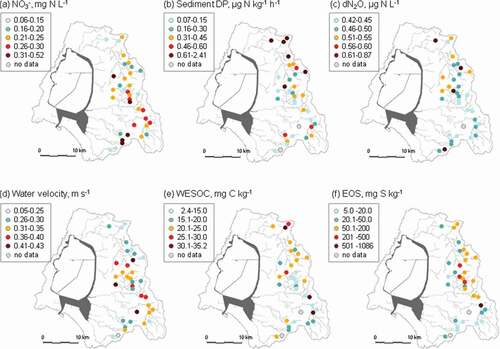
Figure 2. Spatial distribution of (a) mean NO₃ ^– concentration, (b) denitrification potential (DP) of riverbed sediment, (c) in-stream dissolved N₂O concentration (dN₂O), (d) mean water velocity, (e) water-extractable carbon (WESOC) content of riverbed sediment, and (f) easily oxidizable sulfur (EOS) content of riverbed sediment at the outlets of headwater catchments of the Lake Hachiro watershed

3.2. Spatial variation in sediment DP, water parameters, and electron donors for denitrification

The sediment and stream water parameters other than NO₃ ^– also displayed spatial variation (Figure 2). Sediment DP, dN₂O, and WESOC tended to be higher (Figure 2(b,c,e)) and water velocity tended to be lower (Figure 2(d)) in the northern part of the watershed. The dN₂O concentration in stream water ranged from 0.42 to 0.87 µg N L⁻¹ and were all higher than the dN₂O concentration of the atmospheric N₂O equilibrium (0.34 µg N L⁻¹ at 10°C). EOS content varied greatly among the catchments, ranging from 5.0 to 1086 mg S kg^–1, and displayed the highest values in the middle and northern part of the watershed (Figure 2(f)). The correlation between WESOC and EOS content in sediment was not significant (r = – 0.133, P = 0.46, Table S3).

3.3. Correlations between the variables

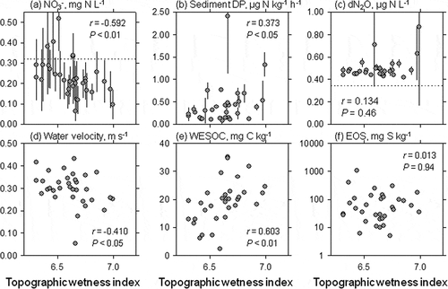
The catchment TWI was strongly related to several variables in the headwater streams of the watershed (Figure 3, Table S3; n = 33). A significant negative relationship was found between median TWI in catchment and in-stream NO₃ ^– concentration (r = −0.592, P < 0.01; Figure 3(a)). On the other hand, median TWI was positively correlated with sediment DP (r = 0.373, P < 0.05) and WESOC content (r = 0.603, P < 0.01), (Figure 3(b,e)). No significant relationship was found between median TWI and EOS (r = 0.013, P = 0.94, Figure 3(f)).

Figure 3. Relationships between median slope and (a) in-stream NO₃ ^– concentration (the dashed line indicates the water-weighted mean DIN concentration in the bulk deposition, 0.32 mg N L⁻¹), (b) denitrification potential (DP) of riverbed sediment, (c) in-stream dissolved N₂O concentration (dN₂O) (the dashed line indicates the ambient N₂O concentration, 0.34 µg N L⁻¹, 10°C), (d) mean water velocity, (e) water-extractable carbon (WESOC) content of riverbed sediment, and (f) easily oxidizable sulfur (EOS) content of riverbed sediment at the outlets of headwater catchments of the Lake Hachiro watershed (n = 33). Error bars represent standard deviation

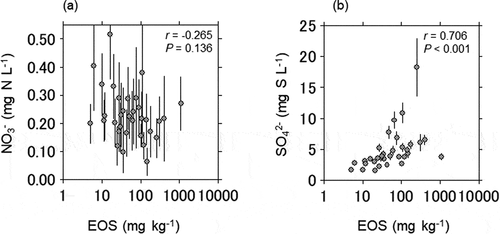
Sediment DP negatively correlated with in-stream NO₃⁻ concentration (r = −0.523, P < 0.01) and water velocity (r = −0.498, P < 0.01), and positively correlated with WESOC (r = 0.492, P < 0.01) and latitude (r = 0.538, P < 0.01) (Figure 4). NO₃ ^– concentration tended to decrease (r = – 0.265, P = 0.136) with EOS content (Figure 5(a)), and SO₄^{2 –} concentration increased significantly with EOS content (r = 0.706, P < 0.001; Figure 5(b)).

Figure 4. Relationships between (a) in-stream NO₃ ^– concentration, (b) mean water velocity, (c) water-extractable carbon (WESOC) content of riverbed sediment, (d) latitude, and denitrification potential (DP) of riverbed sediment at the outlets of headwater catchments of the Lake Hachiro watershed (n = 33). Error bars represent standard deviation

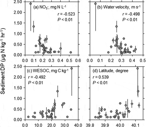
Figure 5. Relationships between easily oxidizable sulfur (EOS) content of riverbed sediment and (a) in-stream NO₃ ^– concentration, and (b) in-stream SO₄^{2 –} concentration at the outlets of headwater catchments of the Lake Hachiro watershed (n = 33). Error bars represent standard deviation

3.4. Generalized linear model analysis

Summary statistics of 22 variables and the results of the GLMs were shown in Tables 2 and 3, respectively. As a result of model selection based on AIC in the GLM analysis, the six explanatory variables (median TWI, median slope aspect_EW, median slope aspect_NS, pTWI, stream pH, and sediment DP) were identified as significant predictors of in-stream NO₃⁻ concentration (Table 3, model 1). For sediment DP, three explanatory variables such as water velocity, WESOC, and latitude were selected as significant predictors (Table 3, model 2). Excluding the latitude for the analysis, AIC value increased 1.2 and another two variables (dN₂O and discharge rate) were selected (Table 3, model 3).

Table 2. Summary statistics of 22 variables at the headwater catchments of the Lake Hachiro watershed (n = 33)

	median	max	min	25% quartile	75% quartile
Stream NO3^−, mg N L^−1	0.217	0.517	0.064	0.171	0.270
Sediment DP, µg N kg^−1 hr^−1	0.302	2.41	0.074	0.140	0.474
dN2O, µg L^−1	0.474	0.869	0.419	0.448	0.503
Catchment size, km^2	1.98	16.9	0.07	1.54	3.46
Latitude	39.98	40.12	39.84	39.90	40.03
Longitude	140.19	140.26	140.12	140.169	140.222
Elevation, m	162	477	66	135	220
Slope aspect_NS	0.491	0.638	0.305	0.448	0.561
Slope aspect_EW	0.379	0.835	0.206	0.329	0.465
Slope, deg	26	35	15	22	31
TWI	6.6	7.0	6.3	6.5	6.7
pTWI	18	20	14	16	18
Stream depth, m	0.12	0.30	0.036	0.095	0.18
Stream width, m	2.25	10.09	0.89	1.75	3.04
Water velocity, m s^−1	0.300	0.431	0.054	0.261	0.336
Discharge rate, m^3 s^−1 km^−2	0.048	0.182	0.016	0.038	0.053
Water temp., deg	11.9	13.4	10.0	11.4	12.5
pH	7.12	7.86	6.22	6.86	7.29
EC, mS m^−1	12.3	31.4	7.41	10.7	13.3
EOS, mg kg^−1	46.9	1086	4.97	24.7	108
WESOC, mg kg^−1	19.4	35.2	2.41	13.6	22.4
Stream SO4^2-, mg L^−1	3.86	18.3	1.61	3.03	5.36

Table 3. Results of a generalized linear model (GLM) for explaining the variance in-stream NO₃ ^– concentration with explanatory variables comprising catchment physical features and sediment properties (n = 33). The modeling was conducted using a GLM with a stepwise selection based on Akaike’s information criterion (AIC)

	Response variable	Explanatory variable	Estimate	±	SE	t value	P value	AIC	Remarks
Model 1	in-stream NO3^− concentration	(Intercept)	9.41E+00	±	2.06E+00	4.57	0.000	−108
		Median TWI	−1.19E+00	±	2.39E-01	−4.98	0.000
		Median slope aspect_EW	−1.57E+00	±	3.80E-01	−4.13	0.000
		Median slope aspect_NS	2.13E+00	±	5.53E-01	3.86	0.001
		Point TWI	−8.95E-02	±	2.65E-02	−3.38	0.002
		pH	−2.58E-01	±	1.08E-01	−2.39	0.024
		Sediment DP	−2.65E-01	±	1.19E-01	−2.24	0.034
Model 2	sediment DP	(Intercept)	−1.35E+02	±	4.70E+01	−2.88	0.007	−22.0	excluding in-stream NO3^− for the analysis
		Water velocity	−3.60E+00	±	1.30E+00	−2.76	0.010
		WESOC	3.59E-02	±	1.25E-02	2.88	0.007
		Latitude	3.37E+00	±	1.18E+00	2.86	0.008
Model 3	sediment DP	(Intercept)	−1.97E+00	±	7.29E-01	−2.71	0.011	−20.8	excluding in-stream NO3^− and latitude for the analysis
		Water velocity	−4.94E+00	±	1.24E+00	−4.00	0.000
		WESOC	4.70E-02	±	1.14E-02	4.12	0.000
		dN2O	2.37E+00	±	9.54E-01	2.49	0.019
		Discharge.rate	5.37E+00	±	3.38E+00	1.59	0.124

3.5. Vertical distribution of WESOC, EOS and soil DP in a stream bank

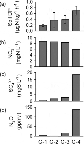
The riverbed EOS content at site No. 15 was relatively high at 254 mg kg^–1 (Figure 2(f)) and therefore the soil EOS and WESOC in a stream bank were vertically evaluated (Figure 6(a,b)). The vertical distribution of WESOC content was highest at the surface (333 mg kg^–1), intermediate at 50 cm, and reached a low constant value of about 80 mg kg^–1 at 75–200 cm. The EOS content was low and relatively constant from the surface to 160 cm but was extremely high (890 mg kg^–1) at 180–210 cm, which was near the stream water table (Figure 6(a)). At the EOS rich layer (G-4) in subsoil, higher soil DP was detected (Figure 7(a)). NO₃⁻ reduction, higher SO₄^2- and N₂O concentration were also detected in G-4 soil (Figure 7(b,c,d)).

Figure 6. (a) the photograph of stream bank at sample site No.15 where the riverbed EOS content was high. (b) vertical distribution of water-extractable soil organic carbon (WESOC) and easily oxidizable sulfur (EOS) contents in a stream bank at sample site No. 15. G-1, G-2, G-3, and G-4 represent the sample evaluated soil denitrification potential (DP) in.Figure 7

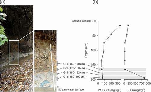
Figure 7. Results of (a) soil denitrification potentials (n = 3) in a stream bank at sample site No. 15. G-1, G-2, G-3, and G-4 indicate soil samples shown in Figure 6. Results of another incubation were also shown in (b) NO₃⁻ and (c) SO₄^2- concentrations in the solution, (d) N₂O concentration in the gas phase in the incubation bottle. Another incubation was conducted 15 g soil with 10 mg N L⁻¹ NO₃⁻ solution (50 mL) for 30 days (n = 1). The results in (b), (c) and (d) show the values after the 30 days incubation started

4. Discussion

4.1. Effects of catchment topography on in-stream NO₃ ^– concentrations

Our study revealed that stream NO₃ ^– concentrations spatially varied 8.1 times between the minimum and the maximum among catchments (Figure 2(a), Table 2). This result indicated that N retention or gaseous N loss in response to atmospheric N deposition varied largely among the catchments if assuming the atmospheric N deposition was same in each catchment. TWI or catchment slope were the most important factors controlling the spatial variation of in-stream NO₃ ^– concentrations (Figure 3(a), Tables 1 and 3). Based on the values of the absolute estimate values resulted by model 1 (Table 3) multiplied with the median value of the explanatory variables (Table 2), the magnitude of median TWI to the variation of predicted in-stream NO₃⁻ concentration was largest compared to other selected variables. Some researchers also reported in-stream NO₃⁻ was negatively correlated with TWI (Ogawa et al. 2006) and was positively correlated with slope (D’Arcy and Carignan 1997). Rinderer, Van Meerveld, and Seibert (2014) revealed TWI was a useful predictor of groundwater levels in catchments when groundwater levels change slowly (e.g., base flow or after rainfall events). Since our monitoring was conducted during base flow conditions, the groundwater levels in the catchments can be regarded as consistent with TWI variations. Therefore, we assumed the catchments with higher TWI had shallow groundwater table within catchments.

Catchment topography can control gaseous N loss such as denitrification by controlling water flows and groundwater table in the catchment. At sites as riparian zone with relatively flat topography increases the low hydraulic gradient, the water residence time, and the persistence of the anaerobic conditions necessary for denitrification (Vidon and Hill 2004). The significant positive correlations between slope and water velocity (r = 0.395, P < 0.05, Table S3) and the negative correlations between TWI and slope (r = −0.586, P < 0.01, Table S3) suggests that the gentle slope catchments have a longer water residence time and a higher soil moisture condition by the shallow groundwater level. In some catchments with relatively higher TWI, NO₃⁻ concentrations in the stream water were clearly lower than the water-weighted mean DIN concentration (0.32 mg N L⁻¹) in the atmospheric deposition as the N input to the catchment (Figure 3(a)). Therefore, the catchments with lower NO₃ ^– concentration in stream water would be a result of enhanced denitrification by in those catchments, which in turn resulted from the lower hydraulic gradients and greater abundance of anaerobic conditions associated with a gentle slope and high TWI. On the other hand, in the steep slope catchments, the relatively lower groundwater level and faster drainage might have lost the chance for denitrification and maintain a higher NO₃⁻ concentration. Schiff et al. (2002) reported the ten-fold difference in N export from surface water between adjacent two catchments resulted from a difference in slope which controlled water table dynamics and the lower NO₃⁻ concentration in the gentle slope catchments.

The trend of negative relationships between slope and dN₂O concentration (r = −0.411, P < 0.05), and NO₃⁻ and dN₂O (r = −0.232, P = 0.193) (Table S3) suggested that denitrification was likely enhanced in the catchments with gentle slope because N₂O is an intermediate product of the denitrification process (Tiedje 1994). Although N₂O can be produced by both nitrification and denitrification, Osaka et al. (2006) reported that much N₂O was produced in the groundwater system at the foot of the slope mainly through denitrifcaion and was transported by groundwater flow in a forest catchment. The results of the soil incubation in Figure 7 also indicated that N₂O in the subsoil (G-4) could be produced mainly by denitrification because both higher soil DP and NO₃⁻ reduction were observed. In a gentle slope and high TWI catchment with shallow groundwater, denitrification may promote N₂O and it could be transported by groundwater flow to the stream in a dissolved form. But the correlations between in-stream NO₃⁻, TWI and dN₂O were not so clear likely because N₂O production also depends on NO₃⁻ concentration (Osaka et al. 2006) and can be finally reduced to N₂ by denitrification under anoxic condition.

Another possible reason for the low NO₃⁻ concentration in the high TWI catchments would be N uptake by plant which was considered as a major N retention process in catchments. Plant may uptake more N by accessing NO₃⁻ easily around root zone likely because of a shallow water table by higher TWI. Foliar N concentration can increase where catchment N retention by the plant is high in response to atmospheric N deposition (Lovett and Goodale 2011). Therefore, foliar N concentration may increase in the catchments with higher TWI, if plant N retention was a major reason for the lower in-stream NO₃⁻ concentration. However, no significant correlations were found between foliar N concentration of Japanese cedar trees at the riparian forest in each catchment and TWI, and in-stream NO₃⁻ concentration (see Fig. S3). In a comparative study of two adjacent catchments with same atmospheric N deposition but N export considerably different by a factor of 17, higher foliar N concentration was observed rather in the catchment with higher N export (Makino et al. 2017). Although there were many uncertainties regarding N uptake by plants in the catchments such as tree age, tree species, planting, and density, as far as judging by foliar N concentration of Japanese cedar which was the representative plant in the catchments, N retention by plant uptake might not be an important factor to keep in-stream NO₃⁻ concentration low in the high TWI catchments.

The topographic analysis of the present study using mean NO₃ ^– data was not designed to explain temporal dynamics of in-stream NO₃ ^– concentration. However, Duncan, Groffman, and Band (2013) reported that topography was a much stronger controller of oxygen, and thus denitrification, as compared to rainfall, which had little influence on temporal variation in oxygen concentration in the soil air. Our finding that slope and TWI were significantly related with NO₃⁻ in seven and five of the nine sampling times, respectively (Table 1) also supported the notion that topography is a strong controller of spatial variation in-stream NO₃ ^– concentration with less seasonal dependence.

pTWI was also selected the explanatory variable for in-stream NO₃⁻ concentration (Table 2). Since pTWI is the TWI of each cell on the water sampled point, this result suggested that microtopography near water-sampled point also could affect in-stream NO₃⁻ concentration in the catchment. But the magnitude of microtopography (pTWI) on the variation of the predicted in-stream NO₃⁻ concentration by model 1 would not be so large compared to that of catchment scale topography (TWI) when comparing the value of the absolute value of the estimate (Table 3) multiplied with a median value of the explanatory variables (Table 2). The value of pTWI (1.58) was only one-fifth of the value of median TWI (7.8).

Slope aspect will control soil N processes other than denitrification through soil microorganisms and vegetation, primarily by receiving in variable net solar radiation on the slope, which may cause the spatial variation of in-stream NO₃⁻ concentration. In the northern hemisphere, net solar radiation can be generally higher on south-facing than on north-facing slopes. The results of the GLM showed both slope aspect_EW and slope aspect_NS were selected as explanatory variables for in-stream NO₃⁻ concentration (Table 2). The estimate sign indicated that in-stream NO₃⁻ concentration was lower in the east- and the south-facing slope catchments. Peterjohn et al. (1999) reported that the soil on the south-facing slope had a lower NO₃⁻ content, lower net nitrification rate, and lower NO₃⁻ concentration in leaching water compared to the east-facing slope. Kong et al. (2019) reported that soil mineral N and net N mineralization rate were significantly higher on the east-facing slope than on the west-facing slope, and were controlled by soil moisture. Gilliam et al. (2014) found that in addition to soil mineral N content and net nitrification rates, the microbial and the plant communities also markedly differed between the northeast- and the southwest-facing slopes. In these study data sets, it is difficult to discuss which processes controlled soil N in the catchments having different slope aspects, but GLM results suggested that the catchment slope aspects may control stream N concentration likely by regulating soil N processes other than denitrification such as mineralization, nitrification, and plant N uptake. The magnitude of slope aspect on the variation of the predicted in-stream NO₃⁻ concentration by model 1 would not be so large compared to that of median TWI (at least less than one-fifth of the TWI) when considering the value of the absolute value of the estimate (Table 3), and the median value and the range of the explanatory variables (Table 2).

4.2. Possibility of sulfur denitrification and subsoil denitrification in the LHW

Generally, most NO₃ ^– is reduced by denitrifying heterotrophs rather than by chemoautotrophs such as sulfur-oxidizing bacteria because NO₃ ^– reduction by organic matter should thermodynamically precede reduction by sulfide such as pyrite (Postma et al. 1991). Previous studies have reported that when the reactive organic C was sufficiently low to serve as an electron donor for denitrification, pyrite was considered the main electron donor in subsurface layers (Baker et al. 2012; Postma et al. 1991). In the Jurassic Lincolnshire limestone, Baker et al. (2012) suggested that pyrite was the main electron donor since no significant decrease in organic C content was found likely because of hardly decomposable organic C could not be used by heterotrophic microbes in the old sediments. The distribution of EOS was spatially and vertically independent of WESOC (Figure 2(e,f), Figure 6) in this study site. Although EOS content in the riverbed sediments was not selected in the GLM analysis as an explanatory variable for the prediction of in-stream NO₃ ^– concentration (Table 3), the significant positive relationship between EOS content and in-stream SO₄^{2 –} concentration, and the trend of NO₃⁻ decrease with EOS (Figure 5(a,b)) possibly suggested sulfur-mediated denitrification had occurred somewhere else. For example, at site No. 15, the EOS at the G-4 layer (180–200 cm) was a likely source of electron donors for sulfur denitrification in the soils (Figure 6). Actually, larger NO₃⁻ reduction with increasing N₂O and SO₄^2- concentrations, and higher soil DP were detected in the G-4 layer (Figure 7). In addition, sulfur-oxidizing bacteria that have the ability of NO₃⁻ reduction (Thiobacillus denitrificans) was also detected in the soil (see Fig. S2). These results suggested sulfur denitrification can occur in the subsoil because of the existence of potential electron donor for denitrification, possibly resulting in reduce NO₃⁻ especially in the soils with the high TWI catchments accompanied with anaerobic conditions by shallow groundwater.

The origin of EOS in the LHW may be sulfides that were deposited when the LHW was a marine environment (Shiraishi and Matoba 1992). Some of the high EOS detected in riverbed sediments will be derived from sulfide-rich layers such as the G-4 layer near the stream-water surface (Figure 6) due to an erosion of stream banks during flooding. The sites with higher EOS content in riverbed sediments and similar characteristics to No. 15 such as site No.14, 16, 17, and 19 (Figure 2(f)) might have a high EOS layer like the G-4 within catchments. This study suggested EOS in riverbed sediments can contain site-specific information about denitrification hot spots driven by sulfides such as the G-4 layer. We need to obtain hydrogeological and bacterial evidences in more detail of sulfur denitrification in subsoil and sediment at sulfide-rich sites in the natural headwater catchment in the LHW.

4.3. Effect of sediment denitrification on in-stream NO₃ ^– concentration and its controlling factors

Riverbed sediments can remove in-stream NO₃ ^– as hot spots of denitrification in ecosystems (Seitzinger et al. 2006). Sediment DP was also selected as the predictor of variation in in-stream NO₃ ^– concentration in the LHW (Table 3) and negatively correlated with in-stream NO₃ ^– concentration (Figure 4(a)), although its magnitude to the variation of predicted in-stream NO₃⁻ would be small compared to other factors (Table 3, model 1). The GLM analysis of factors potentially related to DP showed that the greater contributors to variation were water velocity and the WESOC contents of sediment (Table 3, models 2 and 3). Previous studies have reported that the DP of riverbed sediment was strongly correlated with organic matter content in the sediment (Inwood, Tank, and Bernot 2007) and in-stream DOC concentration (Findlay et al. 2011), likely because organic C is the predominant electron donor for denitrifying heterotrophs. In the present study, the WESOC content of sediment also contributed to the variation in sediment DP (Table 3, Figure 4(c)). Water velocity would have controlled the sediment texture, which are important factors for denitrification (Groffman and Tiedje 1989; Ullah and Faulkner 2006). Faster water velocity can sweep WESOC in the bottom sediments. Because water velocity and WESOC were controlled by topography (slope and TWI) (Figure 3(d,e), and Table S2), topography would have also indirectly affected sediment DP. Positive relationship between median TWI and sediment WESOC (Figure 3(e)) suggested that WESOC was accumulated in the catchments with higher TWI. Soils with higher moisture content delay organic matter decomposition and can increase SOM (soil organic matter) (Davidson, Belk, and Boone 1998; Brady and Weil 2008). Some studies have revealed that TWI was a good predictor for the distribution of soil carbon or SOM in landscape (Sumfleth and Duttmann 2008; Liu et al. 2015). This study showed that median TWI in catchments was also a good indicator of riverbed WESOC content that can be an electron donor for denitrification.

Latitude was the better predictor of sediment DP (Table 3), and it might include other factors driving N cycle as an explanatory variable. For example, the strong negative correlation between latitude and elevation (r = −0.597, P < 0.01) and slope (r = −0.658, P < 0.01) indicated that latitude might include the effects of elevation (e.g., temperature) and slope or both indirectly on the N cycle. When GLM analysis was performed except latitude from the sediment DP prediction model, dN₂O was selected instead of latitude (Table 3, model 3). dN₂O also correlated with latitude (r = 0.640, P < 0.01), elevation (r = −0.445, P < 0.01), and slope (r = −0.411, P < 0.01), significantly (Table S3). It may imply that topographical factors and N₂O production process in catchments, and their interactions are related to sediments DP.

4.4. Implications and limitations for ecosystem-wide denitrification and stream NO₃⁻ concentration

This study demonstrated that topography and the distribution of electron donors for denitrification in headwater catchments explained much of the spatial variation in in-stream NO₃ ^– concentration in the LHW. An assumption underlying the hypothesis of the present study was that riverbed sediments, which have been used to identify water quality (Horowitz and Elrick 2017), are representative of the abundance and activity of electron donors for denitrification at the catchment scale. The results partly supported this assumption in that the WESOC of the riverbed sediment samples were selected in the GLM analysis as predictors for sediment DPs.

Although EOS content in the riverbed sediments was not selected as a significant explanatory variable for the prediction of in-stream NO₃ ^– concentration, the focus on sulfide minerals to elucidate the NO₃ ^– removal process in natural ecosystems will be important in regions facing the Japan Sea such as the LHW because their past geological history confers them with high contents of sulfide minerals and because they also receive high N deposition rates, especially from East Asia (Tomoyose et al. 2009). Furthermore, the middle and downstream reaches of LHW and the area inside the polder, which had been a marine and a brackish environment (Shiraishi 1990), are expected to contain high levels of sulfides in soils and sediments because (iron) sulfides are generally produced in marine systems (Richkard and Luther 2007) and to receive even greater anthropogenic N inputs from agriculture, providing an even stronger linkage between the N cycle and sulfur. Molecular biological analysis is needed to elucidate the bacterial communities in the environment to further understand the distribution and strength of sulfur denitrification in the LHW.

5. Conclusion

The present study demonstrated that catchment topography was the primary factor explaining the spatial variation of in-stream NO₃ ^– concentration in headwater catchments of the Lake Hachiro watershed (LHW). Topographic wetness index (TWI) in catchment negatively correlated with in-stream NO₃⁻ concentration and was the most important predictor of the variation of in-stream NO₃⁻ concentration. The one possible process behind it was denitrification in the catchment soil which would result from the lower hydraulic gradients and greater abundance of anaerobic conditions possibly associated with gentle slope and high TWI. Electron donors for denitrification such as WESOC and reduced S in riverbed sediments could help to explain sediment DP or site-specific subsoil DP driven by sulfide, respectively. This study demonstrated that topographic analysis (to understand the prevalence of anoxic conditions) combined with soil and geochemical data (to understand the relative abundance of electron donors available to drive denitrification) is important to predict the spatial distribution of stream NO₃⁻ concentrations and potential denitrification at watershed and ecosystem scales.

Disclosure statement

No potential conflict of interest was reported by the authors.

Supplementary material

Supplemental data for this article can be accessed here.

Additional information

Funding

This study was partly supported by a Grant-in-Aid for Young Scientists (B), 23780340, and Research (B), No.26281011 provided by Japan Society for the Promotion of Science (JSPS), and by the Strategic Japanese-Chinese Cooperative Program “Comparative study of nitrogen cycling and its impact on water quality in agricultural watersheds in Japan and China,” provided by JST-NSFC.

References

- Baker, K. M., S. H. Bottrell, D. Hatfield, R. J. G. Mortimer, R. J. Newton, N. E. Odling, and R. Raiswell. 2012. “Reactivity of Pyrite and Organic Carbon as Electron Donors for Biogeochemical Processes in the Fractured Jurassic Lincolnshire Limestone Aquifer, UK.” Chemical Geology 332–333: 26–31. doi:https://doi.org/10.1016/j.chemgeo.2012.07.029.
- Beven, K. 1997. “TOPMODEL: A Critique.” Hydrological Process 11: 1069–1085. doi:https://doi.org/10.1002/(SICI)1099-1085(199707)11:9<1069::AID-HYP545>3.0.CO;2-O.
- Beven, K. J., and M. J. Kirkby. 1979. “A Physically Based, Variable Contributing Area Model of Basin Hydrology.” Hydrological Sciences Bulletin 24: 43–69. doi:https://doi.org/10.1080/02626667909491834.
- Biodiversity Center of Japan, Nature Conservation Bureau, Ministry of the Environment. “National Survey on the Natural Environment, 6th and 7th Vegetation Survey.” Accessed 21 May 2009. http://www.vegetation.jp/index.html
- Boyer, E. W., R. W. Howarth, J. N. Galloway, F. J. Dentener, P. A. Green, and C. J. Vörösmarty. 2006. “Riverine Nitrogen Export from the Continents to the Coasts.” Global Biogeochemical Cyclcles 20: GB1S91. doi:https://doi.org/10.1029/2005GB002537.
- Brady, N. C., and R. R. Weil. 2008. “12 Soil Organic Matter.” In The Nature and Properties of SOILS, 495–541. 14th ed. Pearson.
- Brunet, R. C., and L. J. Garcia-Gil. 1996. “Sulfide-induced Dissimilatory Nitrate Reduction to Ammonia in Anaerobic Freshwater Sediments.” FEMS Microbiology Ecology 21: 131–138. doi:https://doi.org/10.1016/0168-6496(96)00051-7.
- Burgin, A. J., and S. K. Hamilton. 2008. “NO3–driven SO42- Production in Freshwater Ecosystems: Implications for N and S Cycling.” Ecosystems 11: 908–922. doi:https://doi.org/10.1007/s10021-008-9169-5.
- Carpenter, S., F. N. Caraco, D. L. Correll, R. W. Howarth, A. N. Sharple, and V. H. Smith. 1998. “Nonpoint Pollution of Surface Waters with Phosphorus and Nitrogen.” Ecological Applications 8: 559–568. doi:https://doi.org/10.1890/1051-0761(1998)008[0559:NPOSWW]2.0.CO;2.
- Core Team, R. 2018. “R: A Language and Environment for Statistical Computing. R Foundation for Statistical Computing.” Vienna, Austria. Accessed 1 March 2018. https://www.R-project.org/
- Craig, L., J. M. Bahr, and E. E. Roden. 2010. “Localized Zones of Denitrification in a Floodplain Aquifer in Southern Wisconsin, USA.” Hydrogeology Journal 18: 1867–1879. doi:https://doi.org/10.1007/s10040-010-0665-2.
- Craig, L. S., M. A. Palmer, D. C. Richardson, S. Filoso, E. S. Bernhardt, B. P. Bledsoe, M. W. Doyle, et al. 2008. “Stream Restoration Strategies for Reducing River Nitrogen Loads.” Frontiers in Ecology and the Environment 6:529–538. doi:https://doi.org/10.1890/070080.
- D’Arcy, P., and R. Carignan. 1997. “Influence of Catchment Topography on Water Chemistry in Southeastern Québec Shield Lakes.” Canadian Journal of Fisheries and Aquatic Sciences 54: 2215–2227. doi:https://doi.org/10.1139/f97-129.
- Davidson, E. A., E. Belk, and R. D. Boone. 1998. “Soil Water Content and Temperature as Independent or Confounded Factors Controlling Soil Respiration in a Temperate Mixed Hardwood Forest.” Global Change Biology 4: 217–227. doi:https://doi.org/10.1046/j.1365-2486.1998.00128.x.
- Duncan, J. M., P. M. Groffman, and L. E. Band. 2013. “Towards Closing the Watershed Nitrogen Budget: Spatial and Temporal Scaling of Denitrification.” Journal of Geophysical Research: Biogeosciences 118: 1105–1119. doi:https://doi.org/10.1002/jgrg.20090.
- Fang, Y., P. Gundersen, R. D. Vogt, K. Koba, F. Chen, X. Y. Chen, and M. Yoh. 2011. “Atmospheric Deposition and Leaching of Nitrogen in Chinese Forest Ecosystems.” Journal of Forest Research 16: 341–350. doi:https://doi.org/10.1007/s10310-011-0267-4.
- Findlay, S. E. G., P. J. Mulholland, S. K. Hamilton, J. L. Tank, M. J. Bernot, A. J. Burgin, C. L. Crenshaw, et al. 2011. “Cross-stream Comparison of Substrate-specific Denitrification Potential.” Biogeochemistry 104: 381–392. doi:https://doi.org/10.1007/s10533-010-9512-8.
- Florinsky, I. V., S. McMahon, and D. L. Burton. 2004. “Topographic Control of Soil Microbial Activity: A Case Study of Denitrifiers.” Geoderma 119: 33–53. doi:https://doi.org/10.1016/S0016-7061(03)00224-6.
- Galloway, J. N., and E. B. Cowling. 2002. “Reactive Nitrogen and the World: 200 Years of Change.” Ambio 31: 64–71. doi:https://doi.org/10.1579/0044-7447-31.2.64.
- Garcia-Gil, L. J., and H. L. Golterman. 1993. “Kinetics of FeS-mediated Denitrification in Sediments from the Camargue (Rhone Delta, Southern France).” FEMS Microbiology Ecology 13: 85–91. doi:https://doi.org/10.1016/0168-6496(93)90026-4.
- Geospatial Information Authority of Japan. Accessed July 6 2010. http://fgd.gsi.go.jp/download/
- Gilliam, F. S., R. Hédl, M. Chudomelová, R. L. McCulley, and J. A. Nelson. 2014. “Variation in Vegetation and Microbial Linkages with Slope Aspect in a Montane Temperate Hardwood Forest.” Ecosphere 5 (5): A66. doi:https://doi.org/10.1890/ES13-00379.1.
- Groffman, P. M., and J. M. Tiedje. 1989. “Denitrification in North Temperate Forest Soils: Relationships between Denitrification and Environmental Factors at the Landscape Scale.” Soil Biology and Biochemistry 21: 621–626. doi:https://doi.org/10.1016/0038-0717(89)90054-0.
- Groffman, P. M., K. Butterbach-Bahl, R. W. Fulweiler, A. J. Gold, J. L. Morse, E. K. Stander, C. Tague, et al. 2009. “Challenges to Incorporating Spatially and Temporally Explicit Phenomena (Hotspots and Hot Moments) in Denitrification Models.” Biogeochemistry 93 :49–77. doi:https://doi.org/10.1007/s10533-008-9277-5.
- Harms, T. K., and N. B. Grimm. 2008. “Hot Spots and Hot Moments of Carbon and Nitrogen Dynamics in a Semiarid Riparian Zone.” Journal of Geophysical Research 113: G01020. doi:https://doi.org/10.1029/2007JG000588.
- Hayakawa, A., K. P. Woli, M. Shimizu, K. Nomaru, K. Kuramochi, and R. Hatano. 2009. “Nitrogen Budget and Relationships with Riverine Nitrogen Exports from a Dairy Cattle Farming Catchment in Eastern Hokkaido, Japan.” Soil Science and Plant Nutrition 55: 800–819. doi:https://doi.org/10.1111/j.1747-0765.2009.00421.x.
- Hayakawa, A., M. Hatakeyama, R. Asano, Y. Ishikawa, and S. Hidaka. 2013. “Nitrate Reduction Coupled with Pyrite Oxidation in the Surface Sediments of a Sulfide-rich Ecosystem.” Journal of Geophysical Research: Biogeosciences 118: 639–649. doi:https://doi.org/10.1002/jgrg.20060.
- Hayakawa, A., M. Nakata, R. Jiang, K. Kuramochi, and R. Hatano. 2012. “Spatial Variation of Denitrification Potential of Grassland, Windbreak Forest, and Riparian Forest Soils in an Agricultural Catchment in Eastern Hokkaido, Japan.” Ecological Engineering 47: 92–100. doi:https://doi.org/10.1016/j.ecoleng.2012.06.034.
- Horowitz, A. J., and A. Elrick. 2017. “The Use of Bed Sediments in Water Quality Studies and Monitoring Programs.” Proceedings of the International Association of Hydrological Sciences 375: 11–17. doi:https://doi.org/10.5194/piahs-375-11-2017.
- Howarth, R. W., G. Billen, D. Swaney, A. Townsend, N. Jaworski, K. Lajtha, J. A. Downing, et al. 1996. “Regional Nitrogen Budgets and Riverine N and P Fluxes for the Drainages to the North Atlantic Ocean: Natural and Human Influences.” Biogeochemistry 35 :75–139. doi:https://doi.org/10.1007/BF02179825.
- Imai, N., S. Terashima, A. Ohta, M. Mikoshiba, T. Okai, Y. Tachibana, S. Togashi, et al. 2004. Geochemical Map of Japan. Tsukuba: Geological Survey of Japan, AIST.
- Inwood, S. E., J. L. Tank, and M. J. Bernot. 2007. “Factors Controlling Sediment Denitrification in Midwestern Streams of Varying Land Use.” Microbial Ecology 53: 247–258. doi:https://doi.org/10.1007/s00248-006-9104-2.
- Japan Meteorological Agency. 2013. “Information of Meteorological Statistics.” Accessed April 19 2013. http://www.data.jma.go.jp/obd/stats/etrn/index.php
- Jørgensen, C. J., C. S. Jacobsen, B. Elberling, and J. Aamand. 2009. “Microbial Oxidation of Pyrite Coupled to Nitrate Reduction in Anoxic Groundwater Sediment.” Environmental Science Technology 43: 4851–4857. doi:https://doi.org/10.1021/es803417s.
- Kimura, S. D., X. Yan, R. Hatano, A. Hayakawa, K. Kohyama, C. Ti, K. Kuramochi, Z. Cai, and M. Saito. 2012. “Influence of Agricultural Activity on Nitrogen Budget in Chinese and Japanese Watersheds.” Pedosphere 22: 137–151. doi:https://doi.org/10.1016/S1002-0160(12)60001-0.
- Kondo, T. 2010. “Changes and Problems of Hydrological and Environmental Characteristic of Lake Hachiro.” Journal of Japan Society on Water Environment 33: 292–298. in Japanese.
- Kong, W., Y. Yao, Z. Zhao, X. Qin, H. Zhu, X. Wei, M. Shao, Z. Wang, K. Bao, and M. Su. 2019. “Effects of Vegetation and Slope Aspect on Soil Nitrogen Mineralization during the Growing Season in Sloping Lands of the Loess Plateau.” Catena 172: 753–763. doi:https://doi.org/10.1016/j.catena.2018.09.037.
- Korom, S. F. 1992. “Denitrification in the Saturated Zone: A Review.” Water Resources Research 28: 1657–1668. doi:https://doi.org/10.1029/92WR00252.
- Liu, S., N. An, J. Yang, S. Dong, C. Wang, and Y. Yin. 2015. “Prediction of Soil Organic Matter Variability Associated with Different Land Use Types in Mountainous Landscape in Southwestern Yunnan Province, China.” Catena 133: 137–144. doi:https://doi.org/10.1016/j.catena.2015.05.010.
- Lovett, G. M., and C. L. Goodale. 2011. “A New Conceptual Model of Nitrogen Saturation Based on Experimental Nitrogen Addition to an Oak Forest.” Ecosystems 14: 615–631. doi:https://doi.org/10.1007/s10021-011-9432-z.
- Makino, S., N. Tokuchi, K. Fukushima, and T. Kawakami. 2017. “Nitrogen Dynamics of Nitrogen Saturated and Unsaturated Deciduous Forest Ecosystems on Toyama Plain, Japan.” Journal of the Japanese Forest Society 99: 120–128. doi:https://doi.org/10.4005/jjfs.99.120.
- McGrigal, K. 2018. “Analysis of Environmental Data Conceptual Foundations: Data Exploration, Screening & Adjustments.” University of Massachusetts Amherst. Accessed 30 November 2018. https://www.umass.edu/landeco/teaching/ecodata/schedule/ecodata_schedule.html
- Minamikawa, K., A. Hayakawa, S. Nishimura, H. Akiyama, and K. Yagi. 2011. “Comparison of Indirect Nitrous Oxide Emission through Lysimeter Drainage between an Andosol Upland Field and a Fluvisol Paddy Field.” Soil Science and Plant Nutrition 57: 843–854. doi:https://doi.org/10.1080/00380768.2011.635427.
- Murano, H., T. Yamanaka, and C. Mizota. 2000. “Origin of Sulfides and Associated Sulfates in Neogene Sediments along the Kitakami River Basin from Northeast Japan—Sulfur Isotopic Characterization and Implications for Land Consolidation.” Pedologist 44: 81–90. in Japanese with English summary.
- Ogata-mura village office. “History.” Accessed March 17 2014. http://www.ogata.or.jp/encyclopedia/history/2-2.html (in Japanese).
- Ogawa, A., H. Shibata, K. Suzuki, M. J. Mitchell, and Y. Ikegami. 2006. “Relationship of Topography to Surface Water Chemistry with Particular Focus on Nitrogen and Organic Carbon Solutes within a Forested Watershed in Hokkaido, Japan.” Hydrological Processes 20: 251–265. doi:https://doi.org/10.1002/hyp.5901.
- Osaka, K., N. Ohte, K. Koba, M. Katsuyama, and T. Nakajima. 2006. “Hydrologic Controls on Nitrous Oxide Production and Consumption in a Forested Headwater Catchment in Central Japan.” Journal of Geophysical Research 111 (G1): G01013. doi:https://doi.org/10.1029/2005JG000026.
- Peterjohn, W. T., C. J. Foster, M. J. Christ, and M. B. Adams. 1999. “Patterns of Nitrogen Availability within a Forested Watershed Exhibiting Symptoms of Nitrogen Saturation.” Forest Ecology and Management 119 (1–3): 247–257. doi:https://doi.org/10.1016/S0378-1127(98)00526-X.
- Postma, D., C. Boesen, H. Kristiansen, and F. Larsen. 1991. “Nitrate Reduction in an Unconfined Sandy Aquifer: Water Chemistry, Reduction Processes, and Geochemical Modeling.” Water Resources Research 27: 2027–2045. doi:https://doi.org/10.1029/91WR00989.
- Quinn, P. F., K. J. Beven, and R. Lamb. 1995. “The ln(α/tanβ) Index: How to Calculate It and How to Use It within the Topmodel Framework.” Hydrological Processes 9: 161–182. doi:https://doi.org/10.1002/hyp.3360090204.
- Richkard, D., and G. W. Luther III. 2007. “Chemistry of Iron Sulfides.” Chemical Reviews 107: 514–562. doi:https://doi.org/10.1021/cr0503658.
- Rinderer, M., H. J. Van Meerveld, and J. Seibert. 2014. “Topographic Controls on Shallow Groundwater Levels in a Steep, Prealpine Catchment: When are the TWI Assumptions Valid?” Water Resources Research 50: 6067–6080. doi:https://doi.org/10.1002/2013WR015009.
- Sasaki, J. 2010. “Water Quality Conservation Measures of Lake Hachiro.” Journal of Japanese Society of Water Environment 33: 287–291. in Japanese.
- Sawamoto, T., K. Kusa, R. Hu, and R. Hatano. 2003. “Dissolved N2O, CH4, and CO2 Emissions from Subsurface-drainage in a Structured Clay Soil Cultivated with Onion in Central Hokkaido, Japan.” Soil Science and Plant Nutrition 49: 31–38. doi:https://doi.org/10.1080/00380768.2003.10409976.
- Schiff, S. L., K. J. Devito, R. J. Elgood, P. M. McCrindle, J. Spoelstra, and P. Dillon. 2002. “Two Adjacent Forested Catchments: Dramatically Different NO3− Export.” Water Resources Research 38: 281–2813. doi:https://doi.org/10.1029/2000WR000170.
- Schwientek, M., F. Einsiedl, W. Stichler, A. Stogbauer, H. Strauss, and P. Maloszewski. 2008. “Evidence for Denitrification Regulated by Pyrite Oxidation in a Heterogeneous Porous Groundwater System.” Chemical Geology 255: 60–67. doi:https://doi.org/10.1016/j.chemgeo.2008.06.005.
- Seitzinger, S., J. A. Harrison, J. K. Böhlke, A. F. Bouwman, R. Lowrance, B. Peterson, C. Tobias, and G. Van Drecht. 2006. “Denitrification across Landscapes and Waterscapes: A Synthesis.” Ecological Applications 16: 2064–2090. doi:https://doi.org/10.1890/1051-0761(2006)016[2064:DALAWA]2.0.CO;2.
- Shiraishi, T. 1990. “Holocene Geologic Development of the Hachiro-gata Lagoon, Akita Prefecture, Northeast Honshu, Japan.” Memoirs of the Geological Society of Japan 36: 47–69. in Japanese with English summary.
- Shiraishi, T., and Y. Matoba. 1992. “Neogene Paleogeography and Paleoenvironment in Akita and Yamagata Prefectures, Japan Sea Side of Northeast Honshu, Japan.” Memoirs of the Geological Society of Japan 37: 39–51. in Japanese with English summary.
- Straub, K. L., M. Benz, B. Schlik, and F. Widdel. 1996. “Anaerobic, Nitrate-dependent Microbial Oxidation of Ferrous Iron.” Applied Environmental Microbiology 62: 1458–1460. doi:https://doi.org/10.1128/AEM.62.4.1458-1460.1996.
- Sumfleth, K., and R. Duttmann. 2008. “Prediction of Soil Property Distribution in Paddy Soil Landscapes Using Terrain Data and Satellite Information as Indicators.” Ecological Indicators 8 (5): 485–501. doi:https://doi.org/10.1016/j.ecolind.2007.05.005.
- Tiedje, J. M. 1994. “Denitrifiers.” In Methods of Soil Analysis. Part 2. SSSA Book Ser. 5, edited by R. W. Weaver, et al., 245–257. Madison: Soil Science Society of America.
- Tomoyose, N., I. Noguchi, T. Ohizumi, Y. Kitamura, F. Nakagawa, T. Mizoguchi, K. Murano, and H. Mukai. 2009. “Studies on Trans-boundary Air Pollution in View of Wet Deposition Data (FY2003–FY2006) Monitored in the Survey by Japan Environmental Laboratories Association.” Journal of Japan Society of Atmospheric Environment 44: 361–381. in Japanese with English summary.
- Torrentó, C., J. Cama, J. Urmeneta, N. Otero, and A. Soler. 2010. “Denitrification of Groundwater with Pyrite and Thiobacillus Denitrificans.” Chemical Geology 278: 80–91. doi:https://doi.org/10.1016/j.chemgeo.2010.09.003.
- Torrentó, C., J. Urmeneta, N. Otero, A. Soler, M. Vinas, and J. Cama. 2011. “Enhanced Denitrification in Groundwater and Sediments from a Nitrate-contaminated Aquifer after Addition of Pyrite.” Chemical Geology 287: 90–101. doi:https://doi.org/10.1016/j.chemgeo.2011.06.002.
- Ullah, S., and S. P. Faulkner. 2006. “Denitrification Potential of Different Land-use Types in an Agricultural Watershed, Lower Mississippi Valley.” Ecological Engineering 28: 131–140. doi:https://doi.org/10.1016/j.ecoleng.2006.05.007.
- Vidon, P., and A. R. Hill. 2004. “Denitrification and Patterns of Electron Donors and Acceptors in Eight Riparian Zones with Contrasting Hydrogeology.” Biogeochemistry 71: 259–283. doi:https://doi.org/10.1007/s10533-004-9684-1.
- Vitousek, P. M., H. A. Mooney, J. Lubchenco, and J. M. Melillo. 1997. “Human Domination of Earth’s Ecosystems.” Science 277: 494–499. doi:https://doi.org/10.1126/science.277.5325.494.
- Yang, X., S. Huang, Q. Wu, and R. Zhang. 2012. “Nitrate Reduction Coupled with Microbial Oxidation of Sulfide in River Sediment.” Journal of Soils and Sediments 12: 1435–1444. doi:https://doi.org/10.1007/s11368-012-0542-9.