Critical reevaluation of an efficient sampling design for assessing soil properties using bootstrap sampling and geostatistical analysis in Japanese large-scale paddy fields

ABSTRACT

Soil test is a key step toward providing recommendations for better crop management. Several soil samples have been traditionally assumed to be sufficient for soil tests to represent field-specific values in conventional Japanese small-scale paddy fields. However, rethinking soil sampling design is required, as many small-scale (<0.3 ha) paddy fields have been consolidated into large-scale (>1 ha) paddy fields to enhance the efficiency of crop production. The purpose of this study is to explore an efficient soil sampling design, including sample size for representing field-specific values and sampling distance for representing spatial variations, in central Japan using bootstrap sampling and geostatistical analysis. Fourteen soil properties were quantified from 553 samples, which was collected at a distance of 24.4 m on average in large-scale paddy fields with continuous rice cultivation and rotation of rice and upland crops (winter wheat and soybean). The results show that the conventional sampling size (n = 3 for each field) achieved mean estimation within 10% error with 95% confidence intervals only for pH and sand content in almost all fields; thus, an optimization of field-specific uniform liming rate is recommended for reducing cost. Geostatistical analysis shows that the recommended soil sampling distance should be 15–163 m, depending on specific soil properties. The results further show that it was difficult to obtain reliable estimates of exchangeable K and mineralizable N because of the high level of spatial uncertainty with high nugget variance. Thus, practitioners should note that the outcomes from soil tests inherently included fine-scale errors in available nutrient levels which may preclude rationale prescriptions. This study demonstrated that appropriate soil sampling design and the subsequent soil management can differ depending on specific soil properties in the actual farming scale of large-scale paddy fields.

KEY WORDS:

• Geostatistical analysis
• paddy fields
• sample size
• sampling distance
• spatial variability
• soil properties

1. Introduction

Soil physical, hydrological, chemical, and biological features are key knowledge for understanding the relationships between soil and crops, especially in precision agriculture, environmental management, and crop growth modeling (Bhakta, Phadikar, and Majumder 2019). Due to the comprehensive influence of various physical, chemical, and biological reactions at various intensities and scales, soil shows a high degree of spatial variability (Goovaerts 1999). Changes in soil measurements and processes in turn affect plant growth and the environment (Tomasi et al. 2014; Pii, Cesco, and Mimmo 2015). Thus, accurate soil tests are required to optimize agricultural inputs.

Soil sampling is fundamental for soil quality assessment because it greatly affects the measurement precision representing field-specific features and spatial variability across fields. Therefore, sampling approaches have presented a controversial topic for agronomy and soil science. Fundamentally, there are two types of spatial sampling theories: design-based approaches based on random sampling and model-based approaches based on geostatistics (De Gruijter and Ter Braak 1990; Brus 2021). A design-based approach is often referred to as classical sampling theory to represent population parameters (e.g., mean and variance). A model-based approach that takes spatial autocorrelation into account can spatially interpolate the soil variables. Note that the variability of a soil test is affected by the spatial heterogeneity of the soil and the measurement accuracy. The aim of the survey strongly affects the choice of the statistical approaches (Brus and De Gruijter 1997). The design-based approach provides target quantities including totals, means, medians, or quartile in a certain field or region, while the model-based approach predicts values at points that are very informative when implementing variable-rate application (VRA) technologies. Soil testing based on an inappropriate sampling approach may lead to unreliable or inaccurate diagnosis for crop management, even if the soil analysis features a high measurement accuracy (Jianwei 2019; Tan 2005). Due to resource and time constraints, it is not practical to collect tens or hundreds of soil samples from a single field. Therefore, in the actual sampling design process, the number of samples is always determined arbitrarily and does not follow statistical standards (Carré et al. 2007; Carter and Gregorich 2007).

To improve the efficiency of crop agricultural production in Japan, scattered small-scale paddy fields have been increasingly consolidated into large-scale paddy fields. Until the 1990s, approximately 55% of all fields were successfully consolidated into approximately 0.3 ha per field (Sato 2001). Currently, the Japanese government is offering further subsidies to promote consolidation of these 0.3-ha fields into large-scale fields exceeding 1.0 ha in area. Spatial variability in soil properties will become nonnegligible in large-scale fields, because crop establishment and yield could fluctuate within a field (Tanaka, Kono, and Matsui 2019; Zhou et al. 2022). In the traditional soil sampling method, usually 3–5 soil samples are collected in a single plot or field. In a small research area, the traditional soil sampling method may be sufficient to characterize the overall situation in the field, but this is not the case in a larger field. Furthermore, land use changes could alter the spatial heterogeneity of soil properties, which would greatly affect sample sizes required for estimating soil properties with prescribed precision (Li et al. 2010). In most practical situations, agronomists and crop advisors usually apply the traditional sampling approach, namely, design-based approach, which would preclude effective soil diagnosis. Extensive research efforts have attempted to evaluate spatial variability in soil properties based on model-based approach to develop site-specific management approaches and management zone delineations in large upland fields, primarily in Europe and the US (López-Granados et al. 2005; Mzuku et al. 2005). Although pilot-scale geostatistical analysis on soil properties in small-scale experimental paddy fields has been performed in Japan (Moritsuka et al. 2004; Yanai et al. 2000, 2001), knowledge about the spatial heterogeneity of large-scale paddy fields remains limited. Therefore, the validity of traditional soil sampling is questionable. To obtain representative soil samples, considering the economic cost and field variability according to the objectives of survey, it is very important to examine the measurement accuracy and the spatial variability of soil properties, which would permit more effective management practices.

The objective of this study is to examine the appropriate soil sampling approach in large-scale consolidated paddy fields. Given that the traditional soil sampling approach is used, field-specific soil assessment accuracy as affected by sample size was analyzed using the bootstrap method. Bootstrap method provides statistical inferences of standard errors, bias estimates, confidence intervals, and hypothesis tests without assumptions such as normal distributions or equal variances using resampling techniques (Hesterberg 2011), which is effective for limited data set. Stefano, Ferro, and Porto (2000) tested the performance of the bootstrap method in the estimation of the reference level of ¹³⁷Cs in an uneroded field and found that the bootstrap method can be used to generate a reliable estimated mean value and sample size even in a field where a small number of samples are taken. Spatial variability in soil properties and its uncertainty were further investigated using geostatistical analysis to assess the appropriate sampling distance and the potential application context of soil maps in Japanese large-scale consolidated paddy fields. The bootstrap method corresponds to field-specific soil management, and geostatistical analysis corresponds to site-specific management implemented by precision agriculture technology. Therefore, this study ultimately aimed to explore an appropriate soil management associated with sampling design.

2. Materials and methods

2.1. Study area

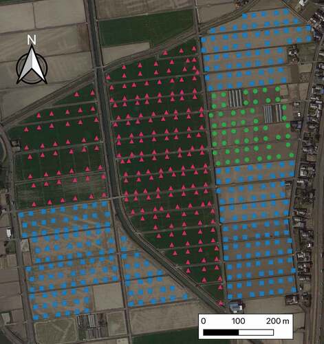
The study area is located in Kaizu, Gifu, Japan (35°11’ N, 136°40’ E; Figure 1), with an area of approximately 0.64 km² with 43 fields (Figure 1). The sampling area was much larger than previous studies (Moritsuka et al. 2004; Yanai et al. 2000, 2001) (e.g., 0.5 ha) investigating spatial variability of soil properties in an experimental paddy field; thus, we assumed that more robust and practical outcomes can be obtained. The climate is classified as warm and temperate. The average annual temperature is 14.2°C. Annual precipitation is 1907 mm. The soil texture is basically a sandy loam. The soil in the test area was classified as Entisols. There was only a 0–2 m elevation difference across the fields. Two planting systems were implemented in test area: (1) paddy rice only (6 fields) and (2) block rotation of three crops (paddy rice–winter wheat–soybean) over two years (37 fields). These two types of systems are commonly used in many parts of Japan. The frequent transition between paddy and upland fields may affect soil chemical properties. Each field’s planting system has remained the same for more than 10 years. Small-scale paddy fields with areas of approximately 0.3 ha were consolidated into large-scale paddy fields of approximately 1 ha in area in 1990s. There were originally 421 fields before the consolidations in 1980s. Therefore, this region was selected to investigate whether the types of cropping rotation affect the spatial variability of soil variables in large-scale paddy fields.

Figure 1. Soil sampling scheme.

The soil sampling points are shown as symbols in Figure 1. Green circles represent fields where only rice is planted (rice only). Red triangles and blue squares represent blocks 1 and 2 of crop rotation (paddy rice–winter wheat–soybean), respectively. Soil samples were collected in block 1 just after rice harvesting and in block 2 just after soybean harvesting.

2.2. Soil analysis

A total of 553 soil samples from 2019 to 2020 were analyzed in this study. The sampling distance ranged from 12 to 40 m (24.4 m on average). Because there were three crops in the rotation, soil sample collection occurred two times. After rice harvesting (16 October 2019), 342 soil samples were collected (green circles and blue squares in Figure 1). After soybean harvesting (27 February 2020), 211 soil samples were collected (red triangles in Figure 1). The surface soil (0–15 cm) was collected. At each location, three randomly located partial soil samples weighing approximately 0.5 kg were collected within one square meter and mixed to produce one composite sample. Soil samples were air-dried and sieved through 2.0-mm mesh before chemical analysis. It was impossible to collect soil samples from the different cropping systems at the same time because there was still a crop growing in another block. The approach taking temporal variations of soil properties derived from the different timings of sample collection into account was described in section 2.3.2.

Soil pH, electrical conductivity (EC), total carbon (TC), and nitrogen (TN) contents, particle size distribution (sand, silt, and clay), mineralizable N, available phosphorus (P), cation exchange capacity (CEC), exchangeable calcium (Ca), exchangeable magnesium (Mg), and exchangeable potassium (K) were measured. The particle size distribution was measured using the pipette method and sieving (Gee and Bauder, 1986). Total C and N were determined using a CN analyzer (Sumigraph NC-TR22, Sumitomo Chemical Co., Tokyo, Japan). Mineralizable N was determined according to the method of Inoko (1986). Briefly, soils were anaerobically incubated at 30°C for four weeks, and inorganic N was extracted with 2 mol L⁻¹ KCl solution. The concentrations of NH₄⁺ and NO₃⁻ in the extracts were then determined using the indophenol method (Keeney and Nelson 1983) and the Cataldo method (Cataldo et al. 1975), respectively. Mineralizable N was calculated by balancing the inorganic N (NH₄⁺ and NO₃⁻) before and after anaerobic incubation. Available P was measured by the Truog method (Truog 1930). Cation exchange capacity was measured by saturating the soil with a neutral 1 mol L⁻¹ ammonium acetate solution, washing with 80% ethanol to remove soluble NH₄⁺, and extracting exchangeable NH₄⁺ with 2 mol L⁻¹ KCl. The concentrations of Ca, Mg, and K were determined by inductively coupled plasma atomic emission spectroscopy (ICP-AES, ULTIMA 2, HORIBA, Japan). The percentage of base saturation was calculated using CEC, exchangeable Ca, Mg, and K.

2.3. Data analysis

2.3.1. Bootstrap estimation

The bootstrap method was used to estimate the effect of sample size on the field-specific estimate error. The bootstrap method is a technique that applies resampling with replacement multiple times to obtain multiple estimates of a mean and confidence interval. It can be used for any population distribution, and it also allows determination of the effective sample size even when the sample is limited (Hesterberg 2011; Zoubir and Iskandler 2007; Shao 1996; Efron 1979). The bootstrap method was applied for the fields with over 12 samples (30 fields in total). We resampled 2–12 samples from our original samples of each field 100 times using R 3.6.2. The 95% confidence intervals for mean values were calculated based on the 2.5 and 97.5 percentiles. In this study, 10% of the variation in a sample population mean is considered allowable error. Therefore, we checked whether the 95% confidence intervals overlapped the ranges of allowable error.

2.3.2. Spatial analysis

The key point of soil sampling design is to determine the distance between sampling points sufficient for accurate explanation of the spatial dependency according to the site conditions (Tan, 2005). To evaluate the spatial dependency, trends in the observation, and optimal sampling distance for kriging interpolation, a linear mixed model (LMM) with a covariance function was used. The LMM is based on a In general, soil properties are not Gaussian distributions; thus, the Box–Cox transformation (Box and Cox 1964) is applied to the data if the distribution of the observations is highly skewed. The LMM is written as

(1) $\mathit{y}=\mathit{X\beta }+\mathit{\epsilon }$(1)

where y is a vector of length n of values of the response variable; n is the number of observations; X is the n × p fixed design matrix with the values of vectors of size p, which is the number of independent variables; β is a vector of length p of the fixed-effects coefficients; and ε is a vector of length n of the random effects with the covariance matrix. The Matérn model (Webster and Oliver 2007) was used to estimate the covariance. The restricted maximum likelihood (REML) estimator was used to evaluate the covariance parameters, from which the fixed-effect coefficients and standard errors were calculated.

As mentioned above, there were different crop types and blocks for crop rotation at the study site. Crop management practices, including tillage and reconsolidation, crop rotations, irrigation, manure, and fertilization practices, constitute a primary source of variability in soil properties (Ahuja 2003). There might also be a temporal variation of soil properties among crop types. Thus, crop rotation and farm management should be considered in spatial modeling. Although we did not apply space-time analysis explicitly, crop types and rotation can partially explain the temporal variation. Therefore, three LMMs with different independent variables were compared in the analysis. The null model included only model-based mean values as the fixed effects and did not consider the crop types or blocks. Model 1 considered the impact of crop type. To include such categorical variables as fixed effects in an LMM, the sampling points where rotation of three crops (paddy rice–winter wheat–soybean) was implemented were classified as numerical value 1, while the sampling points where only rice was grown were classified as 0. Model 2 considered the impacts of both crop type and crop rotation block. In addition to the fixed effects in Model 1, Model 2 also included crop rotation block as a fixed-effect variable. Therefore, one of the crop rotation blocks could be expressed by the numerical value of 1, while another block could be expressed as 0. The most parsimonious model was selected according to the Akaike information criterion (AIC) value (Akaike 1998). To establish the LMMs, the ‘geoR’ package (Ribeiro and Diggle 2001) in R was used.

The covariance function, also known as the semivariogram function, is key for studying the spatial variability of soil properties. Nugget, sill, and range are important parameters of the semivariance function that are used to indicate the spatial variation and degree of correlation of regionalized variables at a particular scale (Curran 1988; Zimmerman and Zimmerman 1991). The nugget-to-sill ratio can reflect the degree of spatial correlation (Cambardella et al. 1994). A nugget-sill-ratio ratio less than 0.25 indicates strong spatial dependency. A ratio between 0.25 and 0.75 indicates medium spatial dependency. A ratio exceeding 0.75 indicates weak spatial dependency. The range is used to reflect the distances at which soil measurements are autocorrelated (Webster and Oliver 1992).

The empirical best linear unbiased prediction (E-BLUP) with the most parsimonious LMM was used for spatial interpolation of soil properties at the scale of a 5-m square grid. Predicted values and prediction variance from the BLUP were then back-transformed if the Box–Cox transformation had been applied for LMM parameter estimation. As Models 1 and 2 include covariates, the E-BLUP is equivalent to universal kriging or kriging with external drift. To visualize the uncertainty in the spatial distribution of predicted values, the coefficient of variation (CV) was calculated by dividing the standard deviation of prediction variance by the prediction at each grid.

3. Results

3.1. Descriptive statistics and correlation analyses

The values of mean, median, maximum, minimum, and variation coefficient of soil properties are summarized in Table 1. The value of CV was approximately 7% for pH and sand. Meanwhile, the value of CV was higher than 40% for exchangeable K and available P. The descriptive statistics for rice only, block 1 and 2 of crop rotation systems are summarized in S1, 2, and 3, respectively. Overall, there were similar trends in descriptive statistics among crop types or blocks.

Table 1. Descriptive statistics including mean, median, maximum, minimum, and coefficient of variation (CV) across entire fields.

Soil properties	Mean	Maximum	Minimum	Median	CV (%)
pH	6.72	8.74	6.21	6.61	6.6
EC (mS/cm)	0.030	0.066	0.015	0.029	22.1
Sand (%)	69.1	84.3	54.5	69.2	7.7
Silt (%)	20.0	32.3	8.2	19.9	20.4
Clay (%)	10.9	17.1	1.5	10.8	19.5
TC (%)	0.938	1.341	0.523	0.932	13.9
TN (%)	0.088	0.121	0.052	0.087	12.9
CEC (cmolc/kg)	6.57	10.02	1.88	6.66	19.6
Exchangeable Ca (mg/kg)	102.0	227.9	7.7	101.3	25.6
Exchangeable Mg (mg/kg)	18.7	37.1	2.8	19.0	28.5
Exchangeable K (mg/kg)	11.5	35.5	0.8	10.3	44.8
Available P (mg P2O5/100 g)	104.9	1039.8	24.6	85.4	96.3
Mineralizable N (mg/kg)	2.34	6.73	1.41	2.19	25.8
Base saturation (%)	39.3	77.5	12.4	37.8	25.1

Correlation analyses among soil properties are summarized in Table 2. Strong correlations (r > 0.7 or r < – 0.7) were only found between sand and silt or TC and TN. The value of EC had a significant relationship with all soil properties but pH. Base saturation had the highest correlation coefficient with exchangeable Mg in all three bases.

Table 2. Correlation coefficients between soil properties.

Soil properties	pH	EC	Sand	Silt	Clay	TC	TN	CEC	Ca	Mg	K	Avail P	Min N	BS
pH
EC	−0.020
Sand	−0.151**	−0.336**
Silt	0.118**	0.280**	−0.930**
Clay	0.152**	0.301**	−0.705**	0.395**
TC	0.099*	0.625**	−0.603**	0.529**	0.486**
TN	0.071	0.583**	−0.599**	0.530**	0.474**	0.965**
CEC	−0.010	0.158**	−0.658**	0.639**	0.410**	0.406**	0.425**
Ca	−0.025	0.497**	−0.532**	0.517**	0.333**	0.466**	0.460**	0.482**
Mg	0.132**	0.535**	−0.444**	0.440**	0.262**	0.449**	0.434**	0.190**	0.617**
K	−0.209**	0.408**	0.021	−0.088**	0.119**	0.348**	0.336**	−0.073	0.137**	0.195**
Avail P	−0.072	0.205**	−0.156**	0.164*	0.074	0.192**	0.200**	0.345**	0.561**	0.141**	0.121**
Min N	0.038	0.344**	−0.237**	0.167**	0.273**	0.331**	0.369**	0.171**	0.141**	0.193**	0.297**	0.015
BS	−0.017	0.430**	0.060	−0.071	−0.012	0.169**	0.139**	−0.472**	0.487**	0.529**	0.380**	0.158**	0.029

P values, * = P < 0.05, ** = P < 0.01. Ca = Exchangeable Ca; Mg = Exchangeable Mg; K = Exchangeable K; Avail P = Available P; Min N = Mineralizable N, BS = Base Saturation

3.2. Bootstrap estimation for sample size determination

The 95% confidence intervals of each soil property were estimated by the bootstrap method, and the number of fields for which the 95% confidence intervals overlapped the 10% range of allowable error are summarized in Table 3. In general, 3–5 samples per field constitute the typical soil sampling method. When the sample size was set at 3, only pH and sand content achieved mean estimation within 10% error with 95% confidence intervals in almost all fields. When the sample size was set at 5, in addition to pH and sand content, TC and TN also achieved the condition in nearly half of the cases. On the other hand, most of the soil properties representing available nutrients (e.g., exchangeable Mg, exchangeable K, available P, and mineralizable N) did not achieve the condition for most of the cases, although the sample size was set at the hypothetical maximum number (i.e., n = 12). Mineralizable N failed to achieve the condition in all cases. Interestingly, the 10% estimation error for pH overlapped the 95% confidence interval in all cases even at the minimum sample size (n = 2).

Table 3. Number of fields where the 95% confidence interval overlapped the allowable error. Allowable errors were 10% of the sample population means. The total number of fields was 30. Ca: exchangeable Ca, Mg: exchangeable Mg, K: exchangeable K.

Sample size	pH	EC	Sand	Silt	Clay	TC	TN	CEC	Ca	Mg	K	Available P	Mineralizable N	Base Saturation
n = 2	30	1	28	2	4	9	13	5	0	0	0	0	0	4
n = 3	30	1	29	4	6	14	17	6	1	0	0	0	0	5
n = 4	30	2	29	5	7	16	19	9	1	0	1	0	0	10
n = 5	30	3	29	6	12	19	25	12	4	0	1	0	0	14
n = 6	30	5	29	8	12	22	26	13	6	1	2	1	0	15
n = 7	30	6	29	8	15	26	28	16	7	2	3	1	0	17
n = 8	30	9	30	12	16	27	29	18	8	4	3	1	0	17
n = 9	30	10	30	12	20	28	29	19	9	4	3	1	0	18
n = 10	30	11	30	14	24	28	29	20	11	6	4	1	0	18
n = 11	30	11	30	15	24	29	29	25	15	8	4	2	0	19
n = 12	30	11	30	16	24	29	29	25	15	8	4	2	0	19

3.3. Spatial analysis of soil properties

The variogram parameters evaluated by the linear mixed model (LMM) are shown in Table 4. The preferable models were selected based on the AIC values. Consequently, Model 2, treating both crop type and crop rotation block as fixed effects, was the most frequently selected model. The null models were selected only for pH and sand content. The nugget-to-sill ratio was used to evaluate the spatial dependency. Eight soil properties (i.e., pH, EC, sand, silt, clay, exchangeable Ca, exchangeable Mg, and available P) showed strong spatial dependency. Other soil properties (i.e., TC, TN, CEC, exchangeable K, and mineralizable N) showed medium spatial dependency. The nugget variance was relatively high compared with the sill variance for exchangeable K and mineralizable N. The range parameter can be an indicator for determining the sampling distance for spatial interpolation. Relatively low values of range were found for EC (29.5 m) and exchangeable Mg (34.0 m). The longest value for range was found for pH (362.2 m). Range values for other soil properties ranged from 42.8 to 69.6 m.

Table 4. Summary of variogram parameters of soil properties. Models were selected according to the AIC (Akaike information criterion) values. Range corresponds to the effective range at which the variogram value was 95% of the sill variance.

Soil variable	Nugget	Sill	Nugget-to-sill ratio	Range (m)	Selected model
pH	0.000	0.344	0.000	326.2	Null
EC	0.008	0.044	0.185	29.5	Model 2
Sand	5.834	26.814	0.218	60.5	Null
Silt	3.354	15.144	0.222	52.6	Model 2
Clay	20.980	114.160	0.184	69.6	Model 2
TC	0.006	0.016	0.350	48.0	Model 2
TN	0.006	0.017	0.331	58.5	Model 1
CEC	0.425	1.373	0.310	60.8	Model 2
Exchangeable Ca	2.666	36.226	0.074	42.8	Model 2
Exchangeable Mg	2.284	23.554	0.097	34.0	Model 2
Exchangeable K	0.375	0.758	0.495	57.9	Model 2
Available P	0.000	0.0001	0.046	49.3	Model 2
Mineralizable N	1.343	2.595	0.518	78.3	Model 2
Base saturation	0.220	0.568	0.388	62.2	Model 2

3.4. Spatial interpolation of soil properties

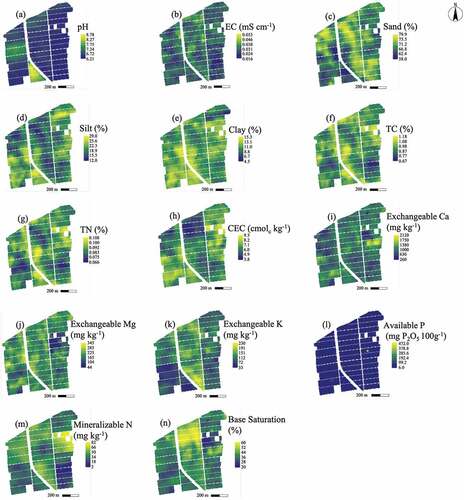
TC, TN, sand, and EC showed strong variability across the fields (Figure 2). On the other hand, pH, mineralizable N, available P, exchangeable K, exchangeable Ca, and exchangeable Mg exhibited less within-field variability. The spatial distribution of TC was similar to that of TN, with contents higher in the central and south-central regions. The spatial distribution of particle size distribution (silt and clay), TC, TN, and CEC also showed a similar pattern. The pH and available P basically did not change so much across the fields and exhibited hotspots with extremely high values in certain areas in a couple of fields. The silt content was lower in areas with high sand content.

Figure 2. Interpolated spatial patterns of soil properties. (a) pH, (b) EC, (c) sand, (d) silt, (e) clay, (f) TC, (g) TN, (h) CEC, (i) exchangeable Ca, (j) exchangeable Mg, (k) exchangeable K, (l) available P, (m) mineralizable N, (n) base saturation.

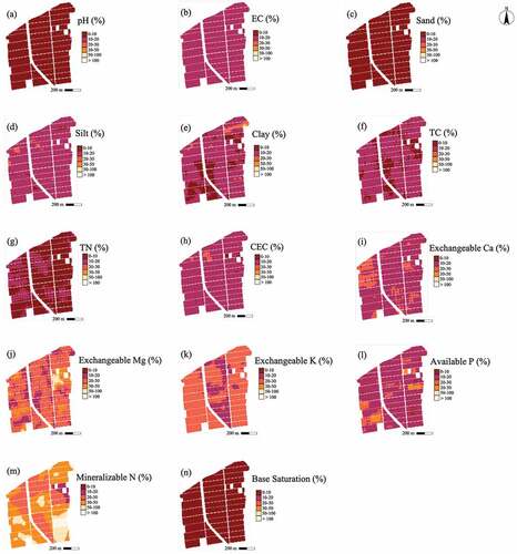
The maps of uncertainty in spatial interpolation are presented as CV distribution maps (Figure 3). The prediction results were highly reliable for pH, sand, and TN, with CV values less than 10% across all fields. Most CV values ranged between 10% and 20% for EC, silt, clay, TC, CEC, exchangeable Ca, and exchangeable Mg, which indicated that the accuracy of those six soil maps was not high. CV values for exchangeable K, available P, and mineralizable N were over 20% in the central areas of the study site.

Figure 3. Coefficients of variation (CV) for soil map prediction. (a) pH, (b) EC, (c) sand, (d) silt, (e) clay, (f) TC, (g) TN, (h) CEC, (i) exchangeable Ca, (j) exchangeable Mg, (k) exchangeable K, (l) available P, and (m) mineralizable N, (n) base saturation.

4. Discussion

4.1. Appropriate sampling size and distance

The present study assessed the effect of sample size on the precision of soil tests to understand field-specific soil properties from the perspective of a design-based approach. In addition, spatial analysis was performed to identify the optimal sampling distances for spatial interpolation and to assess potential applications in soil mapping from the perspective of a model-based approach. The traditional sampling method is usually set at three to five samples per field in Japan. The great concern is whether sample sizes are sufficient to obtain precise results in soil tests with recent land consolidation and enlargement of the scale of farming in Japanese paddy fields. Another question is whether within-field spatial variability should be considered if the traditional sampling method is not reliable.

In common with a previous study (Yanai et al. 2008), the results of the bootstrap method showed that pH and sand percentage can achieve highly reliable characterization even at very low sample sizes (Table 3). The pH values ranged from 6 to 9, and only 3% of pH values were over 8 (Figure 2). Furthermore, there was seemingly little within-field variability in pH, and spatially identical values were present at the block-specific scale rather than the field-specific scale (Figure 2). On the other hand, base saturation was not significantly correlated with pH (Table 2). The result was inconsistent with previous studies reporting that there were strong positive relationships between base saturation and pH (Kabała and Łabaz 2018; Grand and Lavkulich 2013). Furthermore, there was a clear within-field variability of base saturation (Figure 2). These results might be due to the lack of other bases such as sodium in the calculation of base saturation. Indeed, there were no theoretical explanation for no significant relationships between base saturation and pH, but the relatively uniform spatial distribution of pH in a certain block might be due to the paddling paddy fields or flooding that has a stirring effect. Overall, the results indicate that traditional soil sampling can provide sufficient information for liming. Although local farmers have applied lime uniformly in past years, the pH showed extremely high values in the south-central region, which indicates that uniform liming should be avoided for this area. Soil sampling for pH adjustment could be further reduced, which would help decrease the cost of soil collection and analysis. For instance, a couple of soil samples from each block might be sufficient for pH adjustment. Although previous studies have highlighted the importance of VRA for lime application based on soil pH maps (Bönecke et al. 2021; Bogunovic et al. 2014), VRA may not be necessary for large-scale paddy fields considering the farming scale. However, the recommendation can only be applicable to this region, and further investigation is needed to reach more robust conclusions.

The results of bootstrap estimation show that EC, exchangeable Mg, exchangeable K, available P, and mineralizable N cannot meet the precision requirements for field-specific values in most of the fields even at the hypothetical maximum sample size (n = 12). Yanai et al. (2008) also highlighted that exchangeable K, available P, and mineralizable N had a relatively high estimation error at the probability level of 95%. Thus, most of the available nutrients were not able to be characterized with high precision even with the maximum sample size. This might be because the exchangeable cations and available nutrients have been affected by external factors other than parent materials, as previous studies suggested that different management practices such as fertilizer application, irrigation, and tillage could cause large spatial variability in nutrients, organic matter, and pollutants (Akram et al. 2018; Tang et al. 2021). Ideally, it is necessary to increase the number of samples to improve the accuracy of surveys, but it is impractical to collect such a large number of samples.

Note that no precision requirement could be achieved for exchangeable K or mineralizable N. Furthermore, the sill-to-nugget ratios of exchangeable K and mineralizable N were 0.495 and 0.518, respectively (Table 2), suggesting that approximately half of the variation can be explained by random factors. For these two soil properties, increasing the sample size is not effective for improving measurement precision, and we should note that it would be highly variable even at a fine scale. Due to the low measurement precision and intensive sampling costs, it is not practical to collect soil samples at a finer scale if a soil test focuses on the measurement of exchangeable K and mineralizable N. The strong spatial dependency of soil measurements is attributed to inherent characteristics of soils, such as soil parent material, soil texture, topography, and vegetation (Wang et al. 2008; Juhos, Szabó, and Ladányi 2016). It can lead to strong spatial correlation of soil nutrients, while weak spatial dependency of soil properties indicates that spatial variability is mainly regulated by external factors, such as fertilization and cultivation practices (Kılıç, Özgöz, and Akbaş 2004; Wang et al. 2008; Ortega et al. 1999; Fu et al. 2014; Guan et al. 2017).

Therefore, traditional sampling methods might not be sufficiently reliable if farmers want to know the contents of available nutrients in particular fields. Schut and Giller (2020) similarly argued that a field-specific fertilizer recommendation based on a single composite soil sample is a pipe dream because of the large errors of soil tests derived not only from soil sampling but also from chemical analysis procedures. In practical situations, errors due to soil analysis are not negligible. Thus, geostatistical analysis, namely model-based approach, might be a useful tool as it can allow establishment of rational sampling distance, spatial interpolation, and uncertainty estimation, i.e., nugget-to-sill ratios represent a degree of measurement error.

The distance between sampling points should be less than half of the range parameter for spatial interpolation in the geostatistical framework (Kerry and Oliver 2004). The optimal sampling distance for each soil property excluding exchangeable K and mineralizable N whose nugget variance was very high was as follows: pH: 163 m, EC: 15 m, sand: 30 m, silt: 26 m, clay: 33 m, TC: 24 m, TN: 29 m, CEC: 30 m, exchangeable Ca: 21 m, exchangeable Mg: 17 m, and available P: 24 m. The results showed that the recommended sampling distance was shortest for EC (15 m) among all soil properties. Sampling should in principle be conducted at 15-m intervals if all soil properties meet the requirement; however, such a sampling design would consequently increase the number of samples. For instance, approximately 50 soil samples might be needed at the typical field scale (50 m × 200 m) in this region. For EC, the issue of sampling cost can be mitigated by using an on-the-go soil EC sensor. Based on the range parameter values of the other properties, a reasonable sampling interval should be set at approximately 20 m if all soil properties but exchangeable K and mineralizable N are the concerns of soil test. Note that the result of geostatistical analysis was based on the data collected from spatially neighboring 43 fields (0.64 km²). Thus, the recommended sampling distance may vary if practitioners prefer to investigate the within-field heterogeneity of soil properties in a single large-scale paddy field.

4.2. Spatial variability and uncertainty

There were similar and large spatial variations in particle size distribution (silt and clay), TC, TN, and CEC (Figure 2) with the CV values ranging from 0% to 20% (Figure 3). These soil properties were significantly correlated with each other (Table 2). The results highlight the potential need of site-specific management for optimizing fertilizer application rates due to the high spatial variability in soil properties relevant to soil fertility and drainage.

For EC, exchangeable Ca, exchangeable Mg, exchangeable K, available P, and mineralizable N, over 50% of fields did not meet the precision of 10% allowable error even with the maximum sample size (i.e., n = 12) (Table 1). Strong spatial dependencies and relatively short ranges were found for EC, exchangeable Ca, exchangeable Mg, and available P (Table 2). Although an attempt to reduce the cost of sampling is needed, the results indicate that the spatial interpolation method is one of the solutions for facilitating understanding of soil spatial patterns to support robust decision-making for implementing site-specific management. In addition, large nugget-to-sill ratios were found for exchangeable K and mineralizable N (Table 2). The uncertainty maps represented by CV distributions further indicate low prediction performance for these soil properties (Figure 3). For instance, the CV values for mineralizable N exceeded 50% in approximately 17% of the total area. Therefore, it should be borne in mind that these available nutrients, such as exchangeable K and mineralizable N, are highly variable even when the soil maps are generated based on a geostatistical approach. Thus, from a practical viewpoint, conventional design-based sampling design that has been commonly conducted by local agricultural advisory services is the best approach for the highly variable soil properties. Overall, there was great uncertainty in the estimates of soil properties, although the soil samples were collected more densely than in the conventional method. From a practical viewpoint, to improve the accuracy of soil mapping without increasing the cost of soil sampling and analysis, the application of spectral soil analysis or spatial covariates from freely available satellite imagery and climate data should be combined with machine learning approaches (Hengl et al. 2021; Padarian, Minasny, and McBratney 2019; de Santana et al. 2021).

Various anthropogenic activities have weakened spatial correlations of soil properties, such as nutrients and heavy metals, and have caused soils to develop in the direction of spatial homogenization (Wu et al. 2019; Tang et al. 2021). Therefore, the historical impacts of crop management (e.g., crop, fertilization, tillage, and irrigation) on the spatial variability of soil properties should be considered to include such spatial trends. Based on AIC values, LMMs incorporating crop type and/or crop rotation block as fixed effects (Models 1 and 2) were selected for all soil properties excluding pH and sand content. Although we did not apply space-time analysis explicitly, the results indicate that these soil properties have been affected by crop types and rotation. Thus, it might be necessary to measure these soil properties in every season before planting each crop. The degree of temporal changes in soil properties should be assessed in further studies.

5. Conclusions

Soil sampling design is an essential step for precise measurement of soil properties, which helps provide farmers with reliable information about crop management. The present study demonstrated that appropriate soil sampling design and the subsequent soil management practices might differ according to specific soil properties in large-scale paddy fields. To assess precise field-specific values, traditional sampling methods with few replications can be used for pH and sand content only. According to the soil maps, lime application rates can be reduced with little sampling effort for pH measurement. Field-specific uniform application rather than variable-rate application is recommended for liming. Regarding other soil properties, it is recommended to integrate geostatistical analysis into sampling design for better understanding of spatial uncertainty. Soil sampling distances are recommended as 15–163 m, depending on specific soil properties. Geostatistical analysis and the following site-specific management may have a potential for improving crop productivity or for reducing the cost of fertilization as there were large within-field variabilities in several soil properties (e.g., soil particle size distribution and CEC) relevant to soil fertility and drainage. Although the field-specific values of EC, exchangeable Mg, and available P are not precise, these properties can be estimated by the spatial interpolation method, and potential applications in site-specific management should be examined in further studies. On the other hand, it was difficult to obtain reliable estimates of exchangeable K and mineralizable N, because high levels of spatial uncertainty were detected by geostatistical analysis. Therefore, local crop advisories and farmers should note that outcomes from soil tests inherently include fine-scale errors in several available nutrients such as exchangeable K and mineralizable N irrespective of aspects of sampling design including both design-based and model-based approaches. Soil is the final product of complicated interactions among climate, topography, parent materials, and agronomic practices. Further research will be carried out to assess these interactions by using machine learning approaches to provide more robust and reliable soil maps with less sampling effort.

Acknowledgments

The present study was conducted using the ICP-AES of the Division of Instrument Analysis, Gifu University.

Disclosure statement

The authors report there are no competing interests to declare.

Additional information

Funding

This work was supported by a Japan Society for the Promotion of Science (JSPS) KAKENHI Early-Career Scientists Grant (number 18K14452) and a Japan Science and Technology Agency (JST) ACT-X grant (JPMJAX20AF).

References

- Ahuja, L. R. 2003. “Quantifying Agricultural Management Effects on Soil Properties and Processes.” Geoderma 116 (1–2): 1–2. doi:10.1016/S0016-7061(03)00090-9.
- Akaike, H. 1998. “Information Theory and an Extension of the Maximum Likelihood Principle.” In Selected Papers of Hirotugu Akaike, edited by Parzen, E., Tanabe, K., Kitagawa, G., 199–213. New York, NY: Springer.
- Akram, R., V. Turan, H. M. Hammad, S. Ahmad, S. Hussain, A. Hasnain, and M. M. Maqbool, et al. 2018. “Fate of Organic and Inorganic Pollutants in Paddy Soils .” In Environmental Pollution of Paddy Soils, edited by Hashmi, M.Z. and Varma, A. 197–214. Cham: Springer.
- Bhakta, I., S. Phadikar, and K. Majumder. 2019. “State‐of‐the‐art Technologies in Precision Agriculture: A Systematic Review.” Journal of the Science of Food and Agriculture 99 (11): 4878–4888. doi:10.1002/jsfa.9693.
- Bogunovic, I., M. Mesic, Z. Zgorelec, A. Jurisic, and D. Bilandzija. 2014. “Spatial Variation of Soil Nutrients on sandy-loam Soil.” Soil and Tillage Research 144: 174–183. doi:10.1016/j.still.2014.07.020.
- Bönecke, E., S. Meyer, S. Vogel, I. Schröter, R. Gebbers, C. Kling, E. Kramer, et al. 2021. “Guidelines for Precise Lime Management Based on high-resolution Soil pH, Texture and SOM Maps Generated from Proximal Soil Sensing Data.” Precision Agriculture 22 (2): 493–523. doi:10.1007/s11119-020-09766-8.
- Box, G. E. P., and D. R. Cox. 1964. “An Analysis of Transformations.” Journal of the Royal Statistical Society: Series B (Methodological) 26 (2): 211–243. doi:10.1111/j.2517-6161.1964.tb00553.x.
- Brus, D. J., and J. J. De Gruijter. 1997. “Random Sampling or Geostatistical Modelling? Choosing between design-based and model-based Sampling Strategies for Soil (With Discussion).” Geoderma 80 (1–2): 1–44. doi:10.1016/S0016-7061(97)00072-4.
- Brus, D. J. 2021. “Statistical Approaches for Spatial Sample Survey: Persistent Misconceptions and New Developments.” European Journal of Soil Science 72 (2): 686–703. doi:10.1111/ejss.12988.
- Cambardella, C. A., T. B. Moorman, J. M. Novak, T. B. Parkin, D. L. Karlen, R. F. Turco, and A. E. Konopka. 1994. “Field‐scale Variability of Soil Properties in Central Iowa Soils.” Soil Science Society of America Journal 58 (5): 1501–1511. doi:10.2136/sssaj1994.03615995005800050033x.
- Carré, F., A. B. McBratney, T. Mayr, and L. Montanarella. 2007. “Digital Soil Assessments: Beyond DSM.” Geoderma 142 (1–2): 69–79. doi:10.1016/j.geoderma.2007.08.015.
- Carter, M. R., and E. G. Gregorich. 2007. Soil Sampling and Methods of Analysis. Boca Raton: CRC press. Boca Raton.
- Cataldo, D. A., M. Maroon, L. E. Schrader, and V. L. Youngs. 1975. “Rapid Colorimetric Determination of Nitrate in Plant Tissue by Nitration of Salicylic Acid.” Communications in Soil Science and Plant Analysis 6 (1): 71–80. doi:10.1080/00103627509366547.
- Curran, P. J. 1988. “The Semivariogram in Remote Sensing: An Introduction.” Remote Sensing of Environment 24 (3): 493–507. doi:10.1016/0034-4257(88)90021-1.
- De Gruijter, J. J., and C. J. F. Ter Braak. 1990. “Model-free Estimation from Spatial Samples: A Reappraisal of Classical Sampling Theory.” Mathematical Geology 22 (4): 407–415. doi:10.1007/BF00890327.
- de Santana, F. B., S. K. Otani, A. M. de Souza, and R. J. Poppi. 2021. “Comparison of PLS and SVM Models for Soil Organic Matter and Particle Size Using vis-NIR Spectral Libraries.” Geoderma Regional 27: e00436. doi:10.1016/j.geodrs.2021.e00436.
- Efron, B. 1979. “Bootstrap Methods: Another Look at the Jackknife.” The Annals of Statistics 7 (1:) 1–26.
- Fu, W., P. Jiang, K. Zhao, G. Zhou, Y. Li, J. Wu, and H. Du. 2014. “The Carbon Storage in Moso Bamboo Plantation and Its Spatial Variation in Anji County of Southeastern China.” Journal of Soils and Sediments 14 (2): 320–329. doi:10.1007/s11368-013-0665-7.
- Gee, G. W., and J. W. Bauder 1986. ”Particle Size Analysis Klute, A.” In Methods of Soil Analysis: Part IMethods of Soil Analysis: Part I, 2ndVol. 9pp. 383–411. Wisconsin, USA: SSSA and ASA.
- Goovaerts, P. 1999. ““Geostatistics in Soil Science: State-of-the-art and Perspectives.” Geoderma 89 (1–2): 1–45. doi:10.1016/S0016-7061(98)00078-0.
- Grand, S., and L. M. Lavkulich. 2013. “Potential Influence of Poorly Crystalline Minerals on Soil Chemistry in Podzols of Southwestern Canada.” European Journal of Soil Science 64 (5): 651–660. doi:10.1111/ejss.12062.
- Guan, F., M. Xia, X. Tang, and S. Fan. 2017. “Spatial Variability of Soil Nitrogen, Phosphorus and Potassium Contents in Moso Bamboo Forests in Yong’an City, China.” Catena 150: 161–172. doi:10.1016/j.catena.2016.11.017.
- Hengl, T., M. A. Miller, J. Križan, K. D. Shepherd, A. Sila, M. Kilibarda, J. Crouch, et al. 2021. “African Soil Properties and Nutrients Mapped at 30 M Spatial Resolution Using two-scale Ensemble Machine Learning.” Scientific Reports 11 (1): 1–18. doi:10.1038/s41598-021-85639-y.
- Hesterberg, T. 2011. “Bootstrap.” Wiley Interdisciplinary Reviews: Computational Statistics 3 (6): 497–526. doi:10.1002/wics.182.
- Inoko, A. 1986. Available N Onikura, Y Standard Methods of Soil Analysis and Measurement, (Tokyo, Japan: Hakuyuusha), 118–121.
- Jianwei, L. 2019. “Sampling Soils in a Heterogeneous Research Plot.” JoVE (Journal of Visualized Experiments) 143: e58519. doi:10.3791/58519.
- Juhos, K., S. Szabó, and M. Ladányi. 2016. “Explore the Influence of Soil Quality on Crop Yield Using statistically-derived Pedological Indicators.” Ecological Indicators 63: 366–373. doi:10.1016/j.ecolind.2015.12.029.
- Kabała, C., and B. Łabaz. 2018. “Relationships between Soil pH and Base Saturation - Conclusions for Polish and internationaGranl Soil Classifications.” Soil Science Annual 69 (4): 206–214. doi:10.2478/ssa-2018-0021.
- Keeney, D. R., and D. W. Nelson. 1983. “Nitrogen—inorganic Forms.” Methods of Soil Analysis: Part 2 Chemical and Microbiological Properties, 643–698.
- Kerry, R., and M. A. Oliver. 2004. “Average Variograms to Guide Soil Sampling.” International Journal of Applied Earth Observation and Geoinformation 5 (4): 307–325. doi:10.1016/j.jag.2004.07.005.
- Kılıç, K., E. Özgöz, and F. Akbaş. 2004. “Assessment of Spatial Variability in Penetration Resistance as Related to Some Soil Physical Properties of Two Fluvents in Turkey.” Soil and Tillage Research 76 (1): 1–11. doi:10.1016/j.still.2003.08.009.
- Li, J., D. Richter, A. Mendoza, and P. Heine. 2010. “Effects of land-use History on Soil Spatial Heterogeneity of Macro- and Trace Elements in the Southern Piedmont USA.” Geoderma 156 (1–2): 60–73. doi:10.1016/j.geoderma.2010.01.008.
- López-Granados, F., M. Jurado-Expósito, J. M. Peña-Barragán, and L. García-Torres. 2005. “Using Geostatistical and Remote Sensing Approaches for Mapping Soil Properties.” European Journal of Agronomy 23 (3): 279–289. doi:10.1016/j.eja.2004.12.003.
- Moritsuka, N., J. Yanai, M. Umeda, and D. Kosaki. 2004. “Spatial Relationships among Different Forms of Soil Nutrients in a Paddy Field.” Soil Science and Plant Nutrition 50 (4): 565–573. doi:10.1080/00380768.2004.10408513.
- Mzuku, M., R. Khosla, R. Reich, D. Inman, F. Smith, and L. MacDonald. 2005. “Spatial Variability of Measured Soil Properties across Site-Specific Management Zones.” Soil Science Society of America Journal 69 (5): 1572–1579. doi:10.2136/sssaj2005.0062.
- Ortega, R. A., D. G. Westfall, W. J. Gangloff, and G. A. Peterson 1999. “Multivariate Approach to N and P Recommendations in Variable Rate Fertilizer Applications. In Precision Agriculture’99, Part 1 and Part 2.” Papers presented at the 2nd European Conference on Precision Agriculture, Odense, Denmark. Sheffield Academic Press.
- Padarian, J., B. Minasny, and A. B. McBratney. 2019. “Using Deep Learning to Predict Soil Properties from Regional Spectral Data.” Geoderma Regional 16: e00198. doi:10.1016/j.geodrs.2018.e00198.
- Pii, Y., S. Cesco, and T. Mimmo. 2015. “Shoot Ionome to Predict the Synergism and Antagonism between Nutrients as Affected by Substrate and Physiological Status.” Plant Physiology and Biochemistry 94: 48–56. doi:10.1016/j.plaphy.2015.05.002.
- Ribeiro, P. J., and P. J. Diggle. 2001. “The geoR Package.” R-NEWS 1: 15–18.
- Sato, H. 2001. “The Current State of Paddy Agriculture in Japan 1.” Irrigation and Drainage: The Journal of the International Commission on Irrigation and Drainage 50 (2): 91–99. doi:10.1002/ird.10.
- Schut, A. G. T., and K. E. Giller. 2020. “Soil-based, field-specific Fertilizer Recommendations are a pipe-dream.” Geoderma 380: 114680. doi:10.1016/j.geoderma.2020.114680.
- Shao, J. 1996. “Bootstrap Model Selection.” Journal of the American Statistical Association 91 (434): 655–665. doi:10.1080/01621459.1996.10476934.
- Stefano, C. D., V. Ferro, and P. Porto. 2000. “Applying the Bootstrap Technique for Studying Soil Redistribution by Caesium-137 Measurements at Basin Scale.” Hydrological Sciences Journal 45 (2): 171–183. doi:10.1080/02626660009492318.
- Tan, K. 2005. Soil Sampling, Preparation, and Analysis CRC Press. Boca Raton, FL: Marcel Dekker.
- Tanaka, T. S. T., Y. Kono, and T. Matsui. 2019. “Assessing the Spatial Variability of Winter Wheat Yield in large-scale Paddy Fields of Japan Using Structural Equation Modelling. Precis Precision Agriculture’19. 19. Wageningen Academic Publishers. doi:10.3920/978-90-8686-888-9_93.
- Tang, X., Y. Wu, Z. Lan, L. Han, and X. Rong. 2021. “Analysis of the Spatial Distribution of Heavy Metals in an Area of Farmland in Sichuan Province, China.” Environmental Earth Sciences 80 (8): 1–11. doi:10.1007/s12665-021-09612-8.
- Tomasi, N., T. Mimmo, R. Terzano, M. Alfeld, K. Janssens, L. Zanin, S. Cesco, Z. Varanini, and R. Pinton. 2014. “Nutrient Accumulation in Leaves of Fe-deficient Cucumber Plants Treated with Natural Fe Complexes.” Biology and Fertility of Soils 50 (6): 973–982. doi:10.1007/s00374-014-0919-6.
- Truog, E. 1930. “The Determination of the Readily Available Phosphorus of Soils 1.” Journal of the American Society of Agronomy 22 (10): 874–882. doi:10.2134/agronj1930.00021962002200100008x.
- Wang, G., J. Innes, S. Dai, and G. He. 2008. “Achieving Sustainable Rural Development in Southern China: The Contribution of Bamboo Forestry.” The International Journal of Sustainable Development & World Ecology 15 (5): 484–495. doi:10.3843/SusDev.15.5:9.
- Webster, R., and M. A. Oliver. 1992. “Sample Adequately to Estimate Variograms of Soil Properties.” Journal of Soil Science 43 (1): 177–192. doi:10.1111/j.1365-2389.1992.tb00128.x.
- Webster, R., and M. A. Oliver. 2007. Geostatistics for Environmental Scientists. England: John Wiley & Sons.
- Wu, C., J. Huang, H. Zhu, L. Zhang, B. Minasny, B. P. Marchant, and A. B. McBratney. 2019. “Spatial Changes in Soil Chemical Properties in an Agricultural Zone in Southeastern China Due to Land Consolidation.” Soil and Tillage Research 187: 152–160. doi:10.1016/j.still.2018.12.012.
- Yanai, J., C. K. Lee, M. Umeda, and T. Kosaki. 2000. “Spatial Variability of Soil Chemical Properties in a Paddy Field.” Soil Science and Plant Nutrition 46 (2): 473–482. doi:10.1080/00380768.2000.10408800.
- Yanai, J., C. K. Lee, T. Kaho, M. Iida, T. Matsui, M. Umeda, and T. Kosaki. 2001. “Geostatistical Analysis of Soil Chemical Properties and Rice Yield in a Paddy Field and Application to the Analysis of yield-determining Factors.” Soil Science and Plant Nutrition 47 (2): 291–301. doi:10.1080/00380768.2001.10408393.
- Yanai, J., T. Matsubara, C. K. Lee, N. Moritsuka, H. Shinjo, and T. Kosaki. 2008. “Establishment of Rational Soil Sampling Scheme for the Paddy Field – Relationship between Sampling Frequency and Data Reliability.” Japanese Journal of Soil Science and Plant Nutrition 79 61–67. in Japanese with English summary
- Zhou, X., G. B. M. Heuvelink, Y. Kono, T. Matsui, and T. S. T. Tanaka. 2022. “Using Linear mixed-effects Modeling to Evaluate the Impact of Edaphic Factors on Spatial Variation in Winter Wheat Grain Yield in Japanese Consolidated Paddy Fields.” European Journal of Agronomy 133: 126447. doi:10.1016/j.eja.2021.126447.
- Zimmerman, D., and M. Zimmerman. 1991. “A Comparison of Spatial Semivariogram Estimators and Corresponding Ordinary Kriging Predictors.” Technometrics 33 (1): 77–91. doi:10.1080/00401706.1991.10484771.
- Zoubir, A. M., and D. R. Iskandler. 2007. “Bootstrap Methods and Applications.” IEEE Signal Processing Magazine 24 (4): 10–19. doi:10.1109/MSP.2007.4286560.