Research and Development of a Photogrammetric Condition Monitoring Workflow to Improve Change Detection in Wall Paintings

ABSTRACT

In the field of wall painting conservation, condition monitoring plays a key role in assessing the stability of a painting by determining if detrimental change is occurring over time. Condition monitoring typically involves a visual comparison between the painting and a previously captured photograph or image and relies on the ability of a conservator to observe visible change. In practice, the monitoring of wall paintings can be challenging given the potential range of condition phenomena, complexity of material composition, uneven surface topography and issues of scale, access, and lighting. Using two-dimensional images alone to detect change, across large surface areas and in depth, is often insufficient and can result in misleading or incomplete assessments of condition. To improve the detection of change in wall paintings, the Getty Conservation Institute initiated research between conservators and heritage recording specialists to update and validate a photogrammetric condition monitoring workflow that can identify three-dimensional change using readily available and cost-effective equipment. This paper describes the workflow and the experimental trials conducted to characterize its precision and accuracy. The results of this initial research demonstrate that an affordable, photogrammetric workflow can reliably detect and quantify sub-millimeter change in wall paintings, improving current condition monitoring practice.

KEYWORDS:

• Condition monitoring
• wall paintings
• photogrammetry
• change detection
• imaging

Introduction

Condition monitoring, defined as the systematic collection of comparable condition data to measure change, is a key component of an overall conservation strategy, helping to assess the stability of a painting (Wong et al. 2021a). It involves the visual comparison of previously captured images against the current condition of a wall painting. The scope of the condition monitoring can vary and should be based on the defined conservation needs of the wall painting and its context. For example, condition monitoring can be used as a diagnostic tool to detect detrimental change in a wall painting, to identify causes of deterioration, and to evaluate vulnerability and risk.

Wall paintings are often thought of as two-dimensional surfaces, but in reality they are three-dimensional in nature, exhibiting complex condition phenomena such as paint flaking, plaster deformation, and cracking, both at the surface and in depth. Identifying three-dimensional changes across a large painting using two-dimensional images alone is often insufficient and can result in a misleading or incomplete assessment of condition. This challenge is exacerbated by wall paintings’ complexity of material composition, uneven surface topography, and issues of scale, access, and lighting.

To improve the assessment of condition in wall paintings, the Getty Conservation Institute initiated research between conservators and heritage recording specialists to update and validate a photogrammetric condition monitoring workflow that has been shown to identify three-dimensional change using readily available and cost-effective equipment. This paper describes the workflow and the experimental lab-based trials conducted to characterize its precision and accuracy. The results of this initial research demonstrate that an affordable photogrammetric workflow can improve current condition monitoring practice by reliably detecting and quantifying sub-millimeter three-dimensional change in wall paintings.

Photogrammetric condition monitoring workflow

Structure from Motion (SfM) photogrammetry is an increasingly used technique to document wall paintings that generates scaled three-dimensional models from overlapping two-dimensional images taken with a standard camera (Lucet 2013; Percy et al. 2015; Reina Ortiz et al. 2019; Wong et al. 2021b) Photogrammetric software identifies common groups of pixels in an image block (a set of images taken to generate a photogrammetric model) and calculates their relative three-dimensional location using image metadata containing information about the camera, lens, and focal length.

Photogrammetry has significant advantages for monitoring wall paintings over other three-dimensional documentation techniques, such as laser scanning, as the equipment required is minimal (a camera and light source) and cost-effective (Abate et al. 2014). Photogrammetry also provides greater flexibility by enabling capture of a subject at a range of spatial resolutions,¹ as this can be adjusted by altering the camera, lens, focal length, and/or distance between the camera and the subject.

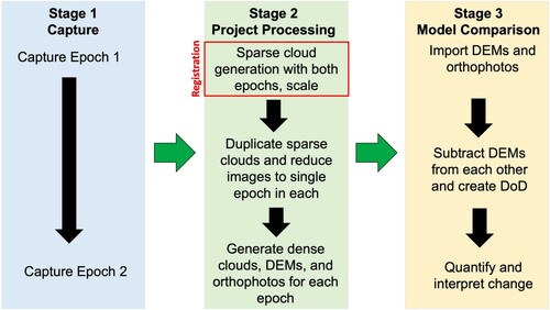
Photogrammetric monitoring compares three-dimensional models of a subject from different points in time to detect and quantify volumetric change. A photogrammetric monitoring workflow was tested to determine the limits of precision and accuracy of change detection. This workflow consists of three stages: capture, project processing, and model comparison (Figure 1).

Figure 1. In the tested photogrammetric monitoring workflow digital elevation models (DEM) are generated from two image blocks (referred to as epochs as they are part of a monitoring program) and are compared to create the DEM of difference (DoD) to identify and quantify change. © J. Paul Getty Trust

Stage 1: capture

During the capture stage, a pre-determined monitoring area is captured in an image block repeatedly over time. Each image block that is captured as part of a photogrammetric monitoring program is referred to as an epoch as it records the wall painting at a single point in time. To reduce variability and to enable reproducibility, a protocol was established to ensure consistency of capture for each epoch. The capture protocol specifies the photographic equipment and its settings, the distance of the camera to the subject, the percentage of image overlap, the camera position during capture (i.e. the capture geometry), and the light source and its location in relation to the subject.

Camera geometry

Photogrammetric software requires a minimum of 60% overlap in the images captured with the camera sensor parallel to the subject to generate a three-dimensional model. Incorporating additional images, taken with the camera tilted relative to the subject, referred to as convergent imagery, improves the three-dimensional geometry of the model (García-León, Felicísimo, and Martínez 2003; Wackrow and Chandler 2008; Nocerino, Menna, and Remondino 2014). In the tested workflow, the subject was captured with 66% overlap (due to the ease of visualizing two-thirds overlap), first with the camera parallel to the surface, then tilted upwards, and finally with the camera tilted downwards. The degree of tilt was defined by the depth of field of the camera setup.²

Lighting

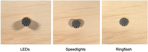
Achieving even lighting can be a significant challenge in the photogrammetric survey of wall paintings due to their large scale and complex environments (Wong et al. 2021b). Wall paintings are often artificially lit during photogrammetric surveys with LED panels or flashes. Even and consistent lighting across epochs is critical for monitoring as different patterns of light and shadow can suggest changes that do not exist. This research looked at the effect of different light sources (LED panels, flashes, and a ring flash) on the precision and accuracy of the detected change.

Stage 2: project processing

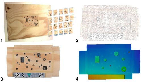
In the project processing stage, three-dimensional models are generated from the image block with photogrammetric software (Figure 2). The image blocks are imported into a project in Agisoft Metashape Professional (v.1.7.2) and pixel groups with high contrast or unique patterns are identified by the software (Agisoft LLC 2021). These pixel groups are then matched by the software across a minimum of two images, providing a set of corresponding points for the overlapping images, known as tie points. The three-dimensional locations of the tie points are calculated by the software and a sparse cloud of points is created as a rough structure of the model. Based on the sparse cloud structure, the three-dimensional model is filled in with the remaining pixel groups, creating a dense point cloud. The dense cloud is then processed into a digital elevation model (DEM) which is an image file where each pixel represents a height value. The DEM is visualized as a heatmap, so an orthophoto, or rectified image, of each epoch is generated to aid in the interpretation of detected change.

Figure 2. The steps taken to generate a three-dimensional model. Step 1: Overlapping images are captured and then imported into the photogrammetric software. Step 2: The images are processed to create a sparse cloud. Step 3: A dense cloud is generated based on the sparse cloud. Step 4: The dense cloud can then be processed into a digital elevation model (DEM) where the relative heights are represented as a heatmap. © J. Paul Getty Trust

Registration

To compare two three-dimensional models digitally and identify differences between them, the models of each epoch need to be precisely registered. Registration is typically achieved by creating or finding the same points in the two epochs and aligning them in the model comparison stage. A registration technique proposed by Feurer and Vinatier (2018) for archival aerial imagery was adapted and applied to change detection in wall paintings by Rose et al. (2021). In this method, multiple epochs are first processed together into a sparse cloud and then scaled. Next, the images are separated into sparse clouds by epoch, and a dense cloud, DEM, and an orthophoto are generated for each. The registration process assumes that a significant number of common features will exist between epochs, allowing the images themselves to provide the reference system without relying on physical targets, which are not always safe to use on fragile painted surfaces.

Stage 3: model comparison

In the model comparison stage, the DEM and orthophoto of each epoch are imported into QGIS (v.3.10.14 – A Coruña), a free and open-source geographic information system (QGIS 2021). The DEMs are subtracted to create a DEM of difference (DoD), a DEM where each pixel represents the difference between epochs. The DoD can be visualized as a heatmap and the change at any point, area, or volume is calculated in the software. When imported, the orthophoto is automatically layered on the DEM and can be used to investigate the relationship between the volumetric change detected and the specific condition of the wall painting.

Experimental trials

Experimental trials were designed to evaluate the accuracy and precision of the overall workflow, and to test the effect of lighting on the results. In these trials, accuracy is used to indicate the difference between the change detected and the actual measurable change that has occurred. Precision refers to the repeatability of the method (i.e. the capacity of the method to detect the same change using an identical setup). Precision is often expressed as the standard deviation σ (sigma), which represents the variability and noise in the measurements written as a ± range. Changes detected that are larger than three standard deviations or 3σ are sufficiently large to be distinguishable from noise, so this is considered the detection limit of the workflow.

Test board set-up

A 40 cm × 20 cm monitoring area was demarcated at the center of a 121 cm × 60 cm plywood board fixed to a wall. The monitoring area allowed each epoch to be captured in sixty photographs. The number of images was determined by the necessary camera geometry and field of view when placed at the camera’s closest possible focus distance to achieve maximum spatial resolution.

During the trials, objects were added and removed from the board between epochs to simulate change events. Sixteen patterned square labels numbered 1 through 16 were applied to the monitoring area. The patterned adhesive labels provided an easily removeable feature and served as both measurable reference points and unique features. At a later stage eight assorted objects of known thicknesses were also applied (Figure 3). A calibrated scale bar with photogrammetric targets was placed below the monitoring area.³ The centers of the coded targets on the scale bar were identified in the project processing stage to scale the model to 0.01 mm precision.⁴

Figure 3. Patterned adhesive labels were affixed to the monitoring area to create distinct features for photogrammetric model generation (top). Objects numbered 1–8 (with the prefix H) were added to the board (bottom) and their height on the board was determined by taking and averaging measurements using a vernier caliper on four points of each object. © J. Paul Getty Trust

Equipment

A Sony α7R II with back-illuminated full-frame image sensor camera and Sony Sonnar T* FE 55 mm f/1.8 ZA lens were used for the trials. Three different light sources were tested including two Neewer 660 LED panels (40W, 3360 lumens) angled 45° towards the test board, two Sony HVL-F60RM flashes (handheld and on an armature) angled 45° towards the test board, and a Nissin MF18 Macro ring flash attached to the end of the lens. A Manfrotto 475B Pro Geared Tripod with a Sirui FD-01 Four-Way Head was used when capturing the board while it was illuminated by LED panels. Thickness measurements of the labels and added objects were made with a Mitutoyo 530-316 Vernier caliper with a precision of ±0.05 mm.

Experimental set-up

For each trial, the camera was positioned 50 cm away from the test board (Figure 4), resulting in a spatial resolution of 0.03 mm/pixel. The camera and lens were set to ISO 100 and f/8 aperture to minimize noise and diffraction⁵ and optimize the depth of field. Each epoch was captured with the camera parallel with 66% overlap, then with the camera tilted up and down ±5° with 66% overlap. The close distance of the camera to the test board created a narrow depth of field, which limited the camera tilt to ±5° to avoid partially out-of-focus images.

Figure 4. The LED capture set-up with the Sony α7R II on a tripod and two LED panels angled 45° towards the board. External light was blocked out to ensure controlled lighting conditions. © J. Paul Getty Trust

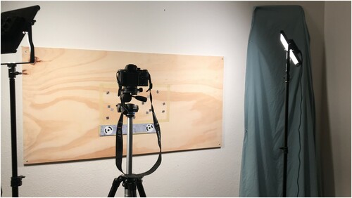
Capture was performed at night to ensure that no external light affected the trials.

Data processing

All captured images were color corrected and processed into uncompressed TIFFs for the project processing stage using Adobe Lightroom Classic (v 10.3). The sparse and dense clouds were processed using Agisoft Metashape on the ‘high’ setting.⁶

Overview of trials

A series of eight experimental trials was designed and undertaken to test specific aspects of the photogrammetric monitoring workflow (Table 1).

Table 1. Trials undertaken to determine the accuracy and precision of the workflow.

Trial		Epoch	Test board set-up	Light source
1	Control – Effect of registration technique	Epoch 1	Sixteen labels	LED panels
		Epoch 2	Sixteen labels	LED panels
2	Change detection – Effect of adding eight measured objects	Epoch 2	Sixteen labels	LED panels
		Epoch 3	Sixteen labels and eight objects	LED panels
3	Change detection – Effect of removing two measured labels	Epoch 3	Sixteen labels and eight objects	LED panels
		Epoch 4	Fourteen labels and eight objects	LED panels
4	Lighting test – Effect of moved LED panels	Epoch 4	Fourteen labels and eight objects	LED panels
		Epoch 5	Fourteen labels and eight objects	LEDs 20° towards the board
5	Lighting test – Effect of handheld flashes	Epoch 6	Fourteen labels and eight objects	Handheld flashes
		Epoch 7	Fourteen labels and eight objects	Handheld flashes
6	Lighting test – Effect of flashes on armature	Epoch 8	Fourteen labels and eight objects	Flashes on armature
		Epoch 9	Fourteen labels and eight objects	Flashes on armature
7	Lighting test – Effect of ring flash	Epoch 10	Fourteen labels and eight objects	Ring flash
		Epoch 11	Fourteen labels and eight objects	Ring flash
8	Lighting test – Effect of two different light sources	Epoch 7	Fourteen labels and eight objects	Handheld flashes
		Epoch 11	Fourteen labels and eight objects	Ring flash

Control trial (Trial 1)

In Trial 1, the monitoring area was captured unchanged in Epochs 1 and 2 with constant lighting to create a control dataset. Epoch 2 was captured immediately after Epoch 1 to ensure that no change occurred to the board. Any difference identified in this trial would represent a discrepancy from the actual lack of change to the test board. Differences within the calculated error level (less than 3σ) could be attributed to noise in the models, whereas differences greater than 3σ would indicate that the workflow inaccurately detected change.

Change detection trials (Trials 2–3)

Trials 2 and 3, comparing Epochs 2 and 3 and Epochs 3 and 4 respectively, tested the workflow’s ability to detect change. In Trial 2, an assortment of eight objects, consisting of coins, washers, and cork stoppers of various sizes and thicknesses were adhered to the board. The objects were covered with patterned labels to provide distinct features to aid in the generation of the point clouds and to block their reflective surfaces, which are difficult to process into three-dimensional models.⁷ The height of each object on the board was measured at four points with the caliper and the mean calculated. The caliper measurements were used as the actual height differences against which to compare the change data on the DoD. Similarly, in Epoch 4, two labels each with a thickness of 0.1 mm were removed from the board to test the ability of the workflow to accurately detect sub-millimeter changes.

Lighting trials (Trials 4–8)

Trials 4–8 tested the effect of light on the precision and accuracy of the workflow by capturing the unchanged monitoring area with different light sources. Each lighting trial tested the same light source captured in two epochs with the board unchanged to determine if the use of that light source and the variations during capture (changing distance and/or orientation relative to the board) resulted in lower precision or accuracy. As Trial 1 demonstrated the precision derived from unmoved LED panels, Trial 4 tested the effect of placing the LED panels at different positions between epochs (45° towards the board compared to 20° towards the board), as can occur when the identical placement of the light source is not possible. In Trial 8, handheld flashes (for Epoch 7) and a ring flash (for Epoch 10) were compared to determine the effect of changing light sources on the workflow results.

Results and discussion

Precision

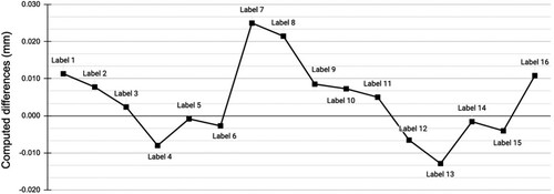
In the control trial comparing Epoch 1 and Epoch 2, measurements were taken on each of the patterned labels on the DoD. As the monitoring area, capture setup, and lighting were unchanged in this trial, the precision of the registration technique could be assessed. The mean difference detected on the sixteen labels was 0.004 mm with a standard deviation of ±0.010 mm (1σ) (Figure 5). As the spatial resolution was 0.03 mm/pixel, the 1-sigma precision of ±0.010 mm indicates that the registration technique closely aligned the two epochs within a single pixel.

Figure 5. The results of the control (Trial 1) comparing Epoch 1 and Epoch 2 show the change detected at each label point and its variation from zero. The small deviation from zero in the dataset shows that the epochs were closely aligned. © J. Paul Getty Trust

Precision: lighting trials

In Trials 4–7, twenty-two points were measured on each DoD (comparing the two epochs with the same light source) and the mean detected change and standard deviation were calculated (Table 2).

Table 2. Mean detected change and standard deviation on the DoD from the control and lighting trials.

Trial	Mean detected change	Standard deviation (σ)
Trial 1 – Control – LED panels	0.004 mm	±0.010 mm
Trial 4 – LED panels replaced 20° towards the board	0.004 mm	±0.019 mm
Trial 5 – Handheld flashes	0.003 mm	±0.015 mm
Trial 6 – Flashes on armature	0.007 mm	±0.014 mm
Trial 7 – Ring flash	−0.006 mm	±0.014 mm
Trial 8 – Ring flash vs handheld flashes	−0.002 mm	±0.031 mm

When the same light source was used consistently over two compared epochs (Trials 4–7), there was no meaningful difference between one light source over another in the precision or accuracy of the results. This was unexpected given the variability in the positioning of the flashes during handheld capture.

In Trial 8, different light sources were compared (capture with handheld flashes compared to capture with a ring flash), which resulted in a σ of ±0.031 mm, double the standard deviation of the trials with the same light source. Similarly, the LED panels that were repositioned at a 20° angle to the board resulted in a slightly higher standard deviation compared to the LEDs placed at the same 45° angle to the board (±0.019 mm compared to ±0.010 mm). This indicates that the light source can influence the precision of the measurements and that the same light source should be used for every capture during the monitoring program to optimize change detection. The light sources also affected the appearance of the generated orthophotos producing different degrees of shadow. The ring flash was notably the only light source that did not cause visible shadows (Figure 6).

Figure 6. The orthophotos generated from the light sources created different shadow patterns on the test board. Only the ring flash resulted in no visible shadows on the orthophoto. © J. Paul Getty Trust

The small mean detected changes indicate the absence of systematic errors in the capture, project processing, and model comparison stages. The standard deviations of changes detected in the lighting trials with the same light source used in the same way were ±0.015 and ±0.014 mm. Two standard deviations are equivalent to the spatial resolution (0.030 mm). Since three standard deviations of the control and lighting trials amount to ±0.045 mm, changes smaller than this can be disregarded as noise. Therefore, with the tested equipment and capture protocol in lab conditions, the workflow could reliably detect changes larger than 0.045 mm.

Accuracy

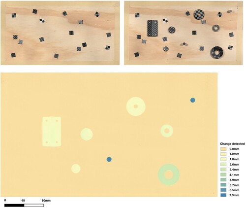
In Trial 2, objects were added to the monitoring area to create detectable change. The DoD heatmap clearly visualized the added objects (Figure 7). The same four points measured on each of the objects with the caliper were measured on the DoD and averaged. The mean difference between the caliper measurements and the digital measurements was 0.05 mm ± 0.128 mm. This trial resulted in lower precision compared to the control and lighting trials. However, the precision of the caliper was ±0.05 mm and the measurements taken on the board were subject to human error. The caliper created an insufficiently accurate reference dataset to give high confidence in change values below 0.1 mm, which limited the ability to assess the accuracy of the workflow in this trial.

Figure 7. In Trial 2, the DEM of difference (DoD) (bottom) reflecting the detected change between Epoch 2 (top left) and Epoch 3 (top right) is shown as a heatmap. © J. Paul Getty Trust

In Trial 3, the adhesive labels with 0.1 mm thickness were removed from the board. This change was detected in the DoD, and measurements showed a mean change of −0.15 mm ± 0.023 mm. This result demonstrates that the workflow was able to detect sub-millimeter change within a tenth of a millimeter accuracy. The change detection in Trial 3 was more accurate than Trial 2, as the labels could be measured prior to their application to the board, reducing human error. However, the precision of the caliper (±0.05 mm) again limited the ability to assess the accuracy of the measurements to hundredths of a millimeter.

Based on the control and lighting trial results when no change was made to the board, the photogrammetric monitoring workflow provided a more accurate measurement of change than the caliper. In future trials, a higher accuracy reference system could be devised to better determine the accuracy of the workflow, although creating a reference with a precision of 0.01 mm or finer is challenging (Remondino et al. 2014).

Conclusions

The photogrammetric monitoring workflow was able to detect and quantify change to a precision of ±0.045 mm at 3σ with the tested equipment, capture protocol, and consistently used light sources in a lab setting. This indicates that in a controlled setting the workflow can detect change larger than 0.045 mm. The results also indicate that all the tested light sources are suitable for a photogrammetric monitoring program if they are used consistently across all epochs. However, the different light sources do produce varying intensities of shadow on the orthophoto, which can affect the interpretation of the results.

Based on these initial lab trials, the workflow shows significant promise in improving methods and approaches to condition monitoring in wall painting conservation by providing consistent quantifiable and objective volumetric change detection. The outcomes also demonstrate the value of collaboration between conservators and heritage recording specialists. The workflow enables the detection and analysis of sub-millimeter three-dimensional changes in wall paintings and provides visual and quantitative data to support conservation decision-making. The next phase of research will apply the condition monitoring workflow to a wall painting site with specific monitoring needs to further refine the method and determine its benefits in real-world conditions.

Acknowledgements

The authors would like to thank and acknowledge the support of colleagues at the Getty Conservation Institute including Susan Macdonald, Head of Building and Sites, and Anna Flavin, Lead Photographer, whose knowledge and assistance in preparing photographic equipment for the experimental trials was indispensable. This research emerged from discussion with colleagues including Mario Santana Quintero at Carleton University and Giulia Russo, GCI Graduate Intern (2018–2019), as well as the many wall painting conservators who have communicated their struggles with condition monitoring. This research was undertaken during the uncertainties of the Covid-19 pandemic which forced us to work remotely and to convert our homes into makeshift laboratories and offices. We gratefully acknowledge our colleagues in the Department of Architecture, Built Environment and Construction Engineering of the Politecnico di Milano, and finally our families who urged us on and patiently endured.

Disclosure statement

No potential conflict of interest was reported by the author(s).

Notes

1 Spatial resolution describes the distance between the centers of two adjacent pixels on the imaged subject, often referred to as ground sample distance (GSD).

2 When a camera with a narrow depth of field is angled oblique to the surface, part of the image can fall out of focus, compromising the quality of the image. The varied topography of wall paintings can also limit the amount of possible tilt, given a narrow depth of field.

3 Scale bars were purchased from Cultural Heritage Imaging. Accessed 14 November 2021. https://culturalheritageimaging.org/What_We_Offer/Gear/Scale_Bars/.

4 The project is scaled by detecting ‘markers’ and then the distance between markers (labeled on the scale bars) is input into the software.

5 Diffraction is caused by the divergence, and subsequent interference, of light rays that occurs when they pass through a small aperture, leading to distortion and blurring of details. A smaller aperture increases diffraction.

6 ‘High’ is a specific setting in Agisoft Metashape that ensures that the epoch is processed at its full resolution in the sparse cloud and dense cloud generation.

7 When capturing an image block with reflective surfaces, the reflected light changes in its intensity and location as the camera moves. These shifting reflections make identifying common pixel groups between images difficult for the photogrammetric software.

References

- Abate, D., F. Menna, F. Remondino, and M. Gattari. 2014. “3D Painting Documentation: Evaluation of Conservation Conditions with 3D Imaging and Ranging Techniques.” International Archives of the Photogrammetry, Remote Sensing and Spatial Information Sciences XL (5): 1–8. doi:10.5194/isprsarchives-XL-5-1-2014.
- Agisoft LLC. 2021. “Agisoft Metashape User Manual Professional Edition, Version 1.7.” Accessed 2 June 2021. https://www.agisoft.com/pdf/metashape-pro_1_7_en.pdf.
- Feurer, D., and F. Vinatier. 2018. “The Time-SIFT Method: Detecting 3-D Changes from Archival Photogrammetric Analysis with Almost Exclusively Image Information.” arXiv 1807: 09700. doi:10.48550/arXiv.1807.09700.
- García-León, J., A. M. Felicísimo, and J. J. Martínez. 2003. “First Experiments with Convergent Multi-Images Photogrammetry with Automatic Correlation Applied to Differential Rectification of Architectural Facades.” Proceedings of CIPA Symposium 19: 196–201. https://www.cipaheritagedocumentation.org/activities/conferences/proceedings_2003/.
- Lucet, G. 2013. “3D Survey of Pre-Hispanic Wall Painting with High Resolution Photogrammetry.” ISPRS Annals of Photogrammetry, Remote Sensing and Spatial Information Sciences II (5/W1): 191–196. doi:10.5194/isprsannals-II-5-W1-191-2013.
- Nocerino, E., F. Menna, and F. Remondino. 2014. “Accuracy of Typical Photogrammetric Networks in Cultural Heritage 3D Modeling Projects.” International Archives of the Photogrammetry, Remote Sensing and Spatial Information Sciences XL (5): 465–472. doi:10.5194/isprsarchives-XL-5-465-2014.
- Percy, K., C. Ouimet, S. Ward, M. S. Quintero, C. Cancino, L. Wong, B. Marcus, S. E. Whittaker, and M. Boussalh. 2015. “Documentation for Emergency Condition Mapping of Decorated Historic Surfaces at the Caid Residence, the Kasbah of Taourirt (Ouarzazate, Morocco).” ISPRS Annals of Photogrammetry, Remote Sensing and Spatial Information Sciences II (5/W3): 229–234. doi:10.5194/isprsannals-II-5-W3-229-2015.
- QGIS. 2021. QGIS Geographic Information System. http://www.qgis.org.
- Reina Ortiz, M., A. Weigert, A. Dhanda, C. Yang, K. Smith, A. Min, M. Gyi, S. Su, S. Fai, and M. Santana Quintero. 2019. “A Theoretical Framework for Multi-Scale Documentation of Decorated Surface.” International Archives of the Photogrammetry, Remote Sensing and Spatial Information Sciences XLII (2/W15): 973–980. doi:10.5194/isprs-archives-XLII-2-W15-973-2019.
- Remondino, F., M. G. Spera, E. Nocerino, F. Menna, and F. C. Nex. 2014. “State of the art in High Density Image Matching.” The Photogrammetric Record 29 (146): 144–166. doi:10.1111/phor.12063.
- Rose, W., J. Bedford, E. Howe, and S. Tringham. 2021. “Trialling an Accessible non-Contact Photogrammetric Monitoring Technique to Detect 3D Change on Wall Paintings.” Studies in Conservation. doi:10.1080/00393630.2021.1937457.
- Wackrow, R., and J. H. Chandler. 2008. “A Convergent Image Configuration for DEM Extraction That Minimises the Systematic Effects Caused by an Inaccurate Lens Model.” The Photogrammetric Record 23 (121): 6–18. doi:10.1111/j.1477-9730.2008.00467.x.
- Wong, L., S. Lardinois, H. Hussein, R. M. S. Bedair, and N. Agnew. 2021a. ““Ensuring the Sustainability of Conservation: Monitoring and Maintenance in the Tomb of Tutankhamen.” In ICOM-CC 19th Triennial Conference Beijing Preprints, edited by J. Bridgland, 9. Paris: International Council of Museums. https://www.icom-cc-publications-online.org/4470/Ensuring-the-sustainability-of-conservation---Monitoring-and-maintenance-in-the-tomb-of-Tutankhamen.
- Wong, L., W. Rose, A. Dhanda, A. Flavin, L. Barazzetti, C. Ouimet, and M. Santana Quintero. 2021b. “Maximizing the Value of Photogrammetric Surveys in the Conservation of Wall Paintings.” International Archives of the Photogrammetry, Remote Sensing and Spatial Information Sciences XLVI (M-1-2021): 851–857. doi:10.5194/isprs-archives-XLVI-M-1-2021-851-2021.