Automatic segmentation and parallel phased least squares for highly efficient geodetic network parameter estimation

Abstract

This paper describes a novel automatic segmentation algorithm and parallel phased least squares strategy. These developments have been motivated by a requirement to repeatedly estimate extremely large parameter sets from massive and constantly changing geodetic networks in a highly efficient manner. The challenge of solving parameter sets efficiently, together with the inverse of the normal equations to obtain the full matrix of parameter estimate precisions, may be addressed by using highly optimised parallel matrix factorisation libraries. While offering notable reductions in time on multi-core CPU architectures, the simultaneous solution of extremely large measurement sets still requires excessive amounts of time and computational resources (if attainable). Historically, the challenge has been addressed by geodesists through a range of Helmert blocking or matrix partitioning techniques and sequential least squares models. While capable of producing rigorous parameter estimates, certain methods suffer from computational inefficiency; implementation complexity; inflexibility in re-forming the parameterised expressions upon the introduction of new measurements or non-rigorous variance matrices. Tienstra's phased least squares method is able to overcome all of the aforementioned problems, provided an efficient and flexible process is available for rigorously subdividing the parameters and measurements. In this contribution, we present an automatic segmentation algorithm and a strategy for parallelising Tienstra's phased least squares method using a dynamic scheduling queue. These developments offer a breakthrough in geodetic methodology, in that for the first time they allow for the rigorous solution of both parameters and variances from massive systems of observation equations subject to continual change in an adaptive and highly efficient manner.

Keywords:

• Partial least squares
• phased adjustment
• efficient segmentation
• parallelisation
• fast parameter estimation
• rigorous variance matrix
• extremely large geodetic networks

1. Introduction

A task faced by most land information and geodetic agencies is the ongoing calculation of accurate and reliable coordinates (including their uncertainties and spatial behaviour over time) of various assets, objects and natural phenomena. These can include the positions of permanent survey marks and reference marks; geodetic datum parameters; datum transformation grids; deformation models; geoid models and digital maps which represent the location of property boundaries determined by cadastral surveyors. With the rapid expansion of cities and regional towns, the ongoing collection of new measurements, and the sheer size of the measurement systems from which this information must be calculated – delivering repeatable and timely results in an efficient and flexible manner is a significant computational challenge.

The requirement to rigorously estimate three-dimensional coordinates from a redundant set of measurements can be readily satisfied by the method of least squares adjustment (Rainsford 1957; Schmid and Schmid 1965; Mikhail 1976; Mikhail and Gracie 1987; Cooper 1987; Björck 1996; Teunissen 2003). With smaller sized measurement sets, a simultaneous solution of parameters and uncertainties can be achieved in a matter of seconds. When dealing with extremely large measurement sets, however, the solution becomes computationally intensive and time-consuming, taking up to several hours, days or weeks to complete (Golub et al. 1988; Van Huffel and Vandewalle 1988; Pursell and Potterfield 2008; Shi et al. 2017). This is primarily due to the number of floating point operations that must be undertaken during factorisation of the parameterised equations and subsequent back substitution to compute the inverse of the normal equations matrix – an essential step for the full analysis of the precision of the estimated parameters.

Geodesists have historically addressed the challenge of solving a large system of measurements by employing a method developed by Helmert (1880) known as ‘Helmert blocking’ (Hough 1948; Bomford 1967; Wolf 1978; Allman and Steed 1980; Schwarz 1989; Stoughton 1989; Ehrnsperger 1991; Costa et al. 1998; Pursell and Potterfield 2008; Dennis 2020). In brief, the method of Helmert blocking involves dividing up the total system into smaller sub-systems or blocks, allowing multiple blocks to be solved in parallel. Partitioning a network into smaller blocks offers significant performance gains on account of the exponential reduction in time to perform factorisation of several partial sets of normal equations. While the method of Helmert blocking can offer certain practical efficiencies, the extent to which it offers flexibility, efficiency and rigour for solving modern geodetic systems is limited by three main issues. First, the premise behind Helmert blocking assumes that the system of normal equations is either sparse or can be divided into geographical or hierarchical sections such that connecting measurements and correlations do not exist between the low-level blocks. Second, since introducing new measurements can potentially introduce new correlations between blocks, either the block partitions must be re-configured or the correlations be dealt with another way (e.g. employ a complex decorrelation scheme; independently solve parameter estimates and introduce as constraints into the original system; plan and execute measurement campaigns according to blocks, etc.). Third, depending on the technique adopted to combine the various sets of partitioned normal equations, non-rigorous estimates and variances for the parameters may arise.

A technique which can elegantly reduce the time taken to estimate parameters from extremely large and constantly changing measurement sets without compromising the rigour of the solution is phased least squares. The concept of solving large systems of measurements in phases originates with Tienstra (1956) and, like Helmert blocking, involves the partitioning of the entire solution into smaller sections. The main distinctions between the method of Helmert blocking and Tienstra's method are that the latter does not impose restrictions on how the system is partitioned; is solved sequentially, in phases, in a completely rigorous fashion; and affords high flexibility with regard to introducing new measurements. Tienstra states his principle as ‘every problem of adjustment may be divided into an arbitrary number of phases, provided that in each following phase(s), cofactors resulting from preceding phases are used’ (Tienstra 1956). Using the method of condition equations and Ricci calculus, Tienstra demonstrated that rigorous estimates for all parameters could be derived in a step-wise fashion by treating certain parameters estimated in one phase as quasi-measurements in the next phase. Provided an efficient and flexible process is available for rigorously subdividing the parameters and measurements, enormous flexibility and efficiency can be gained from this method.

With the rise of multi-core CPU architectures that permit multiple independent threads of execution to run concurrently, a number of highly efficient parallel factorisation algorithms and libraries have been developed (see Choi et al. 1996; Dagum and Menon 1998; Elmroth and Gustavson 2000; Schenk and Gärtner 2002; Husbands and Yelick 2007; Ltaief et al. 2010; Demmel et al. 2012; López-Espín et al. 2012; Ramiro et al. 2012; Intel 2020). When implemented on modern CPU architectures, simultaneous least squares solutions can be achieved with higher orders of efficiency. Depending on the capacity and number of cores supported by the CPU, variable levels of performance may be experienced. However, for extremely large datasets, a more efficient strategy is required.

As a complement to phased least squares and parallel factorisation, this paper presents an automatic segmentation algorithm and parallel phased least squares strategy that delivers unprecedented improvements in flexibility and estimation efficiency over former techniques in isolation.

This paper is organised as follows. In Section 2, we revisit the concept and theory of Helmert blocking. We also review some variations of Helmert blocking and their application to the solution of large geodetic networks, and point out some of the shortcomings associated with traditional, rigid Helmert blocking structures. In Section 3, we review the theory for obtaining parameter estimates in phases using Tienstra's method. We then demonstrate that the parameter estimates of the second phase solution are identical to those arising from a (total) simultaneous solution, proving that Tienstra's phased approach – irrespective of the way the network is segmented – yields completely rigorous results. In Section 4, we review the prerequisite features of segmenting (or partitioning) a system of measurements to achieve rigorous results from Tienstra's method. We also present the automatic segmentation algorithm and explain how it provides a highly efficient, flexible and scalable approach to the task of subdividing extremely large networks that are subject to continual change. In Section 5, we summarise our work to parallelise and optimise Tienstra's phased least squares method. In this section, we describe a strategy that combines two levels of parallelism. The first level is achieved by the use of existing libraries that implement (simultaneous) parallel Cholesky factorisation and inversion of positive definite symmetric matrices. The second level is delivered through a dynamic scheduling queue that executes phased least squares threads concurrently in a way that (i) preserves Tienstra's principle of phased least squares and (ii) maximises CPU utilisation.

Finally, in Section 6 we demonstrate the benefit of this contribution by reviewing its application to the establishment and routine maintenance of national reference frames based on continually evolving measurement sets. Using the Geocentric Datum of Australia 2020 (GDA2020) as a case study, we show that this contribution can deliver improved levels of efficiency, versatility and scalability in managing extremely large and constantly changing measurement sets, as well as being able to adapt to diversity in computational infrastructure. This paper concludes with some suggestions for further work.

2. Helmert blocking revisited

The concept of partitioning large geodetic networks into several smaller blocks and solving the parameters in steps is not new. Wolf (1978) states that subdividing least squares problems into smaller problems originates with German geodesist Helmert (1880). Note that Helmert did not develop the theory but instead gave the following high-level instructions (Wolf 1978):

(a)	Establish the normal equations for each block separately
(b)	Eliminate the unknowns for all stations (i.e. the ‘inner stations’) which do not have any measurement connections with neighbouring blocks. The reduced normal equations contain a set of ‘junctions stations’ which are common to neighbouring blocks
(c)	Establish the ‘main system’ by adding together the reduced normals
(d)	Solve the junction station estimates via the main system
(e)	Using the junction station estimates, solve the inner station estimates via back substitution.

According to Helmert's method, which he proposed but did not see implemented before his death, the total system of normal equations is partitioned into several blocks in a hierarchical fashion, each of which are defined by geographical regions of convenience. Intuitively, block boundaries can be defined by country or state borders, or by lines defined by arbitrary parallels and meridians.

A distinguishing mark of Helmert blocking is that each block is partitioned to create sub-systems of normal equations whose parameters have no connections with other blocks or sub-systems. The remaining normal equations from each block thus involve parameters common to one or more adjacent blocks, which are then combined into the main connecting system. Once the parameters for the main system are solved, they are combined with the individual sub-systems to solve the remaining station parameters, which can be done in parallel. In this context, Helmert blocking bears a striking similarity with nested dissection and ordering schemes for solving large, but sparse systems of normal equations (George 1973; Avila and Tomlin 1979; Golub and Plemmons 1980; Meissl 1982).

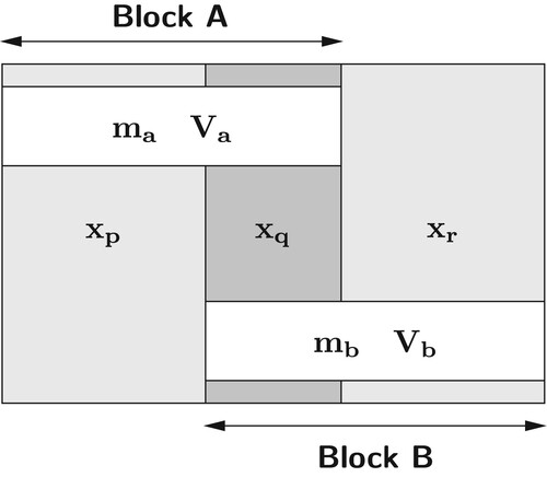
By way of example, Figure 1 shows a system of parameters and measurements partitioned into two blocks, A and B. Figure 2 illustrates a survey control network partitioned according to this scheme.

1. A system partitioned into two blocks.

2. A system of survey control measurements segmented into two blocks, Block A and Block B, with junction parameter stations identified in red.

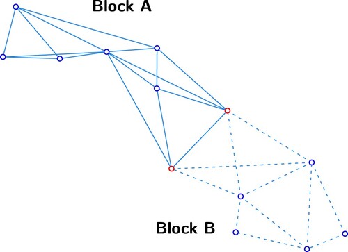
With reference to Figures 1 and 2, Block A is defined by the set of measurements ${\mathbf{m}}_{\mathbf{a}}$ with variance matrix ${\mathbf{V}}_{\mathbf{a}}$, and Block B is defined by the set of measurements ${\mathbf{m}}_{\mathbf{b}}$ with variance matrix ${\mathbf{V}}_{\mathbf{b}}$. ${\mathbf{x}}_{\mathbf{p}}$ contains the inner parameter stations in Block A and ${\mathbf{x}}_{\mathbf{r}}$ contains the inner parameter stations in Block B. ${\mathbf{x}}_{\mathbf{q}}$ represents the junction parameter stations which connect Blocks A and B through measurements ${\mathbf{m}}_{\mathbf{a}}$ and ${\mathbf{m}}_{\mathbf{b}}$. Fundamentally, a parameter station can only be regarded as inner if all measurements associated with it are contained within that block, whereas junction parameter stations are connected by measurements in two or more blocks. Hence, the parameter stations in ${\mathbf{x}}_{\mathbf{p}}$ and ${\mathbf{x}}_{\mathbf{r}}$ do not share any common measurements. Table 1 summarises the distribution of the parameters and measurements amongst the two blocks.

Table 1. Distribution of parameters and measurements of a simultaneous system segmented into two blocks.

With reference to Helmert's high-level instructions, Figure 3 shows the distribution of parameters in Table 1 in two levels, where Level 1 represents the ‘main system’ and Level 2 represents the partitioned blocks containing the ‘inner stations’.

3. Representation of Helmert blocks as a two-level system.

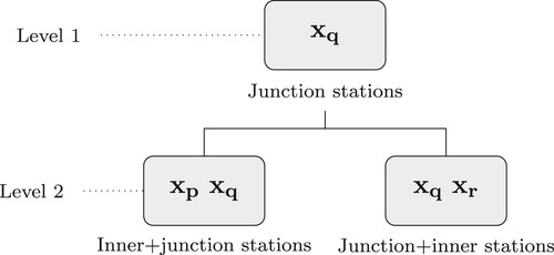
While this example shows only two levels and two blocks in the second level, the number of levels and/or blocks in each level may increase according to the way the network has been partitioned. Customary practice in this context has been to partition a network according to country or state boundaries; in rectangular regions defined by parallels and meridians; or by measurement type and quality (e.g. Hough 1948; Ehrnsperger 1991; Schwarz 1989; Pursell and Potterfield 2008).

2.1. Solution of parameters according to Helmert's method

Although Helmert did not provide theoretical development or proof for the estimation of parameter estimates according to his method, the derivation may be given as follows (c.f. Wolf 1978; Schwarz 1989; Leahy 1999; Teunissen 2003).

Using the partitioning scheme in Table 1, the observation equations and measurement variances can be generalised as (1) $\left[\begin{array}{c}{\mathbf{m}}_{\mathbf{a}}\\ {\mathbf{m}}_{\mathbf{b}}\end{array}\right]=\left[\begin{array}{ccc}{\mathbf{A}}_1& {\mathbf{A}}_2& \mathbf{0}\\ \mathbf{0}& {\mathbf{B}}_1& {\mathbf{B}}_2\end{array}\right]\left[\begin{array}{c}{\mathbf{x}}_{\mathbf{p}}\\ {\mathbf{x}}_{\mathbf{q}}\\ {\mathbf{x}}_{\mathbf{r}}\end{array}\right],{\mathbf{V}}_{\mathbf{m}}=\left[\begin{array}{cc}{\mathbf{V}}_{\mathbf{a}}& \mathbf{0}\\ \mathbf{0}& {\mathbf{V}}_{\mathbf{b}}\end{array}\right]$(1) From Equation (1(1) $\left[\begin{array}{c}{\mathbf{m}}_{\mathbf{a}}\\ {\mathbf{m}}_{\mathbf{b}}\end{array}\right]=\left[\begin{array}{ccc}{\mathbf{A}}_1& {\mathbf{A}}_2& \mathbf{0}\\ \mathbf{0}& {\mathbf{B}}_1& {\mathbf{B}}_2\end{array}\right]\left[\begin{array}{c}{\mathbf{x}}_{\mathbf{p}}\\ {\mathbf{x}}_{\mathbf{q}}\\ {\mathbf{x}}_{\mathbf{r}}\end{array}\right],{\mathbf{V}}_{\mathbf{m}}=\left[\begin{array}{cc}{\mathbf{V}}_{\mathbf{a}}& \mathbf{0}\\ \mathbf{0}& {\mathbf{V}}_{\mathbf{b}}\end{array}\right]$(1) ), the normal equations may be written as (2) $\left[\begin{array}{ccc}{\mathbf{N}}_{11}& {\mathbf{N}}_{12}& \mathbf{0}\\ {\mathbf{N}}_{21}& {\mathbf{N}}_{22}+{\mathbf{R}}_{11}& {\mathbf{R}}_{12}\\ \mathbf{0}& {\mathbf{R}}_{21}& {\mathbf{R}}_{22}\end{array}\right]\left[\begin{array}{c}{\hat{\mathbf{x}}}_{\mathbf{p}}\\ {\hat{\mathbf{x}}}_{\mathbf{q}}\\ {\hat{\mathbf{x}}}_{\mathbf{r}}\end{array}\right]=\left[\begin{array}{c}{\mathbf{N}}_1{\mathbf{m}}_{\mathbf{a}}\\ {\mathbf{N}}_2{\mathbf{m}}_{\mathbf{a}}+{\mathbf{R}}_1{\mathbf{m}}_{\mathbf{b}}\\ {\mathbf{R}}_2{\mathbf{m}}_{\mathbf{b}}\end{array}\right]$(2) where (3) $\begin{array}{cc}{\mathbf{N}}_{ij}& ={\mathbf{A}}_i^T{\mathbf{V}}_{\mathbf{a}}^{-1}{\mathbf{A}}_j,\mathrm{w}\mathrm{i}\mathrm{t}\mathrm{h}i=1\dots 2;j=1\dots 2\\ {\mathbf{N}}_i& ={\mathbf{A}}_i^T{\mathbf{V}}_{\mathbf{a}}^{-1},\mathrm{w}\mathrm{i}\mathrm{t}\mathrm{h}i=1\dots 2\\ {\mathbf{R}}_{ij}& ={\mathbf{B}}_i^T{\mathbf{V}}_{\mathbf{b}}^{-1}{\mathbf{B}}_j,\mathrm{w}\mathrm{i}\mathrm{t}\mathrm{h}i=1\dots 2;j=1\dots 2\\ {\mathbf{R}}_i& ={\mathbf{B}}_i^T{\mathbf{V}}_{\mathbf{b}}^{-1},\mathrm{w}\mathrm{i}\mathrm{t}\mathrm{h}i=1\dots 2.\end{array}$(3) After eliminating the inner unknowns ${\hat{\mathbf{x}}}_{\mathbf{p}}$ and ${\hat{\mathbf{x}}}_{\mathbf{r}}$ from the left-hand side of Equation (2(2) $\left[\begin{array}{ccc}{\mathbf{N}}_{11}& {\mathbf{N}}_{12}& \mathbf{0}\\ {\mathbf{N}}_{21}& {\mathbf{N}}_{22}+{\mathbf{R}}_{11}& {\mathbf{R}}_{12}\\ \mathbf{0}& {\mathbf{R}}_{21}& {\mathbf{R}}_{22}\end{array}\right]\left[\begin{array}{c}{\hat{\mathbf{x}}}_{\mathbf{p}}\\ {\hat{\mathbf{x}}}_{\mathbf{q}}\\ {\hat{\mathbf{x}}}_{\mathbf{r}}\end{array}\right]=\left[\begin{array}{c}{\mathbf{N}}_1{\mathbf{m}}_{\mathbf{a}}\\ {\mathbf{N}}_2{\mathbf{m}}_{\mathbf{a}}+{\mathbf{R}}_1{\mathbf{m}}_{\mathbf{b}}\\ {\mathbf{R}}_2{\mathbf{m}}_{\mathbf{b}}\end{array}\right]$(2) ), the reduced normal equations for the ‘main system’ (according to Helmert's high-level instructions) are $\begin{array}{rl}& \left[\begin{array}{ccc}{\mathbf{N}}_{11}& {\mathbf{N}}_{12}& \mathbf{0}\\ \mathbf{0}& {\overline{\mathbf{N}}}_{12}^T{\mathbf{V}}_{\mathbf{a}}^{-1}{\overline{\mathbf{N}}}_{12}+{\overline{\mathbf{R}}}_{21}^T{\mathbf{V}}_{\mathbf{b}}^{-1}{\overline{\mathbf{R}}}_{21}& \mathbf{0}\\ \mathbf{0}& {\mathbf{R}}_{21}& {\mathbf{R}}_{22}\end{array}\right]\left[\begin{array}{c}{\hat{\mathbf{x}}}_{\mathbf{p}}\\ {\hat{\mathbf{x}}}_{\mathbf{q}}\\ {\hat{\mathbf{x}}}_{\mathbf{r}}\end{array}\right]\\ \left(4\right)& & =\left[\begin{array}{c}{\mathbf{N}}_1{\mathbf{m}}_{\mathbf{a}}\\ {\overline{\mathbf{N}}}_{12}^T{\mathbf{V}}_{\mathbf{a}}^{-1}{\mathbf{m}}_{\mathbf{a}}+{\overline{\mathbf{R}}}_{21}^T{\mathbf{V}}_{\mathbf{b}}^{-1}{\mathbf{m}}_{\mathbf{b}}\\ {\mathbf{R}}_2{\mathbf{m}}_{\mathbf{b}}\end{array}\right]\end{array}$where (5) ${\overline{\mathbf{N}}}_{12}=[\mathbf{I}-{\mathbf{A}}_1({\mathbf{N}}_{11}{)}^{-1}{\mathbf{N}}_1]{\mathbf{A}}_2$(5) (6) ${\overline{\mathbf{R}}}_{21}=[\mathbf{I}-{\mathbf{B}}_2({\mathbf{R}}_{22}{)}^{-1}{\mathbf{R}}_2]{\mathbf{B}}_1.$(6) Therefore, the solution of the junction station parameter estimates ${\hat{\mathbf{x}}}_{\mathbf{q}}$ of the main system (i.e. Level 1) can be expressed as (7) $\begin{array}{rll}{\hat{\mathbf{x}}}_{\mathbf{q}}& ={[{\overline{\mathbf{N}}}_{12}^T{\mathbf{V}}_{\mathbf{a}}^{-1}{\overline{\mathbf{N}}}_{12}+{\overline{\mathbf{R}}}_{21}^T{\mathbf{V}}_{\mathbf{b}}^{-1}{\overline{\mathbf{R}}}_{21}]}^{-1}& \\ & \times [{\overline{\mathbf{N}}}_{12}^T{\mathbf{V}}_{\mathbf{a}}^{-1}{\mathbf{m}}_{\mathbf{a}}+{\overline{\mathbf{R}}}_{21}^T{\mathbf{V}}_{\mathbf{b}}^{-1}{\mathbf{m}}_{\mathbf{b}}].\end{array}$(7) By substituting ${\hat{\mathbf{x}}}_{\mathbf{q}}$ into the first and third sets of normal equations in Equation (4$\begin{array}{rl}& \left[\begin{array}{ccc}{\mathbf{N}}_{11}& {\mathbf{N}}_{12}& \mathbf{0}\\ \mathbf{0}& {\overline{\mathbf{N}}}_{12}^T{\mathbf{V}}_{\mathbf{a}}^{-1}{\overline{\mathbf{N}}}_{12}+{\overline{\mathbf{R}}}_{21}^T{\mathbf{V}}_{\mathbf{b}}^{-1}{\overline{\mathbf{R}}}_{21}& \mathbf{0}\\ \mathbf{0}& {\mathbf{R}}_{21}& {\mathbf{R}}_{22}\end{array}\right]\left[\begin{array}{c}{\hat{\mathbf{x}}}_{\mathbf{p}}\\ {\hat{\mathbf{x}}}_{\mathbf{q}}\\ {\hat{\mathbf{x}}}_{\mathbf{r}}\end{array}\right]\\ \left(4\right)& & =\left[\begin{array}{c}{\mathbf{N}}_1{\mathbf{m}}_{\mathbf{a}}\\ {\overline{\mathbf{N}}}_{12}^T{\mathbf{V}}_{\mathbf{a}}^{-1}{\mathbf{m}}_{\mathbf{a}}+{\overline{\mathbf{R}}}_{21}^T{\mathbf{V}}_{\mathbf{b}}^{-1}{\mathbf{m}}_{\mathbf{b}}\\ {\mathbf{R}}_2{\mathbf{m}}_{\mathbf{b}}\end{array}\right]\end{array}$), the inner station parameter estimates ${\hat{\mathbf{x}}}_{\mathbf{p}}$ and ${\hat{\mathbf{x}}}_{\mathbf{r}}$ (i.e. Level 2) can be solved as (c.f. Equation 3(3) $\begin{array}{cc}{\mathbf{N}}_{ij}& ={\mathbf{A}}_i^T{\mathbf{V}}_{\mathbf{a}}^{-1}{\mathbf{A}}_j,\mathrm{w}\mathrm{i}\mathrm{t}\mathrm{h}i=1\dots 2;j=1\dots 2\\ {\mathbf{N}}_i& ={\mathbf{A}}_i^T{\mathbf{V}}_{\mathbf{a}}^{-1},\mathrm{w}\mathrm{i}\mathrm{t}\mathrm{h}i=1\dots 2\\ {\mathbf{R}}_{ij}& ={\mathbf{B}}_i^T{\mathbf{V}}_{\mathbf{b}}^{-1}{\mathbf{B}}_j,\mathrm{w}\mathrm{i}\mathrm{t}\mathrm{h}i=1\dots 2;j=1\dots 2\\ {\mathbf{R}}_i& ={\mathbf{B}}_i^T{\mathbf{V}}_{\mathbf{b}}^{-1},\mathrm{w}\mathrm{i}\mathrm{t}\mathrm{h}i=1\dots 2.\end{array}$(3) ) (8) ${\hat{\mathbf{x}}}_{\mathbf{p}}=({\mathbf{N}}_{11}{)}^{-1}{\mathbf{N}}_1[{\mathbf{m}}_{\mathbf{a}}-{\mathbf{A}}_2{\hat{\mathbf{x}}}_{\mathbf{q}}]$(8) (9) ${\hat{\mathbf{x}}}_{\mathbf{r}}=({\mathbf{R}}_{22}{)}^{-1}{\mathbf{R}}_2[{\mathbf{m}}_{\mathbf{b}}-{\mathbf{B}}_1{\hat{\mathbf{x}}}_{\mathbf{q}}]$(9) with variance matrices for ${\hat{\mathbf{x}}}_{\mathbf{q}}$, ${\hat{\mathbf{x}}}_{\mathbf{p}}$ and ${\hat{\mathbf{x}}}_{\mathbf{r}}$ being (10) ${\mathbf{V}}_{{\hat{\mathbf{x}}}_{\mathbf{q}}}={[{\overline{\mathbf{N}}}_{12}^T{\mathbf{V}}_{\mathbf{a}}^{-1}{\overline{\mathbf{N}}}_{12}+{\overline{\mathbf{R}}}_{21}^T{\mathbf{V}}_{\mathbf{b}}^{-1}{\overline{\mathbf{R}}}_{21}]}^{-1}$(10) (11) $\begin{array}{rll}{\mathbf{V}}_{{\hat{\mathbf{x}}}_{\mathbf{p}}}& =\left[\right({\mathbf{N}}_{11}{)}^{-1}{\mathbf{A}}_1^T{\mathbf{V}}_{\mathbf{a}}^{-1}][{\mathbf{V}}_{\mathbf{a}}^{-1}+{\mathbf{A}}_2{\mathbf{V}}_{{\hat{\mathbf{x}}}_{\mathbf{q}}}{\mathbf{A}}_2^T]& \\ & \times {\left[\right({\mathbf{N}}_{11}{)}^{-1}{\mathbf{A}}_1^T{\mathbf{V}}_{\mathbf{a}}^{-1}]}^T\end{array}$(11) (12) $\begin{array}{rll}{\mathbf{V}}_{{\hat{\mathbf{x}}}_{\mathbf{r}}}& =\left[\right({\mathbf{R}}_{22}{)}^{-1}{\mathbf{B}}_1^T{\mathbf{V}}_{\mathbf{b}}^{-1}][{\mathbf{V}}_{\mathbf{b}}^{-1}+{\mathbf{B}}_2{\mathbf{V}}_{{\hat{\mathbf{x}}}_{\mathbf{q}}}{\mathbf{B}}_2^T]& \\ & \times {\left[\right({\mathbf{R}}_{22}{)}^{-1}{\mathbf{B}}_1^T{\mathbf{V}}_{\mathbf{b}}^{-1}]}^T.\end{array}$(12) In practice, the system is often solved in reverse, working from lower level blocks up to the highest, and then via back-substitution down to lower blocks. Under this approach, the normal equations for blocks A and B in Level 2 are reduced independently first, and then combined to solve the junctions stations in Level 1. That is, after independently reducing the normal equations for blocks A and B, the two reduced normal blocks ${\overline{\mathbf{N}}}_{12}^T{\mathbf{V}}_{\mathbf{a}}^{-1}{\overline{\mathbf{N}}}_{12}$ and ${\overline{\mathbf{R}}}_{21}^T{\mathbf{V}}_{\mathbf{b}}^{-1}{\overline{\mathbf{R}}}_{21}$, and the two reduced measurement vectors ${\overline{\mathbf{N}}}_{12}^T{\mathbf{V}}_{\mathbf{a}}^{-1}{\mathbf{m}}_{\mathbf{a}}$ and ${\overline{\mathbf{R}}}_{21}^T{\mathbf{V}}_{\mathbf{b}}^{-1}{\mathbf{m}}_{\mathbf{b}}$ are combined in Equation (7(7) $\begin{array}{rll}{\hat{\mathbf{x}}}_{\mathbf{q}}& ={[{\overline{\mathbf{N}}}_{12}^T{\mathbf{V}}_{\mathbf{a}}^{-1}{\overline{\mathbf{N}}}_{12}+{\overline{\mathbf{R}}}_{21}^T{\mathbf{V}}_{\mathbf{b}}^{-1}{\overline{\mathbf{R}}}_{21}]}^{-1}& \\ & \times [{\overline{\mathbf{N}}}_{12}^T{\mathbf{V}}_{\mathbf{a}}^{-1}{\mathbf{m}}_{\mathbf{a}}+{\overline{\mathbf{R}}}_{21}^T{\mathbf{V}}_{\mathbf{b}}^{-1}{\mathbf{m}}_{\mathbf{b}}].\end{array}$(7) ) to estimate the station parameters ${\hat{\mathbf{x}}}_{\mathbf{q}}$ of the main system. Back-substitution is then undertaken to produce estimates for the station parameters ${\hat{\mathbf{x}}}_{\mathbf{p}}$ and ${\hat{\mathbf{x}}}_{\mathbf{r}}$ of lower blocks using Equations (8(8) ${\hat{\mathbf{x}}}_{\mathbf{p}}=({\mathbf{N}}_{11}{)}^{-1}{\mathbf{N}}_1[{\mathbf{m}}_{\mathbf{a}}-{\mathbf{A}}_2{\hat{\mathbf{x}}}_{\mathbf{q}}]$(8) ) and (9(9) ${\hat{\mathbf{x}}}_{\mathbf{r}}=({\mathbf{R}}_{22}{)}^{-1}{\mathbf{R}}_2[{\mathbf{m}}_{\mathbf{b}}-{\mathbf{B}}_1{\hat{\mathbf{x}}}_{\mathbf{q}}]$(9) ). This may be repeated for as many iterations as required.

In cases where, for example, geodetic networks pertaining to blocks A and B are maintained by different countries whose policies prevent making data openly accessible, a practical benefit of this approach is the ability for participating organisations to obtain local station parameter estimates from the junction station estimates (computed by a central agency) without ever having to disclose their raw measurements or station coordinates (Teunissen 2003).

2.2. Variations of Helmert blocking

Helmert blocking, in principle, has been used extensively over the last century to estimate parameters for large geodetic networks, which would otherwise be unattainable if approached using a simultaneous solution. However, not all adjustments which have employed Helmert's method of partitioning a network adjustment into smaller parts truly reflect Helmert's high-level instructions (c.f. Section 2) for solving the unknowns. In some cases, practical convenience or customary practice has led to non-rigorous results. The reasons for this are varied and most commonly stem from the inordinate computational burden of reducing large sets of normal equations, eliminating equations for the inner stations and estimating the unknowns. Common variations of Helmert's method include:

The Bowie method. This method was developed by Adams (1930) and employed for the establishment of the North American Datum of 1927 (NAD27). As described by Schwarz (1989) and Dracup (1989), the Bowie method is ‘a modified Helmert block adjustment’ that yields an approximate solution of the station coordinates. There are several reasons for this, the most notable of which are as follows.

• Once the network is segmented into junctions and segments (i.e. two levels), all base lines and azimuths between junction stations computed from (Laplace) latitude and longitude observations at the junction stations are held fixed.

• All directions relating to the junction stations are equally weighted.

• All off-diagonal terms in the normal equations relating to junction parameters are ignored.

• Junction parameters are held fixed in the solution of the inner stations within each Helmert block.

Given the computing capabilities of the time, the method provided a most pragmatic solution to what was for the time an overwhelming computational challenge.

Modified Bowie method. Recognising the weaknesses of the Bowie method, advancements on the method have been undertaken on different occasions and with different improvements. Notable applications include the establishment of the European Datum 1950 (ED50) (Hough 1948; Wolf 1978) and the Australian Geodetic Datum 1966 (AGD66) (Bomford 1967). In both cases, however, procedures involving the use of condition equations with artificial constraints and holding junction stations fixed were employed. While modifications to the procedures for establishing the junction station estimates yielded overall improvements in accuracy, the final results were not consistent with that which would have otherwise been produced from a simultaneous solution.

Canadian Section method. This method was developed by Pinch and Peterson (1974) and was used for the Geodetic Model of Australia adjustments (GMA73, GMA80, GMA82, GMA84) that led to the establishment of the Australian Geodetic Datum 1984 (AGD84) (Allman and Steed 1980; Allman 1983; Allman and Veenstra 1984). It was also used for the national adjustment that produced the Geodetic Datum of Australia (GDA94) (Steed and Allman 2005). This method adopts the principles of Helmert blocking, however, is unable to provide for rigorous variance matrices for all stations as it involves fixing junction station estimates when estimating the inner stations in the back-substitution step (Pinch and Peterson 1974; Gagnon 1976; Golub and Plemmons 1980; Golub et al. 1988; Snay 1990; Leahy and Collier 1998; Leahy 1999; Steed and Allman 2005). The other aspect that needs to be kept in mind is that in some cases (e.g. Allman and Veenstra 1984; Steed and Allman 2005), the constraint stations used to propagate datum into an adjustment are held fixed, which in turn weakens the quality of the estimated station coordinates and their variance matrices.

Helmert–Wolf method. This method was developed by Wolf (1978) for the adjustment for the North American Datum 1983 (NAD 83) (Stoughton 1989; Pursell and Potterfield 2008) and has been used extensively in modern geodetic adjustments. Notable applications include the readjustment of the European Triangulation network (RETrig) for the establishment of the European Datum 1987 (ED87) (Ehrnsperger 1991); the adjustment of the South American Geocentric Reference System (SIRGAS) (Costa et al. 1998; Fortes 1998); and the subsequent re-adjustments of NAD 83 (2007 and 2011) (Pursell and Potterfield 2008; Dennis 2020).

In theory, the method of Helmert blocking offers the potential for producing rigorous estimates for station coordinates and variances. Provided the data has been partitioned and organised according to a scheme that respects the sparsity of the observation equations, the method can also offer a very fast approach to solving station coordinate estimates via parallel Cholesky decomposition (or factorisation) and back-substitution (Avila and Tomlin 1979). However, if the back-substitution to lower blocks is not undertaken correctly, non-rigorous estimates will result. For instance, incorrectly passing variances estimated for the highest level block into lower blocks can have the same effect as introducing measurement contributions twice, yielding more optimistic variances than would be achieved using a simultaneous solution. This effect will be observed by increasing precisions on each adjustment iteration.

2.3. Limitations of traditional, rigid Helmert blocking structures

While the principle of Helmert blocking offers immediate efficiency gains over a simultaneous approach, the traditional way in which a network is partitioned to satisfy the method of Helmert blocking can introduce unintentional consequences for, and practical limitations to maintaining large and continually updated geodetic networks. In addition, depending on how the size, connectivity, and composition of the network has grown over time, it may not be practically feasible to solve the entire network via a single system of blocks using the Helmert blocking method (e.g. Pursell and Potterfield 2008; Dennis 2020).

The premise behind successful Helmert blocking adjustments assumes that the system of normal equations is either sparse or can be divided into logical blocks such that connecting measurements and correlations do not exist between the lower-level blocks (Golub and Plemmons 1980; Meissl 1980). A limitation that has arisen with the use of Helmert blocking is that networks are often subdivided and maintained using rigid, hierarchical block structures, delineated by geographical boundaries or by measurement type. This may have been a characteristic feature of geodetic networks in the nineteenth and mid-twentieth centuries, or when it has not been possible, practically or politically, to share data across jurisdictional boundaries. With the rapid expansion of geodetic networks over the last 50 years, geodetic networks are rarely developed in such a way that affords simple delineation or configuration into logical or geographical blocks.

If a rigid block partitioning structure has been chosen, the extent to which the least squares solution can adapt to the changing state of the network will be limited. Although a geodetic network may have been previously subdivided into conveniently shaped blocks which do not have connecting measurements between them, they are almost impossible to maintain in this way with ongoing geodetic network maintenance and the requirement to install new control marks for infrastructure projects. Since introducing new measurements can potentially introduce new correlations between blocks or radically change the sparsity by which the observation equations have been ordered, either the block partitions must be re-configured or the correlations be dealt with another way. To address this issue, common approaches can include one or more of the following:

• Partition the network into blocks characterised by measurement type (GNSS/terrestrial; 3D/2D)

• Maintain specific networks according to measurement fidelity (e.g. high-precision fiducial networks, lower quality subsidiary networks). Parameter estimates for the fiducial network are solved independently and then introduced as constraints to subsidiary networks

• Retain rigid block partitions and then execute measurement campaigns according to those blocks

• Employ complex decorrelation algorithms, which is theoretically possible but practically challenging and inconvenient for very large systems of measurements.

Given the shortcomings of traditional rigid blocking approaches, there is a strong need for a more adaptive, flexible and automated approach to the way in which a network is partitioned and adjusted such that the constantly changing nature of present-day geodetic networks can be updated in an efficient, yet fully rigorous manner.

Tienstra's method of solving parameters in phases does not limit the way in which a network can be subdivided, nor does it prohibit the solution of blocks having junction stations with no connecting measurements to the inner stations. Neither does it impose the need for hierarchical block structures. As will be explained in Section 3, Tienstra's method affords a rigorous solution while at the same time, offers tremendous flexibility and versatility unavailable with traditional approaches. However, to realise the benefits of Tienstra's method for large geodetic networks subject to continual change, an adaptive segmentation algorithm is required. This will be dealt with in Section 4.

3. Review of Tienstra's phased least squares method

In this section, we review Tienstra's method for estimating parameters and their variances in phases. We then compare it with the method for estimating a partial set of parameters from a (total) simultaneous solution to demonstrate that Tienstra's method is identical to that which would be derived from a simultaneous solution of the entire network, proving that the strategy is entirely rigorous. This is important as it means the same results will be achieved (as the simultaneous solution) irrespective of the way the network has been segmented.

3.1. Tienstra's method of adjustment in phases

Tienstra's phased least squares algorithm was published and implemented posthumously (1956; 1963), and has been reviewed by several authors (Lambeck 1963; Baarda 1967; Krakiwsky 1975; Cooper and Leahy 1977; Leahy 1983; Leahy et al. 1986; Leahy and Collier 1998; Teunissen 2003). A detailed summary of the variations between Tienstra's method and other sequential least squares methods is provided by Krakiwsky (1975). Conceptually, the method is executed in a sequential fashion similar to that of smoothing filters (e.g. Kalman filter, fixed-interval smoothing). The main distinction is that forward, backward and combination passes are required if all parameters and their variances are to be solved, so as to ensure all available data contributes to each parameter in a rigorous way. If the latest parameters for a subset of the network is required, then the system of blocks can be configured such that only a single pass is required.

Mathematically, it is equivalent to the method of stacking normal equations developed by Krüger (1905) and the algorithm developed by Schmid and Schmid (1965) for solving least squares problems sequentially (Lambeck 1963; Kouba 1970; Chung-Chi 1970; Kouba 1972; Krakiwsky 1975). Fundamental contributions to the method have been made by Kouba (1970), Chung-Chi (1970), Kouba (1972) and Collier and Leahy (1992). It also forms the basis of work to develop an automatic procedure for segmenting a network and a rigorous approach for the extension and integration of networks over time (Leahy 1999). One of the goals of this contribution is to show how simple, flexible, versatile and elegant Tienstra's method is for solving problems of almost any size, provided there is at hand an automatic way to segment the measurements in blocks irrespective of the sparseness of the normal equations, the distribution and extent of correlated measurements, or how often measurements are added or removed.

Assuming a network has been partitioned into a sequential list of blocks where all the junction stations of each block are shared only with those of the next block in the sequence (according to certain prerequisite features, c.f. Section 4), Tienstra's method can be implemented using the following high-level steps (Tienstra 1956):

(1)	Commencing with the first block, solve the parameter estimates and variances for each block in succession via a forward pass
(2)	Upon the solution of each block, introduce the junction parameter estimates and variances to the next block as measurements and solve. Repeat until the last block in the sequence is solved. The estimates and variances for all stations in the last block will be rigorous.
(3)	Commencing with the last block, solve the parameter estimates and variances for each block in succession via a reverse pass.
(4)	As with (2) but in reverse, junction parameter estimates and variances solved for each block are passed to the next block until the first block in the sequence is solved. The estimates and variances for all stations in the first block will be rigorous.
(5)	For each intermediate block (i.e. not the first or last), integrate junction parameter estimates and variances from previous and following blocks. At this point, the estimates and variances for all stations in this block will be rigorous. This step is repeated for as many intermediate blocks as required.

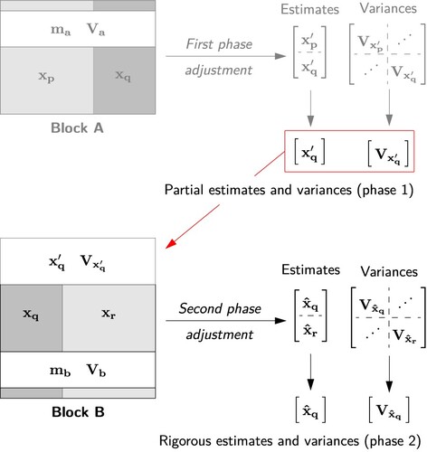
With reference to the segmented network in Figure 1 and distribution of parameters and measurements in Table 1, the theoretical development for Tienstra's method is given as follows. In this development, the passing of junction parameter estimates solved in one block to the next block, as per steps (2) and (4), is explained in terms of ‘first phase’ and ‘second phase’ adjustments.

3.1.1. First phase

Figure 4 illustrates the solution of segmented Block A and generation of estimates ${\mathbf{x}}_{\mathbf{p}}^{\prime }$ and ${\mathbf{x}}_{\mathbf{q}}^{\prime }$ and the full variance matrix ${\mathbf{V}}_{{\mathbf{x}}_{\mathbf{p}\mathbf{q}}^{\prime }}$ through a first phase solution. The estimates ${\mathbf{x}}_{\mathbf{q}}^{\prime }$ and variance matrix ${\mathbf{V}}_{{\mathbf{x}}_{\mathbf{q}}^{\prime }}$ are those of the junction parameters which are passed to the second phase solution.

4. Solution of junction parameter estimates via first phase adjustment.

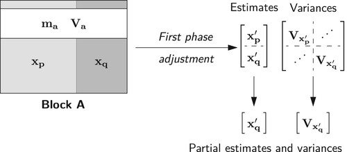
In the first phase solution, Block A is adjusted using measurements ${\mathbf{m}}_{\mathbf{a}}$ only, the observation equations for which are: (13) $\left[\begin{array}{cc}{\mathbf{A}}_1& {\mathbf{A}}_2\end{array}\right]\left[\begin{array}{c}{\mathbf{x}}_{\mathbf{p}}\\ {\mathbf{x}}_{\mathbf{q}}\end{array}\right]=\left[\begin{array}{c}{\mathbf{m}}_{\mathbf{a}}\end{array}\right]$(13) From Equation (13(13) $\left[\begin{array}{cc}{\mathbf{A}}_1& {\mathbf{A}}_2\end{array}\right]\left[\begin{array}{c}{\mathbf{x}}_{\mathbf{p}}\\ {\mathbf{x}}_{\mathbf{q}}\end{array}\right]=\left[\begin{array}{c}{\mathbf{m}}_{\mathbf{a}}\end{array}\right]$(13) ), the complete first phase estimates can be expressed as (14) $\left[\begin{array}{c}{\mathbf{x}}_{\mathbf{p}}^{\prime }\\ ---\\ {\mathbf{x}}_{\mathbf{q}}^{\prime }\end{array}\right]={\left[\begin{array}{c}{\mathbf{C}}_{11}\genfrac{}{}{0ex}{}{|}{|}{\mathbf{C}}_{12}\\ ------\\ {\mathbf{C}}_{21}\genfrac{}{}{0ex}{}{|}{|}{\mathbf{C}}_{22}\end{array}\right]}^{-1}\left[\begin{array}{c}{\mathbf{C}}_1\\ ---\\ {\mathbf{C}}_2\end{array}\right]\left[\begin{array}{c}{\mathbf{m}}_{\mathbf{a}}\end{array}\right],$(14) where (15) $\begin{array}{cc}{\mathbf{C}}_{ij}& ={\mathbf{A}}_i^T{\mathbf{V}}_{\mathbf{a}}^{-1}{\mathbf{A}}_j,\mathrm{w}\mathrm{i}\mathrm{t}\mathrm{h}i=1\dots 2;j=1\dots 2\\ {\mathbf{C}}_i& ={\mathbf{A}}_i^T{\mathbf{V}}_{\mathbf{a}}^{-1},\mathrm{w}\mathrm{i}\mathrm{t}\mathrm{h}i=1\dots 2.\end{array}$(15) From Equation (14(14) $\left[\begin{array}{c}{\mathbf{x}}_{\mathbf{p}}^{\prime }\\ ---\\ {\mathbf{x}}_{\mathbf{q}}^{\prime }\end{array}\right]={\left[\begin{array}{c}{\mathbf{C}}_{11}\genfrac{}{}{0ex}{}{|}{|}{\mathbf{C}}_{12}\\ ------\\ {\mathbf{C}}_{21}\genfrac{}{}{0ex}{}{|}{|}{\mathbf{C}}_{22}\end{array}\right]}^{-1}\left[\begin{array}{c}{\mathbf{C}}_1\\ ---\\ {\mathbf{C}}_2\end{array}\right]\left[\begin{array}{c}{\mathbf{m}}_{\mathbf{a}}\end{array}\right],$(14) ), the variance matrix of the estimates ${\mathbf{x}}_{\mathbf{p}}^{\prime }$ and ${\mathbf{x}}_{\mathbf{q}}^{\prime }$ is (16) ${\left[\begin{array}{c}{\mathbf{C}}_{11}\genfrac{}{}{0ex}{}{|}{|}{\mathbf{C}}_{12}\\ ------\\ {\mathbf{C}}_{21}\genfrac{}{}{0ex}{}{|}{|}{\mathbf{C}}_{22}\end{array}\right]}^{-1}.$(16) Here, it is assumed that the inverse of the normal matrix can be taken. In practice, this will be true if sufficient parameter constraints and connections to datum are available in each block of the segmented network. In the case of rank deficiency caused by a lack of measurements in a segmented block, it will be necessary to impose large variances to stations without sufficient connections to datum so that the normal matrices associated with a block will always be non-singular. Leahy (1999) shows that this can be done in a manner that does not bias the final estimates beyond a statistically negligible level.

As the matrix in Equation (16(16) ${\left[\begin{array}{c}{\mathbf{C}}_{11}\genfrac{}{}{0ex}{}{|}{|}{\mathbf{C}}_{12}\\ ------\\ {\mathbf{C}}_{21}\genfrac{}{}{0ex}{}{|}{|}{\mathbf{C}}_{22}\end{array}\right]}^{-1}.$(16) ) is the variance matrix of the estimates $[{\mathbf{x}}_{\mathbf{p}}^{\prime }{\mathbf{x}}_{\mathbf{q}}^{\prime }{]}^T$, the lower right-hand element ${\mathbf{C}}_{22}$ represents the variance matrix ${\mathbf{V}}_{{\mathbf{x}}_{\mathbf{q}}^{\prime }}$ of the junction parameter estimates ${\mathbf{x}}_{\mathbf{q}}^{\prime }$.

Using Equation (A3(A3) ${\mathbf{E}}_{22}={[{\mathbf{E}}_{22}-{\mathbf{E}}_{21}{\mathbf{E}}_{11}^{-1}{\mathbf{E}}_{12}]}^{-1}$(A3) ) in Appendix A.1, to which we refer for the full derivations of the partitioned model, the lower partition of variance matrix ${\mathbf{V}}_{{\mathbf{x}}_{\mathbf{q}}^{\prime }}$ can be expressed as (17) ${\mathbf{V}}_{{\mathbf{x}}_{\mathbf{q}}^{\prime }}={[{\mathbf{C}}_{22}-{\mathbf{C}}_{21}{\mathbf{C}}_{11}^{-1}{\mathbf{C}}_{12}]}^{-1}.$(17) Taking the partial solution (using Equation (A13(A13) ${\mathbf{x}}_2=[-{[{\mathbf{E}}_{22}-{\mathbf{E}}_{21}{\mathbf{E}}_{11}^{-1}{\mathbf{E}}_{12}]}^{-1}]\left[\begin{array}{cc}{\mathbf{E}}_{21}{\mathbf{E}}_{11}^{-1}& \mathbf{I}\end{array}\right]\left[\begin{array}{c}{\mathbf{y}}_1\\ {\mathbf{y}}_2\end{array}\right].$(A13) ) in Appendix A.2) and substituting Equation (17(17) ${\mathbf{V}}_{{\mathbf{x}}_{\mathbf{q}}^{\prime }}={[{\mathbf{C}}_{22}-{\mathbf{C}}_{21}{\mathbf{C}}_{11}^{-1}{\mathbf{C}}_{12}]}^{-1}.$(17) ), junction parameter estimates ${\mathbf{x}}_{\mathbf{q}}^{\prime }$ can be simplified as (18) ${\mathbf{x}}_{\mathbf{q}}^{\prime }={\mathbf{V}}_{{\mathbf{x}}_{\mathbf{q}}^{\prime }}[-{\mathbf{C}}_{21}{\mathbf{C}}_{11}^{-1}{\mathbf{C}}_1+{\mathbf{C}}_2]\left[{\mathbf{m}}_{\mathbf{a}}\right].$(18)

3.1.2. Second phase

Figure 5 illustrates the rigorous solution of ${\hat{\mathbf{x}}}_{\mathbf{q}}$ and ${\hat{\mathbf{x}}}_{\mathbf{r}}$ in Block B through a second phase solution. For this phase, the partial estimates and variances from the first phase solution (denoted as ${\mathbf{x}}_{\mathbf{q}}^{\prime }$ and ${\mathbf{V}}_{{\mathbf{x}}_{\mathbf{q}}^{\prime }}$ in Equations (18(18) ${\mathbf{x}}_{\mathbf{q}}^{\prime }={\mathbf{V}}_{{\mathbf{x}}_{\mathbf{q}}^{\prime }}[-{\mathbf{C}}_{21}{\mathbf{C}}_{11}^{-1}{\mathbf{C}}_1+{\mathbf{C}}_2]\left[{\mathbf{m}}_{\mathbf{a}}\right].$(18) ) and (17(17) ${\mathbf{V}}_{{\mathbf{x}}_{\mathbf{q}}^{\prime }}={[{\mathbf{C}}_{22}-{\mathbf{C}}_{21}{\mathbf{C}}_{11}^{-1}{\mathbf{C}}_{12}]}^{-1}.$(17) ) respectively) are integrated with the measurements of Block B.

5. Solution of parameter estimates via second phase adjustment.

The observation equations for a second phase solution are (19) $\left[\begin{array}{cc}\mathbf{I}& \mathbf{0}\\ {\mathbf{B}}_1& {\mathbf{B}}_2\end{array}\right]\left[\begin{array}{c}{\mathbf{x}}_{\mathbf{q}}\\ {\mathbf{x}}_{\mathbf{r}}\end{array}\right]=\left[\begin{array}{c}{\mathbf{x}}_{\mathbf{q}}^{\prime }\\ {\mathbf{m}}_{\mathbf{b}}\end{array}\right],$(19) which, after substituting Equation (18(18) ${\mathbf{x}}_{\mathbf{q}}^{\prime }={\mathbf{V}}_{{\mathbf{x}}_{\mathbf{q}}^{\prime }}[-{\mathbf{C}}_{21}{\mathbf{C}}_{11}^{-1}{\mathbf{C}}_1+{\mathbf{C}}_2]\left[{\mathbf{m}}_{\mathbf{a}}\right].$(18) ) for ${\mathbf{x}}_{\mathbf{q}}^{\prime }$ from the first phase solution, take the form: (20) $\left[\begin{array}{cc}\mathbf{I}& \mathbf{0}\\ {\mathbf{B}}_1& {\mathbf{B}}_2\end{array}\right]\left[\begin{array}{c}{\mathbf{x}}_{\mathbf{q}}\\ {\mathbf{x}}_{\mathbf{r}}\end{array}\right]=\left[\begin{array}{cc}{\mathbf{V}}_{{{\mathbf{x}}^{\mathrm{\prime }}}_{\mathbf{q}}}\left[-{\mathbf{C}}_{21}{\mathbf{C}}_{11}^{-1}{\mathbf{C}}_1+{\mathbf{C}}_2\right]& \mathbf{0}\\ \mathbf{0}& \mathbf{I}\end{array}\right]\left[\begin{array}{c}{\mathbf{m}}_{\mathbf{a}}\\ {\mathbf{m}}_{\mathbf{b}}\end{array}\right].$(20) As the set of measurements $[{\mathbf{x}}_{\mathbf{q}}^{\prime }{\mathbf{m}}_{\mathbf{b}}{]}^T$ has the variance matrix $\lfloor \begin{array}{cc}{\mathbf{V}}_{{\mathbf{x}}_{\mathbf{q}}^{\prime }}& \mathbf{0}\\ \mathbf{0}& {\mathbf{V}}_{\mathbf{b}}\end{array}\rfloor$, the normal equations can be expressed as (21) $\left[\begin{array}{cc}{\mathbf{V}}_{{\mathbf{x}}_{\mathbf{q}}^{\prime }}^{-1}+{\mathbf{D}}_{11}& {\mathbf{D}}_{12}\\ {\mathbf{D}}_{21}& {\mathbf{D}}_{22}\end{array}\right]\left[\begin{array}{c}{\mathbf{x}}_{\mathbf{q}}\\ {\mathbf{x}}_{\mathbf{r}}\end{array}\right]=\left[\begin{array}{cc}-{\mathbf{C}}_{21}{\mathbf{C}}_{11}^{-1}{\mathbf{C}}_1+{\mathbf{C}}_2& {\mathbf{D}}_1\\ \mathbf{0}& {\mathbf{D}}_2\end{array}\right]\left[\begin{array}{c}{\mathbf{m}}_{\mathbf{a}}\\ {\mathbf{m}}_{\mathbf{b}}\end{array}\right],$(21) where (22) $\begin{array}{rl}{\mathbf{D}}_{ij}& ={\mathbf{B}}_i^T{\mathbf{V}}_{\mathbf{b}}^{-1}{\mathbf{B}}_j,\mathrm{w}\mathrm{i}\mathrm{t}\mathrm{h}i=1\dots 2;j=1\dots 2\\ {\mathbf{D}}_i& ={\mathbf{B}}_i^T{\mathbf{V}}_{\mathbf{b}}^{-1},\mathrm{w}\mathrm{i}\mathrm{t}\mathrm{h}i=1\dots 2.\end{array}$(22) Substituting Equation (17(17) ${\mathbf{V}}_{{\mathbf{x}}_{\mathbf{q}}^{\prime }}={[{\mathbf{C}}_{22}-{\mathbf{C}}_{21}{\mathbf{C}}_{11}^{-1}{\mathbf{C}}_{12}]}^{-1}.$(17) ) for ${\mathbf{V}}_{{\mathbf{x}}_{\mathbf{q}}^{\prime }}^{-1}$, the second phase estimate for the parameters ${\mathbf{x}}_{\mathbf{q}}$ and ${\mathbf{x}}_{\mathbf{r}}$ can be written as (23) $\begin{array}{rl}\left[\begin{array}{c}{\hat{\mathbf{x}}}_{\mathbf{q}}\\ {\hat{\mathbf{x}}}_{\mathbf{r}}\end{array}\right]& ={\left[\begin{array}{cc}{\mathbf{C}}_{22}-{\mathbf{C}}_{21}{\mathbf{C}}_{11}^{-1}{\mathbf{C}}_{12}+{\mathbf{D}}_{11}& {\mathbf{D}}_{12}\\ {\mathbf{D}}_{21}& {\mathbf{D}}_{22}\end{array}\right]}^{-1}\\ & \times \left[\begin{array}{cc}-{\mathbf{C}}_{21}{\mathbf{C}}_{11}^{-1}{\mathbf{C}}_1+{\mathbf{C}}_2& {\mathbf{D}}_1\\ \mathbf{0}& {\mathbf{D}}_2\end{array}\right]\left[\begin{array}{c}{\mathbf{m}}_{\mathbf{a}}\\ {\mathbf{m}}_{\mathbf{b}}\end{array}\right].\end{array}$(23) In Section 3.2, it will be shown that the estimates for $[{\hat{\mathbf{x}}}_{\mathbf{q}}{\hat{\mathbf{x}}}_{\mathbf{r}}{]}^T$ in Equation (23(23) $\begin{array}{rl}\left[\begin{array}{c}{\hat{\mathbf{x}}}_{\mathbf{q}}\\ {\hat{\mathbf{x}}}_{\mathbf{r}}\end{array}\right]& ={\left[\begin{array}{cc}{\mathbf{C}}_{22}-{\mathbf{C}}_{21}{\mathbf{C}}_{11}^{-1}{\mathbf{C}}_{12}+{\mathbf{D}}_{11}& {\mathbf{D}}_{12}\\ {\mathbf{D}}_{21}& {\mathbf{D}}_{22}\end{array}\right]}^{-1}\\ & \times \left[\begin{array}{cc}-{\mathbf{C}}_{21}{\mathbf{C}}_{11}^{-1}{\mathbf{C}}_1+{\mathbf{C}}_2& {\mathbf{D}}_1\\ \mathbf{0}& {\mathbf{D}}_2\end{array}\right]\left[\begin{array}{c}{\mathbf{m}}_{\mathbf{a}}\\ {\mathbf{m}}_{\mathbf{b}}\end{array}\right].\end{array}$(23) ) are identical to that obtained from a simultaneous solution.

The sequential two-step least squares sequence described above is referred to as a forward pass adjustment and yields rigorous estimates for parameters $[{\hat{\mathbf{x}}}_{\mathbf{q}}{\hat{\mathbf{x}}}_{\mathbf{r}}{]}^T$ only. If rigorous estimates are required for ${\hat{\mathbf{x}}}_{\mathbf{p}}$, a reverse pass adjustment is necessary so that the estimates ${\hat{\mathbf{x}}}_{\mathbf{p}}$ can take full contribution from measurements ${\mathbf{m}}_{\mathbf{b}}$ (applied through ${\hat{\mathbf{x}}}_{\mathbf{q}}$ and ${\mathbf{V}}_{{\hat{\mathbf{x}}}_{\mathbf{q}}}$ in the reverse direction).

If rigorous estimates are required for ${\hat{\mathbf{x}}}_{\mathbf{p}}$ alone, then only a reverse pass adjustment (without a forward pass) needs to be undertaken. Having an ability to nominate which parameters are of special interest during the segmentation process, the time taken to solve those parameters is drastically reduced as only a forward pass or a reverse pass is required. This offers significant efficiencies to generating the latest parameter estimates and full variance matrix for any two or more parameters in a network – such as may be required to provide datum for local or regional infrastructure projects.

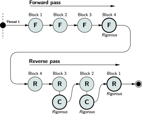
3.1.3. Second phase for intermediate blocks

For a network segmented into two blocks (A and B), a single forward pass adjustment and a single reverse pass adjustment are sufficient to achieve rigorous parameter estimates for Blocks B and A respectively. When a network is segmented into three or more blocks, the parameter estimates of all intermediate blocks estimated from both forward and reverse passes will be non-rigorous. This occurs because the intermediate blocks in both cases receive contribution from all preceding blocks only. To achieve rigorous parameter estimates for intermediate blocks, another second phase solution is required to combine the contribution of measurements and constraints contained in succeeding blocks.

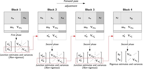
To illustrate how this is achieved, Figures 6 and 7 show the forward pass and reverse pass adjustments for a network segmented into four blocks.

6. Forward pass phased adjustment leading to rigorous estimates and variance matrix for Block 4 only.

7. Reverse pass phased adjustment leading to rigorous estimates and variance matrix for Block 1 only.

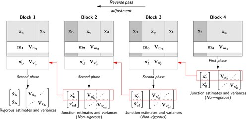
As Figure 6 indicates, the adjustment of Block 1 during the forward pass has been solved using a first phase adjustment (cf. Section 3.1.1). Blocks 2, 3 and 4 have been adjusted using a second phase adjustment (cf. Section 3.1.2). Similarly, for the reverse pass shown in Figure 7, Block 4 has been adjusted using a first phase adjustment and Blocks 3, 2 and 1 using second phase adjustment. The estimates and variances for Block 4 produced from the forward pass adjustment, and the estimates and variances for Block 1 produced from the reverse pass adjustment are rigorous as they are based on the contribution from all measurements in the network.

Figure 8 shows a second phase solution for Block 3, which must be completed for all intermediate blocks as part of a combination adjustment. In this solution, the contribution from Blocks 1 and 2 represented by ${\mathbf{x}}_{\mathbf{d}}^{\prime }$ and ${\mathbf{V}}_{{\mathbf{x}}_{\mathbf{d}}^{\prime }}$ (generated during the forward pass), and the contribution from Block 4 represented by ${\mathbf{x}}_{\mathbf{f}}^{\prime }$ and ${\mathbf{V}}_{{\mathbf{x}}_{\mathbf{f}}^{\prime }}$ (generated during the reverse pass), are combined with the measurements and precisions of Block 3. Similarly, this combination solution must also be undertaken for Block 2, which combines the measurements and precisions of Block 2, the (forward pass) junction parameter estimates and variances for Block 1, and the (reverse pass) junction parameter estimates and variances in Block 3.

8. Combination pass phased adjustment leading to rigorous estimates and variance matrix for Block 3.

Alternatively, the rigorous estimates for Block 3 may be solved by combining forward pass estimates $[{\mathbf{x}}_{\mathbf{d}}^{\prime }{\mathbf{x}}_{\mathbf{e}}^{\prime }{\mathbf{x}}_{\mathbf{f}}^{\prime }{]}^T$ with reverse pass estimates $[{\mathbf{x}}_{\mathbf{d}}^{″}{\mathbf{x}}_{\mathbf{e}}^{″}{\mathbf{x}}_{\mathbf{f}}^{″}{]}^T$. In this case, the observation equations are simply: (24) $\left[\begin{array}{c}{\mathbf{x}}_{\mathbf{d}}^{\prime }\\ {\mathbf{x}}_{\mathbf{e}}^{\prime }\\ {\mathbf{x}}_{\mathbf{f}}^{\prime }\\ {\mathbf{x}}_{\mathbf{d}}^{″}\\ {\mathbf{x}}_{\mathbf{e}}^{″}\\ {\mathbf{x}}_{\mathbf{f}}^{″}\end{array}\right]=\left[\begin{array}{ccc}\mathbf{I}& \mathbf{0}& \mathbf{0}\\ \mathbf{0}& \mathbf{I}& \mathbf{0}\\ \mathbf{0}& \mathbf{0}& \mathbf{I}\\ \mathbf{I}& \mathbf{0}& \mathbf{0}\\ \mathbf{0}& \mathbf{I}& \mathbf{0}\\ \mathbf{0}& \mathbf{0}& \mathbf{I}\end{array}\right]\left[\begin{array}{c}{\mathbf{x}}_{\mathbf{d}}\\ {\mathbf{x}}_{\mathbf{e}}\\ {\mathbf{x}}_{\mathbf{f}}\end{array}\right],\mathrm{w}\mathrm{i}\mathrm{t}\mathrm{h}{\mathbf{V}}_{{\mathbf{x}}_{\mathbf{d}\mathbf{e}\mathbf{f}}^{\prime }},{\mathbf{V}}_{{\mathbf{x}}_{\mathbf{d}\mathbf{e}\mathbf{f}}^{″}},$(24) where ${\mathbf{V}}_{{\mathbf{x}}_{\mathbf{d}\mathbf{e}\mathbf{f}}^{\prime }}$ and ${\mathbf{V}}_{{\mathbf{x}}_{\mathbf{d}\mathbf{e}\mathbf{f}}^{″}}$ are the full variance matrices produced from the forward and reverse pass solutions of Block 3, being: (25) ${\mathbf{V}}_{{\mathbf{x}}_{\mathbf{d}\mathbf{e}\mathbf{f}}^{\prime }}=\left[\begin{array}{ccc}{\mathbf{V}}_{{\mathbf{x}}_{\mathbf{d}}^{\prime }}& & \text{.}\text{.}\text{.}\\ & {\mathbf{V}}_{{\mathbf{x}}_{\mathbf{e}}^{\prime }}& \\ \text{.}\text{.}\text{.}& & {\mathbf{V}}_{{\mathbf{x}}_{\mathbf{f}}^{\prime }}\end{array}\right],{\mathbf{V}}_{{\mathbf{x}}_{\mathbf{d}\mathbf{e}\mathbf{f}}^{″}}=\left[\begin{array}{ccc}{\mathbf{V}}_{{\mathbf{x}}_{\mathbf{d}}^{″}}& & \text{.}\text{.}\text{.}\\ & {\mathbf{V}}_{{\mathbf{x}}_{\mathbf{e}}^{″}}& \\ \text{.}\text{.}\text{.}& & {\mathbf{V}}_{{\mathbf{x}}_{\mathbf{f}}^{″}}\end{array}\right].$(25) When forward, reverse and combination passes are complete, all estimates are rigorous due to the fact that the contribution from all measurements, measurement variances and parameter constraints from the entire network have been carried through successive blocks via the junction estimates and variances.

3.2. Simultaneous least squares solution

Here, the solution of estimates for $[{\hat{\mathbf{x}}}_{\mathbf{q}}{\hat{\mathbf{x}}}_{\mathbf{r}}{]}^T$ in Equation (23(23) $\begin{array}{rl}\left[\begin{array}{c}{\hat{\mathbf{x}}}_{\mathbf{q}}\\ {\hat{\mathbf{x}}}_{\mathbf{r}}\end{array}\right]& ={\left[\begin{array}{cc}{\mathbf{C}}_{22}-{\mathbf{C}}_{21}{\mathbf{C}}_{11}^{-1}{\mathbf{C}}_{12}+{\mathbf{D}}_{11}& {\mathbf{D}}_{12}\\ {\mathbf{D}}_{21}& {\mathbf{D}}_{22}\end{array}\right]}^{-1}\\ & \times \left[\begin{array}{cc}-{\mathbf{C}}_{21}{\mathbf{C}}_{11}^{-1}{\mathbf{C}}_1+{\mathbf{C}}_2& {\mathbf{D}}_1\\ \mathbf{0}& {\mathbf{D}}_2\end{array}\right]\left[\begin{array}{c}{\mathbf{m}}_{\mathbf{a}}\\ {\mathbf{m}}_{\mathbf{b}}\end{array}\right].\end{array}$(23) ) from a phased adjustment is proven to be identical to that produced from a partial solution and therefore rigorous. With reference to the segmented network in Figure 1 and distribution of parameters and measurements in Table 1, Figure 9 illustrates a simultaneous solution.

9. Simultaneous solution of a segmented network.

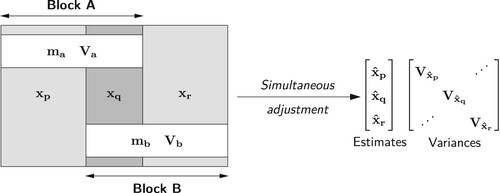
The simultaneous solution of the network shown in Figure 9 has observation equations in the form of Equation (1(1) $\left[\begin{array}{c}{\mathbf{m}}_{\mathbf{a}}\\ {\mathbf{m}}_{\mathbf{b}}\end{array}\right]=\left[\begin{array}{ccc}{\mathbf{A}}_1& {\mathbf{A}}_2& \mathbf{0}\\ \mathbf{0}& {\mathbf{B}}_1& {\mathbf{B}}_2\end{array}\right]\left[\begin{array}{c}{\mathbf{x}}_{\mathbf{p}}\\ {\mathbf{x}}_{\mathbf{q}}\\ {\mathbf{x}}_{\mathbf{r}}\end{array}\right],{\mathbf{V}}_{\mathbf{m}}=\left[\begin{array}{cc}{\mathbf{V}}_{\mathbf{a}}& \mathbf{0}\\ \mathbf{0}& {\mathbf{V}}_{\mathbf{b}}\end{array}\right]$(1) ), repeated here as (26) $\left[\begin{array}{c}{\mathbf{m}}_{\mathbf{a}}\\ {\mathbf{m}}_{\mathbf{b}}\end{array}\right]=\left[\begin{array}{ccc}{\mathbf{A}}_1& {\mathbf{A}}_2& \mathbf{0}\\ \mathbf{0}& {\mathbf{B}}_1& {\mathbf{B}}_2\end{array}\right]\left[\begin{array}{c}{\mathbf{x}}_{\mathbf{p}}\\ {\mathbf{x}}_{\mathbf{q}}\\ {\mathbf{x}}_{\mathbf{r}}\end{array}\right],{\mathbf{V}}_{\mathbf{m}}=\left[\begin{array}{cc}{\mathbf{V}}_{\mathbf{a}}& \mathbf{0}\\ \mathbf{0}& {\mathbf{V}}_{\mathbf{b}}\end{array}\right].$(26) Here, matrices ${\mathbf{A}}_1$ and ${\mathbf{A}}_2$ represent the design matrix elements associated with the parameters ${\mathbf{x}}_{\mathbf{p}}$ and ${\mathbf{x}}_{\mathbf{q}}$ in Block A. ${\mathbf{B}}_1$ and ${\mathbf{B}}_2$ represent the design matrix elements associated with the parameters ${\mathbf{x}}_{\mathbf{q}}$ and ${\mathbf{x}}_{\mathbf{r}}$ in Block B. It is assumed that the parameters have been ordered so that they can be neatly partitioned as shown in Equation (26(26) $\left[\begin{array}{c}{\mathbf{m}}_{\mathbf{a}}\\ {\mathbf{m}}_{\mathbf{b}}\end{array}\right]=\left[\begin{array}{ccc}{\mathbf{A}}_1& {\mathbf{A}}_2& \mathbf{0}\\ \mathbf{0}& {\mathbf{B}}_1& {\mathbf{B}}_2\end{array}\right]\left[\begin{array}{c}{\mathbf{x}}_{\mathbf{p}}\\ {\mathbf{x}}_{\mathbf{q}}\\ {\mathbf{x}}_{\mathbf{r}}\end{array}\right],{\mathbf{V}}_{\mathbf{m}}=\left[\begin{array}{cc}{\mathbf{V}}_{\mathbf{a}}& \mathbf{0}\\ \mathbf{0}& {\mathbf{V}}_{\mathbf{b}}\end{array}\right].$(26) ).

While the ordering is not critical for a simultaneous solution, the segmentation algorithm (discussed in Section 4) automatically organises the system of equations according to the parameters to which they relate and then subdivides all equations into blocks based upon the selection of parameters for each block. The segmentation algorithm also identifies measurements which are correlated (such as GNSS position and baseline clusters) and ensures they are grouped within blocks accordingly.

Taking abbreviations from Equations (15(15) $\begin{array}{cc}{\mathbf{C}}_{ij}& ={\mathbf{A}}_i^T{\mathbf{V}}_{\mathbf{a}}^{-1}{\mathbf{A}}_j,\mathrm{w}\mathrm{i}\mathrm{t}\mathrm{h}i=1\dots 2;j=1\dots 2\\ {\mathbf{C}}_i& ={\mathbf{A}}_i^T{\mathbf{V}}_{\mathbf{a}}^{-1},\mathrm{w}\mathrm{i}\mathrm{t}\mathrm{h}i=1\dots 2.\end{array}$(15) ) and (22(22) $\begin{array}{rl}{\mathbf{D}}_{ij}& ={\mathbf{B}}_i^T{\mathbf{V}}_{\mathbf{b}}^{-1}{\mathbf{B}}_j,\mathrm{w}\mathrm{i}\mathrm{t}\mathrm{h}i=1\dots 2;j=1\dots 2\\ {\mathbf{D}}_i& ={\mathbf{B}}_i^T{\mathbf{V}}_{\mathbf{b}}^{-1},\mathrm{w}\mathrm{i}\mathrm{t}\mathrm{h}i=1\dots 2.\end{array}$(22) ), the simultaneous least squares solution of Equation (26(26) $\left[\begin{array}{c}{\mathbf{m}}_{\mathbf{a}}\\ {\mathbf{m}}_{\mathbf{b}}\end{array}\right]=\left[\begin{array}{ccc}{\mathbf{A}}_1& {\mathbf{A}}_2& \mathbf{0}\\ \mathbf{0}& {\mathbf{B}}_1& {\mathbf{B}}_2\end{array}\right]\left[\begin{array}{c}{\mathbf{x}}_{\mathbf{p}}\\ {\mathbf{x}}_{\mathbf{q}}\\ {\mathbf{x}}_{\mathbf{r}}\end{array}\right],{\mathbf{V}}_{\mathbf{m}}=\left[\begin{array}{cc}{\mathbf{V}}_{\mathbf{a}}& \mathbf{0}\\ \mathbf{0}& {\mathbf{V}}_{\mathbf{b}}\end{array}\right].$(26) ) can be simplified as (27) $\left[\begin{array}{c}{\hat{\mathbf{x}}}_{\mathbf{p}}\\ ---\\ {\hat{\mathbf{x}}}_{\mathbf{q}}\\ {\hat{\mathbf{x}}}_{\mathbf{r}}\end{array}\right]={\left[\begin{array}{ccc}{\mathbf{C}}_{11}& {\mathbf{C}}_{12}& \mathbf{0}\\ {\mathbf{C}}_{21}& {\mathbf{C}}_{22}+{\mathbf{D}}_{11}& {\mathbf{D}}_{12}\\ \mathbf{0}& {\mathbf{D}}_{21}& {\mathbf{D}}_{22}\end{array}\right]}^{-1}\left[\begin{array}{c}{\mathbf{C}}_1\mathbf{0}\\ ----\\ {\mathbf{C}}_2{\mathbf{D}}_1\\ \mathbf{0}{\mathbf{D}}_2\end{array}\right]\left[\begin{array}{c}{\mathbf{m}}_{\mathbf{a}}\\ {\mathbf{m}}_{\mathbf{b}}\end{array}\right].$(27) Using Equation (A13(A13) ${\mathbf{x}}_2=[-{[{\mathbf{E}}_{22}-{\mathbf{E}}_{21}{\mathbf{E}}_{11}^{-1}{\mathbf{E}}_{12}]}^{-1}]\left[\begin{array}{cc}{\mathbf{E}}_{21}{\mathbf{E}}_{11}^{-1}& \mathbf{I}\end{array}\right]\left[\begin{array}{c}{\mathbf{y}}_1\\ {\mathbf{y}}_2\end{array}\right].$(A13) ) in Appendix, the partial solution of parameter estimates ${\hat{\mathbf{x}}}_{\mathbf{q}}$ and ${\hat{\mathbf{x}}}_{\mathbf{r}}$ from the total solution can be solved as (28) $\begin{array}{rl}\left[\begin{array}{cc}{\hat{\mathbf{x}}}_{\mathbf{q}}& \\ {\hat{\mathbf{x}}}_{\mathbf{r}}\end{array}\right]& ={[\left[\begin{array}{cc}{\mathbf{C}}_{22}+{\mathbf{D}}_{11}& {\mathbf{D}}_{12}\\ {\mathbf{D}}_{21}& {\mathbf{D}}_{22}\end{array}\right]-\left[\begin{array}{c}{\mathbf{C}}_{21}\\ \mathbf{0}\end{array}\right]{\mathbf{C}}_{11}^{-1}\left[\begin{array}{cc}{\mathbf{C}}_{12}& \mathbf{0}\end{array}\right]]}^{-1}\\ & \times [-\begin{array}{cc}\left[\begin{array}{c}{\mathbf{C}}_{21}\\ \mathbf{0}\end{array}\right]{\mathbf{C}}_{11}^{-1}& \left[\begin{array}{cc}\mathbf{I}& \mathbf{0}\\ \mathbf{0}& \mathbf{I}\end{array}\right]\end{array}]\left[\begin{array}{c}{\mathbf{C}}_1\mathbf{0}\\ ----\\ {\mathbf{C}}_2{\mathbf{D}}_1\\ \mathbf{0}{\mathbf{D}}_2\end{array}\right]\left[\begin{array}{c}{\mathbf{m}}_{\mathbf{a}}\\ {\mathbf{m}}_{\mathbf{b}}\end{array}\right].\end{array}$(28) After simplification, the partial solution for parameter estimates ${\hat{\mathbf{x}}}_{\mathbf{q}}$ and ${\hat{\mathbf{x}}}_{\mathbf{r}}$ can be expressed as (29) $\begin{array}{rl}\left[\begin{array}{c}{\hat{\mathbf{x}}}_{\mathbf{q}}\\ {\hat{\mathbf{x}}}_{\mathbf{r}}\end{array}\right]& ={\left[\begin{array}{cc}{\mathbf{C}}_{22}-{\mathbf{C}}_{21}{\mathbf{C}}_{11}^{-1}{\mathbf{C}}_{12}+{\mathbf{D}}_{11}& {\mathbf{D}}_{12}\\ {\mathbf{D}}_{21}& {\mathbf{D}}_{22}\end{array}\right]}^{-1}\\ & \times \left[\begin{array}{cc}-{\mathbf{C}}_{21}{\mathbf{C}}_{11}^{-1}{\mathbf{C}}_1+{\mathbf{C}}_2& {\mathbf{D}}_1\\ \mathbf{0}& {\mathbf{D}}_2\end{array}\right]\left[\begin{array}{c}{\mathbf{m}}_{\mathbf{a}}\\ {\mathbf{m}}_{\mathbf{b}}\end{array}\right].\end{array}$(29)

Note that the partial estimates for $[{\hat{\mathbf{x}}}_{\mathbf{q}}{\hat{\mathbf{x}}}_{\mathbf{r}}{]}^T$ in Equation (29(29) $\begin{array}{rl}\left[\begin{array}{c}{\hat{\mathbf{x}}}_{\mathbf{q}}\\ {\hat{\mathbf{x}}}_{\mathbf{r}}\end{array}\right]& ={\left[\begin{array}{cc}{\mathbf{C}}_{22}-{\mathbf{C}}_{21}{\mathbf{C}}_{11}^{-1}{\mathbf{C}}_{12}+{\mathbf{D}}_{11}& {\mathbf{D}}_{12}\\ {\mathbf{D}}_{21}& {\mathbf{D}}_{22}\end{array}\right]}^{-1}\\ & \times \left[\begin{array}{cc}-{\mathbf{C}}_{21}{\mathbf{C}}_{11}^{-1}{\mathbf{C}}_1+{\mathbf{C}}_2& {\mathbf{D}}_1\\ \mathbf{0}& {\mathbf{D}}_2\end{array}\right]\left[\begin{array}{c}{\mathbf{m}}_{\mathbf{a}}\\ {\mathbf{m}}_{\mathbf{b}}\end{array}\right].\end{array}$(29) ) are identical to the estimates obtained from the second phase solution expressed in Equation (23(23) $\begin{array}{rl}\left[\begin{array}{c}{\hat{\mathbf{x}}}_{\mathbf{q}}\\ {\hat{\mathbf{x}}}_{\mathbf{r}}\end{array}\right]& ={\left[\begin{array}{cc}{\mathbf{C}}_{22}-{\mathbf{C}}_{21}{\mathbf{C}}_{11}^{-1}{\mathbf{C}}_{12}+{\mathbf{D}}_{11}& {\mathbf{D}}_{12}\\ {\mathbf{D}}_{21}& {\mathbf{D}}_{22}\end{array}\right]}^{-1}\\ & \times \left[\begin{array}{cc}-{\mathbf{C}}_{21}{\mathbf{C}}_{11}^{-1}{\mathbf{C}}_1+{\mathbf{C}}_2& {\mathbf{D}}_1\\ \mathbf{0}& {\mathbf{D}}_2\end{array}\right]\left[\begin{array}{c}{\mathbf{m}}_{\mathbf{a}}\\ {\mathbf{m}}_{\mathbf{b}}\end{array}\right].\end{array}$(23) ), demonstrating the rigour of Tienstra's principle of least squares adjustment in phases.

4. Automatic network segmentation

In this section, we review the prerequisite features of subdividing a network to achieve a rigorous solution from Tienstra's method of phased adjustment. We then present the automatic segmentation algorithm and explain how it provides a highly efficient, flexible and scalable approach to the task of re-subdividing extremely large networks subject to continual change. The first point to note from this section is that the segmentation algorithm does not rely upon subdivision by geographical area and nested hierarchies, but rather, measurement connectivity. The second point is that a block can be comprised of parameters located in remote areas of the network not connected by direct measurement. The third point to note is that segmentation can be configured so that the parameters and full variance matrix can be estimated for a selection of specific stations whether they are connected by measurement or not.

4.1. Principles of segmentation for Tienstra's method

When solving for parameters via Tienstra's method, the number of ways a system of measurements may be divided is almost endless, provided certain conditions are satisfied. Conceptually, a network can be partitioned into any number of blocks.

According to Tienstra's method, junction parameters and their variances are carried between blocks as pseudo measurements (or cofactors in the language of Tienstra) and may appear in several other blocks. When a junction parameter is no longer required to be carried to other blocks, it appears as an inner parameter.

There is no limit on the way a measurement set can be segmented, apart from a consideration of (i) measurement connectivity; (ii) correlated measurements; (iii) number of parameters to which block sizes are to be limited and (iv) which parameters should be included in the first block (see Section 4.2). Therefore, the only prerequisite features of subdividing a network for solution by Tienstra's method are:

• Inner parameter stations within a block must have all measurements connected to them within that block. That is, an inner parameter must not be connected to a parameter in another block by measurement. In addition, an inner station must only appear in a single block.

• All junction parameter stations must be associated with one or more measurements in two or more blocks. A junction station may appear in zero or multiple blocks. When all measurements connected to a junction parameter are exhausted, that parameter becomes an inner.

These being the only prerequisites, tremendous flexibility in the way a network can be subdivided is granted. So also is a fresh opportunity to achieve a high level of automation.

4.2. Automatic segmentation algorithm

A fully-automated segmentation algorithm that preserves Tienstra's principle of phased least squares (Tienstra 1956) has been developed. The algorithm is based on the work of Leahy (1999) and Leahy and Collier (1998) and caters for a vast array of correlated and non-correlated GNSS and terrestrial measurements. The algorithm subdivides a system of linear parameterised equations using concepts drawn from graph theory (Cormen 2001), by which univariate or multivariate parameters (e.g. height, horizontal location or 3D position) are treated as nodes (i.e. parameter stations). A node may be connected by one or more correlated or non-correlated measurements. Owing to the linear connectivity between parameter stations and measurements, the algorithm is adaptive, configurable and offers an unprecedented level of efficiency and flexibility over former blocking methods.

The behaviour of the formation of each block is a function of the following:

• Measurement connectivity. The algorithm forms blocks sequentially according to the station and measurement connectivity found in the system of linearised observation equations, and capably responds to any level of connectivity and any combination of measurement types. The algorithm is optimised to deal with isolated measurement sets, user-specified block sizes, and to automatically select new stations according to the number of measurements connected to each station. This yields optimal levels of performance by preventing excessively large blocks from being formed.

• Stochastic correlation. Measurements which are stochastically correlated are tightly coupled and introduce correlated stations as a single cluster. Thus GNSS baseline clusters and correlated GNSS station position with a full variance matrix, and sets (or rounds) of correlated horizontal directions are not subdivided across multiple blocks. This ensures all parameters and their variances are solved and passed between blocks in a rigorous way.

• Block size limit. A (user-supplied) restriction may be placed upon on the number of parameters each block should contain. This argument restricts the normal matrix for each block to a size matched to available computational resources and amount of parallelism that can be achieved. When attempting to solve large numbers of parameters from extremely large measurement sets, being able to set a block size limit is essential for achieving the optimal level of performance based on CPU clock speed and multi-core architecture.

• Block-1 parameters. Since the algorithm sequentially assembles each block according to station-to-measurement connectivity, it is possible for two or more stations of particular interest to appear in different blocks. For this reason, a (user-supplied) list of stations can be nominated for inclusion in the first block. Optional selection of Block-1 stations permits:

  	(1)	The full variance matrix of parameters of interest to be derived efficiently without further computation or necessity to store the covariances between all parameters.
  	(2)	Minimised processing time to rigorously estimate selected parameters and variances from the entire set by not having to compute parameters and variances for all other blocks in the network, which reduces the computation time, by at least 50%.
  	(3)	Rigorous computation of relative precisions between any two or more stations between which there are no direct measurements.

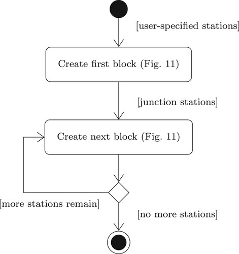
The automatic segmentation procedure involves the creation of the first block, commencing with a user-specified set of stations (or the first station in an ordered list if no stations have been specified), and then the sequential creation of all other blocks. The high-level procedure is shown in Figure 10. The procedure for forming individual blocks is shown in Figure 11. At the end of the high-level procedure shown in Figure 10, each block will contain three lists – a list of ${\mathbf{i}}_{1\dots i}$ inner stations, a list of ${\mathbf{j}}_{0\dots j}$ junction stations and a list of ${\mathbf{m}}_{1\dots m}$ measurements.

10. High-level automatic segmentation procedure.

11. Automatic segmentation procedure for creating individual blocks.

With reference to Figure 11, the sequence of steps is explained as follows.

(1)	Starting station(s) or junction(s) from the previous block. On entry, the list of stations will contain $0\dots n$ user-supplied stations for the first block (or the first freely available station in an ordered list if no stations have been specified), or $0\dots j$ junction stations passed forward from the previous block.
(2)	Add new junction from inners. If the network contains isolated (non-contiguous) networks, the junctions for this block (i.e. the first block in the next isolated network) will be empty. In this case, the next freely available station is introduced as a junction.
(3)	Set junction as an inner. The next available junction (from step 1 or 2) is added to the list of inner stations.
(4)	Get connected measurements. All measurements connected to this station are added to the block. During this process, any stations connected to the recently added measurements that are not already in the list of junctions and inners are introduced as a junction. At this point, a test is performed to determine if the block size threshold has been exceeded. If the aggregate number of stations in the inner and junction lists exceeds the block size threshold, the block formation procedure works towards completing the block (step 5 onward). Otherwise, the algorithm repeats steps 1, 2, 3 and 4. If no further stations are available for consideration, the algorithm proceeds to step 5.
(5)	Find common measurements. When no more junctions can be moved to the list of inners, the algorithm adds to the block all measurements which are wholly connected to the inner stations.
(6)	Set junction as an inner. Any stations in the list of junctions that have all the measurements connected to them already in the block, are then moved to the list of inners. The structure of the block is now complete and is made up of inner stations, junction stations and connected measurements.

5. Parallel phased least squares estimation

Theoretically, the phased least squares technique allows for the rigorous estimation of any number of parameters and measurements, whether in the order of tens or millions. While variation in the number and composition of blocks may have an impact on the computational processing time, they will not affect the rigour of the solution. Strictly speaking, the only real limitations are those which are imposed by a computer's processor, physical memory and operating system memory model.

Motivated by an opportunity to take full advantage of modern multi-core architectures, we have developed a scalable phased least squares parallelisation strategy based on a dynamic multi-threaded scheduling scheme. The objectives of the strategy are to parallelise the non-sequential tasks of Tienstra's phased least squares method so as to maximise the full potential of multi-core processors.

To illustrate the concept, consider the processing of forward, reverse and combination passes in a single process shown by Figure 12. In single-thread mode, all least squares operations are executed in a sequential fashion on one thread managed by a single core.

12. Sequential execution of forward (F), reverse (R) and combination (C) passes on a single core.

Although outstanding performance can be realised in sequential mode by using parallel factorisation libraries, such as Scalable Linear Algebra PACKage (ScaLAPACK) (Choi et al. 1996), Math Kernel Library (MKL) (Intel 2020) and Parallel Linear Algebra for Scalable Multi-core Architectures (PLASMA) (Buttari et al. 2009; Dongarra et al. 2019), improved levels of performance with full CPU utilisation can be achieved (discussed in Section 6) by parallelising forward, reverse and combination passes. Parallelisation of these passes is illustrated in Figure 13.

13. Parallel execution of forward (F), reverse (R) and combination (C) pass adjustments on multiple cores.

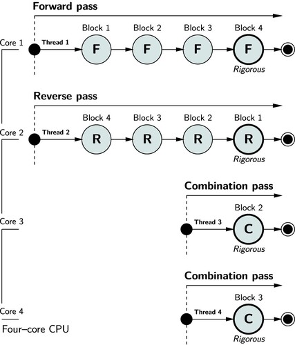
At the time of execution, both forward and reverse passes are executed concurrently on two cores. Synchronisation between concurrent forward and reverse threads is undertaken to monitor the completion of blocks and to ensure the essential sequencing requirements of Tienstra's method. When an intermediate block has been solved by both forward (c.f. Figure 6) and reverse (c.f. Figure 7) passes, that block is added to a queue that asynchronously schedules execution of combination (c.f. Figure 8) adjustments on unique threads.

If a computer has at least four cores, all threads can be executed in parallel which will achieve the fastest estimation time. Hence, running phased least squares in multi-thread mode on a quad core CPU will result in 100% utilisation of the computer's processing capability. With CPUs having 8 cores and hyper-threading technology, unprecedented performance gains can be achieved with this strategy, especially when coupled with a parallel factorisation library. These developments yield a highly efficient parallel phased least squares approach that is scalable and responsive to processor clock speeds and memory capacity.

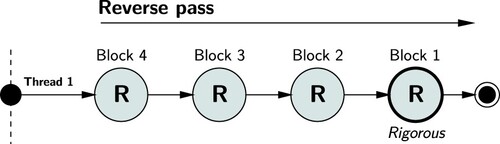
If only the parameter estimates and full variance matrix for the first block is required, a reverse pass solution can be executed alone. This alleviates the need to execute forward pass and combination pass adjustments, meaning that the time to solve the first block can be reduced to almost a third of the total time to undertake a sequential solution (c.f. Figure 12). The reverse pass only concept is shown in Figure 14.

14. Execution of reverse (R) pass only adjustment.

6. Case study – routine maintenance of Australia's national reference frame

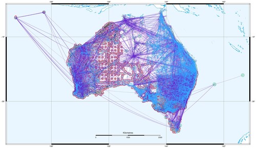
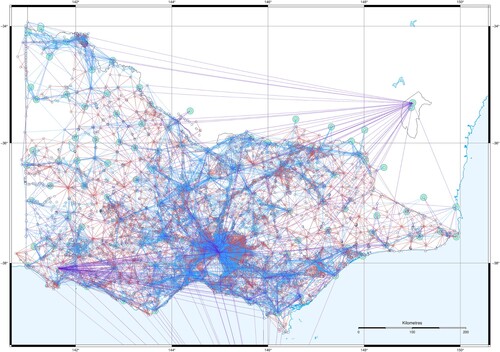
In this section, we review the application of these developments to the routine maintenance of Australia's national reference frame from an extremely large and continually evolving measurement set. Figure 15 shows the national geodetic network used for the establishment and routine maintenance of Australia's national reference frame, known as the Geocentric Datum of Australia 2020 (GDA2020). Figure 16 shows the Victorian component – one of eight (federated) jurisdictional sub-networks making up the national network.

15. Australia's national geodetic network, comprising 762,273 parameters and 1,897,242 GNSS and terrestrial measurements.

16. Victoria's state geodetic network, comprising 132,936 parameters and 284,900 GNSS and terrestrial measurements.

Using an open-source software package that implements the developments described in this paper, these large networks can be routinely segmented and solved in a fraction of the time required by traditional blocking and adjustment strategies.

The Victorian geodetic network shown in Figure 16 is comprised of 132,936 (3D) coordinate parameters and 284,900 GNSS, distance, direction, vertical angle and height measurements. Each week, new GNSS measurements are processed and added to this network, which in turn is solved to produce new parameter estimates. The same procedure is followed in each other jurisdiction.

Using an affordable desktop computer (e.g. Intel i7 9700 CPU @ 3.00GHz, with 8 cores allowing 8 concurrent threads of execution), full segmentation of the entire network takes 1.8 seconds and results in 73 blocks. Solution of all parameters takes 1 minute 50 seconds per iteration. Upon the introduction of new measurements, new 3D coordinates and rigorous variances can be generated and made available to external stakeholders almost instantaneously. With a capacity to perform a reverse (Block-1 only) solution (c.f. Figures 7 and 14), rigorous parameters and full variance matrix for a list of user-specified stations can be generated (including full re-segmentation) in less than 1 minute.

At the time of writing, Australia's national geodetic network shown in Figure 15 is comprised of 762,273 parameters connected to 1,897,242 GNSS measurements and terrestrial measurements. Table 2 summarises the GNSS and terrestrial measurement types contained in this dataset.

Table 2. Summary of measurements comprising Australia's national geodetic network.

Measurement type	Count
GPS baseline	1,107,762
GPS baseline cluster	68,820
GPS point cluster	1,902
Geodetic azimuth	1,536
Horizontal direction sets	326,702
Astronomic azimuth	132
Zenith angle	203
Level difference	4,931
Orthometric height	130,955
Ellipsoid arc	7,663
Mean sea level arc	200,258
Slope distance	46,378
Total	1,897,242

The GNSS point clusters represent solutions with full variance matrices from episodic GNSS campaigns and GNSS Continuously Operating Reference Station (CORS) sites located on mainland Australia and its associated islands. Similarly, each GNSS baseline cluster is a fully correlated measurement set with full variance matrix.

By selecting empirically derived segmentation parameters that achieves optimal performance, this network is segmented into 80 blocks, ranging in size from 8 to 22,329 parameters. Segmentation of this network takes, on average, around 45 seconds. The solution of all 762,273 parameters including rigorous variance matrices for all 80 blocks is undertaken on Australia's National Computational Infrastructure (NCI) Gadi supercomputer. Gadi is Australia's most powerful supercomputer and is ranked 57 on the TOP500 supercomputer list (TOP500 2022). The specific node on which this solution is executed has 32 CPU cores (2 nodes each with 2 sockets and 8 cores/socket), has access to 4TB physical memory and is managed by CentOS 6.4 (Linux).

Using parallel phased least squares, the solution of all parameter estimates and full variance matrix for each block takes approximately 1 hour 38 minutes per iteration and consumes almost 2.82 TB of memory. Using sequential phased least squares, each iteration takes approximately 2 hours 3 minutes per iteration and consumes approximately 1.4 TB of memory. With ongoing GNSS measurement and regeneration of jurisdictional sub-network solutions managed by six states and two territories, re-segmentation and re-estimation of GDA2020 is performed every month using an entirely automated process.

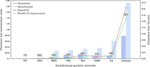
Figure 17 shows the average increase in performance (%) that is typically realised when using the parallel strategy over the time taken to perform the same solution using the sequential strategy for each jurisdictional network and the entire national network. For this graph, the estimation times for all jurisdictional geodetic networks were generated on a consumer-level desktop computer. The estimation times for the national network were generated on Gadi. The reason for the lower performance improvement on Gadi is largely attributable to its massively parallel CPU architecture being distributed over a number of nodes and hence, the trade off in distributing information among the CPU nodes.

17. Performance improvement of parallel phased least squares over sequential phased least squares estimation time.

The reason parallel phased least squares requires over twice the amount of memory is due to the need to manipulate separate copies of the least squares matrices (e.g. normals, weighted measurements and coefficients, junction parameter estimates and variances) for forward and reverse passes. If large physical memory capacity is unavailable, the software can be set to use memory-mapped files on the hard disk to hold all the necessary least squares information. In this mode, phased least squares solutions of the national network take approximately 2 hours 40 minutes per iteration and require less than 4 GB of memory (i.e. the largest amount of memory required to process one block at a time).

In any case, with the availability of on-demand, scalable cloud computing infrastructure, virtual servers with the desired level of capacity (up to 24 TB of memory) can be marshalled to perform the full solutions as and when required, without the need to purchase and maintain highly expensive computer hardware. This affords a unique opportunity to deliver high levels of dynamism in reference frame maintenance.

7. Conclusion and further work

This paper has presented a novel automatic segmentation algorithm and parallel phased least squares strategy, which provide significant advancements in geodetic methodology concerning the performance of solving massive and constantly changing systems. The ability to automatically segment a large set of parameters and measurements into manageable sized blocks, according to user preference, offers considerable versatility and scalability. These developments offer a breakthrough in geodetic methodology, in that for the first time they allow for the rigorous solution of both parameters and variances from massive systems of observation equations subject to continual change in an adaptive and highly efficient manner. The benefits of these developments are summarised as follows.

First, they permit the user to fine tune the segmentation parameters to achieve optimal results according to CPU. Second, they enable the rigorous estimation of parameter estimates and precisions for any two or more parameters irrespective of the absence of direct measurements between them or the way the network has been segmented. Third, having an ability to nominate which parameters should be contained within the first block, rigorous parameter estimates and their precisions for these parameters can be generated by a reverse pass adjustment alone without the having to undertake forward pass or combination adjustments, thereby reducing the time by a factor of two again. Fourth, they enable users to generate a variance matrix for the parameters in the first block almost instantly, removing the complexities involved in archiving and interrogating extremely large variance matrices. Fifth, with an automated segmentation procedure which permits the user to quickly and easily segment networks of almost any size, users can repeatedly estimate three-dimensional positions from extremely large systems of measurements subject to continual expansion and change.

With the incessant requirement to deliver up-to-date coordinates and uncertainties of geodetic networks and digital cadastre fabrics, traceable to global reference frames, these developments provide an unprecedented opportunity for the development and routine maintenance of dynamic datums based on massive and constantly changing datasets.

Finally, further investigation into increasing the level of adaptiveness, parallelism and computational performance is warranted. The optimal performance of the least squares solution relies heavily on the user to nominate the segmentation parameters for generating the most appropriate size of each block according CPU clock speed. Similarly, manual selection of which strategy to undertake for the phased least squares solution, whether sequential (single-thread) or parallel (multi-thread), is required given the increased dependency parallelism has upon physical memory capacity. Manual selection at the present time is based on empirical values which are known to achieve optimal performance. The fine tuning of segmentation parameters and adjustment strategy according to computational resources at hand can at times take several attempts before optimal performance is achieved. In some cases, introducing a new set of measurements can lead to the need for different parameters. Further work is being undertaken to dynamically optimise the parameters and adjustment strategy at the time of execution based on CPU cores, clock speeds, physical and GPU memory models, parallel factorisation libraries, number of parameters, number of measurements (both correlated and uncorrelated) and the parameter-to-measurement connectivity. Consideration is also being given to the application of novel approaches for executing parallelism over distributed memory architectures to improve adaptiveness and computational performance based on network characteristics.

Acknowledgments

The authors would like to gratefully acknowledge the former Department of Environment, Land, Water and Planning and Geoscience Australia for their support, provision of data and access to Australia's National Computational Infrastructure (NCI). We also gratefully acknowledge John Dawson from Geoscience Australia and Chris Rizos from the University of New South Wales (UNSW) for their helpful suggestions and constructive feedback on this manuscript.

Disclosure statement

The authors report there are no competing interests to declare.

Additional information

Notes on contributors

Roger W. Fraser

Dr. Roger W Fraser is Chief Geospatial Scientist at the Department of Transport and Planning. Roger has been involved in several state and national geodetic and cadastral infrastructure projects including GDA94, GDA2020, Standard for the Australian Survey Control Network (SP1), AuScope GNSS, GeodesyML, DynAdjust and Victoria's digital cadastre modernisation. Roger's interests include geodesy, least squares estimation, GNSS analysis, software development, data modelling and digital cadastre automation.

Frank J. Leahy

Dr. Frank J. Leahy interest in geodesy developed over the four decades spent in academia at the University of Melbourne, Australia. His teaching and research were concentrated on broader issues of spatial science. His research was focused on algorithms for the delineation of maritime boundaries and the adjustment of geodetic networks. His particular interest was in “phased network adjustment”, as proposed by Tienstra, which led to the development of a network segmentation algorithm that allows the efficient sequential adjustment of large networks.

Philip A. Collier

Dr Philip A. Collier interests lie primarily in the fields of geodesy, high precision GNSS, least squares estimation, least squares collocation, geodetic computation and the broader application of spatial and geodetic principles to complex problems. In a career spanning 35 years, he has worked in academia and the private sector as well as serving as Research Director of the Australia-New Zealand Cooperative Research Centre for Spatial Information. He is currently Principal Consultant with Collier Geodetic Solutions, where he is working on projects in Australia and internationally.

Appendix. The partitioned model

A.1. Inverse of partitioned symmetric matrices

Given a positive definite symmetric matrix of full rank $\mathbf{E}$, the inverse of its partitioned form can be written as (A1) ${\mathbf{E}}^{-1}=\left[\begin{array}{cc}{\mathbf{E}}_{11}& {\mathbf{E}}_{12}\\ {\mathbf{E}}_{21}& {\mathbf{E}}_{22}\end{array}\right],$(A1) where the elements of ${\mathbf{E}}^{-1}$ are (A2) ${\mathbf{E}}_{11}={[{\mathbf{E}}_{11}-{\mathbf{E}}_{12}{\mathbf{E}}_{22}^{-1}{\mathbf{E}}_{21}]}^{-1}$(A2) (A3) ${\mathbf{E}}_{22}={[{\mathbf{E}}_{22}-{\mathbf{E}}_{21}{\mathbf{E}}_{11}^{-1}{\mathbf{E}}_{12}]}^{-1}$(A3) (A4) ${\mathbf{E}}_{12}=-{\mathbf{E}}_{11}^{-1}{\mathbf{E}}_{12}{[{\mathbf{E}}_{22}-{\mathbf{E}}_{21}{\mathbf{E}}_{11}^{-1}{\mathbf{E}}_{12}]}^{-1}$(A4) (A5) ${\mathbf{E}}_{21}=-{\mathbf{E}}_{22}^{-1}{\mathbf{E}}_{21}{[{\mathbf{E}}_{11}-{\mathbf{E}}_{12}{\mathbf{E}}_{22}^{-1}{\mathbf{E}}_{21}]}^{-1}.$(A5) As the inverse of $\mathbf{E}$ and the partitioned matrices ${\mathbf{E}}_{11}$ and ${\mathbf{E}}_{22}$ are symmetric, an alternative form of the inverse can be written by transposing and interchanging the off-diagonal terms. Therefore, Equations (A4(A4) ${\mathbf{E}}_{12}=-{\mathbf{E}}_{11}^{-1}{\mathbf{E}}_{12}{[{\mathbf{E}}_{22}-{\mathbf{E}}_{21}{\mathbf{E}}_{11}^{-1}{\mathbf{E}}_{12}]}^{-1}$(A4) ) and (A5(A5) ${\mathbf{E}}_{21}=-{\mathbf{E}}_{22}^{-1}{\mathbf{E}}_{21}{[{\mathbf{E}}_{11}-{\mathbf{E}}_{12}{\mathbf{E}}_{22}^{-1}{\mathbf{E}}_{21}]}^{-1}.$(A5) ) can be expressed as (A6) ${\mathbf{E}}_{12}=-{[{\mathbf{E}}_{11}-{\mathbf{E}}_{12}{\mathbf{E}}_{22}^{-1}{\mathbf{E}}_{21}]}^{-1}{\mathbf{E}}_{12}{\mathbf{E}}_{22}^{-1}$(A6) (A7) ${\mathbf{E}}_{21}=-{[{\mathbf{E}}_{22}-{\mathbf{E}}_{21}{\mathbf{E}}_{11}^{-1}{\mathbf{E}}_{12}]}^{-1}{\mathbf{E}}_{21}{\mathbf{E}}_{11}^{-1}.$(A7) This allows us to write ${\mathbf{E}}^{-1}$ as (A8) $\begin{array}{rl}{\mathbf{E}}^{-1}& =\left[\begin{array}{cc}{\left[{\mathbf{E}}_{11}-{\mathbf{E}}_{12}{\mathbf{E}}_{22}^{-1}{\mathbf{E}}_{21}\right]}^{-1}& \mathbf{0}\\ \mathbf{0}& {\left[{\mathbf{E}}_{22}-{\mathbf{E}}_{21}{\mathbf{E}}_{11}^{-1}{\mathbf{E}}_{12}\right]}^{-1}\end{array}\right]\\ & \times \left[\begin{array}{cc}\mathbf{I}& -{\mathbf{E}}_{12}{\mathbf{E}}_{22}^{-1}\\ -{\mathbf{E}}_{21}{\mathbf{E}}_{11}^{-1}& \mathbf{I}\end{array}\right].\end{array}$(A8) In this form, the partial solution of a set of simultaneous equations can be developed.

A.2. Solution of parameters from a partitioned model

For the set of observation equations: (A9) $\left[\begin{array}{c}{\mathbf{y}}_1\\ {\mathbf{y}}_2\end{array}\right]=\mathbf{E}\left[\begin{array}{c}{\mathbf{x}}_1\\ {\mathbf{x}}_2\end{array}\right]$(A9) the simultaneous solution of parameters ${\mathbf{x}}_{\mathbf{1}}$ and ${\mathbf{x}}_{\mathbf{2}}$ can be expressed as (A10) $\left[\begin{array}{c}{\mathbf{x}}_1\\ {\mathbf{x}}_2\end{array}\right]={\left[\begin{array}{cc}{\mathbf{E}}_{11}& {\mathbf{E}}_{12}\\ {\mathbf{E}}_{21}& {\mathbf{E}}_{22}\end{array}\right]}^{-1}\left[\begin{array}{c}{\mathbf{y}}_1\\ {\mathbf{y}}_2\end{array}\right].$(A10) Substituting Equation (A8(A8) $\begin{array}{rl}{\mathbf{E}}^{-1}& =\left[\begin{array}{cc}{\left[{\mathbf{E}}_{11}-{\mathbf{E}}_{12}{\mathbf{E}}_{22}^{-1}{\mathbf{E}}_{21}\right]}^{-1}& \mathbf{0}\\ \mathbf{0}& {\left[{\mathbf{E}}_{22}-{\mathbf{E}}_{21}{\mathbf{E}}_{11}^{-1}{\mathbf{E}}_{12}\right]}^{-1}\end{array}\right]\\ & \times \left[\begin{array}{cc}\mathbf{I}& -{\mathbf{E}}_{12}{\mathbf{E}}_{22}^{-1}\\ -{\mathbf{E}}_{21}{\mathbf{E}}_{11}^{-1}& \mathbf{I}\end{array}\right].\end{array}$(A8) ) for ${\mathbf{E}}^{-1}$, the simultaneous solution can be expressed as (A11) $\begin{array}{rl}\left[\begin{array}{c}{\mathbf{x}}_1\\ {\mathbf{x}}_2\end{array}\right]& =\left[\begin{array}{cc}{\left[{\mathbf{E}}_{11}-{\mathbf{E}}_{12}{\mathbf{E}}_{22}^{-1}{\mathbf{E}}_{11}\right]}^{-1}& \mathbf{0}\\ \mathbf{0}& {\left[{\mathbf{E}}_{22}-{\mathbf{E}}_{21}{\mathbf{E}}_{11}^{-1}{\mathbf{E}}_{12}\right]}^{-1}\end{array}\right]\\ & \times \left[\begin{array}{cc}\mathbf{I}& -{\mathbf{E}}_{12}{\mathbf{E}}_{22}^{-1}\\ -{\mathbf{E}}_{21}{\mathbf{E}}_{11}^{-1}& \mathbf{I}\end{array}\right]\left[\begin{array}{c}{\mathbf{y}}_1\\ {\mathbf{y}}_2\end{array}\right].\end{array}$(A11) From this, the partial solution for ${\mathbf{x}}_2$ may be taken as (A12) $\begin{array}{rl}{\mathbf{x}}_2& =\left[\mathbf{0}{\left[{\mathbf{E}}_{22}-{\mathbf{E}}_{21}{\mathbf{E}}_{11}^{-1}{\mathbf{E}}_{12}\right]}^{-1}\right]\\ & \times \left[\begin{array}{cc}\mathbf{I}& -{\mathbf{E}}_{12}{\mathbf{E}}_{22}^{-1}\\ -{\mathbf{E}}_{21}{\mathbf{E}}_{11}^{-1}& \mathbf{I}\end{array}\right]\left[\begin{array}{c}{\mathbf{y}}_1\\ {\mathbf{y}}_2\end{array}\right].\end{array}$(A12) After simplification, ${\mathbf{x}}_2$ can be expressed simply as (A13) ${\mathbf{x}}_2=[-{[{\mathbf{E}}_{22}-{\mathbf{E}}_{21}{\mathbf{E}}_{11}^{-1}{\mathbf{E}}_{12}]}^{-1}]\left[\begin{array}{cc}{\mathbf{E}}_{21}{\mathbf{E}}_{11}^{-1}& \mathbf{I}\end{array}\right]\left[\begin{array}{c}{\mathbf{y}}_1\\ {\mathbf{y}}_2\end{array}\right].$(A13)

References

- Adams, O.S., 1930. The Bowie method of triangulation adjustment, as applied to the first-order net in the western part of the united states. Washington: US Government Printing Office.
- Alberda, J.E., 1963. Report on the adjustment of the United European Levelling Net and related computations. Publications on Geodesy - New Series, vol. 1 (2). Delft: Netherlands Geodetic Commission.
- Allman, J., 1983. Final technical report to the National Mapping Council on the Geodetic Model of Australia 1982. Sydney: University of New South Wales.
- Allman, J., and Steed, J., 1980. Geodetic model of Australia 1980. Technical Report 29. Canberra: Division of National Mapping.
- Allman, J., and Veenstra, C., 1984. Geodetic model of Australia 1982. Technical Report 33. Canberra: Division of National Mapping.
- Avila, J.K., and Tomlin, J.A., 1979. Solution of very large least squares problems by nested dissection on a parallel processor. In: J.F. Gentleman, ed. Proceedings of the computer science and statistics 12th annual symposium on the interface. Canada: University of Waterloo.
- Baarda, W., 1967. Statistical concepts in geodesy. Publications on Geodesy, vol. 2 (4). Delft: Netherlands Geodetic Commission.
- Björck, Å., 1996. Numerical methods for least squares problems. Philadelphia: SIAM.
- Bomford, A.G., 1967. The geodetic adjustment of Australia. Survey review, 19 (144), 52–71.
- Buttari, A., et al., 2009. A class of parallel tiled linear algebra algorithms for multicore architectures. Parallel computing, 35 (1), 38–53.
- Choi, J., et al., 1996. ScaLAPACK: A portable linear algebra library for distributed memory computers – Design issues and performance. In: J. Dongarra, K. Madsen and J. Waśniewski, eds. Applied parallel computing computations in physics, chemistry and engineering science. Berlin: Springer, 95–106.
- Chung-Chi, Y., 1970. On phased adjustment. Survey review, 20 (157), 298–309.
- Collier, P., and Leahy, F., 1992. Readjustment of Melbourne's survey control network. Australian surveyor, 37 (4), 275–288.
- Cooper, M., 1987. Control surveys in civil engineering. London: Collins Professional and Technical Books.
- Cooper, M., and Leahy, F., 1977. Phased adjustment of engineering control surveys. In: FIG XV international congress of surveyors, 6–14 June. Sweden: Stockholm.
- Cormen, T.H., et al., 2001. Introduction to algorithms. 2nd ed. Cambridge, MA: MIT Press.
- Costa, S.M.A., Pereira, K.D., and Beattie, D., 1998. The integration of Brazilian geodetic network into SIRGAS. In: F.K. Brunner, ed. Advances in positioning and reference frames, Berlin, Heidelberg: Springer Berlin Heidelberg, 187–192.
- Dagum, L., and Menon, R., 1998. OpenMP: an industry-standard API for shared-memory programming. IEEE computational science & engineering, 5 (1), 46–55.
- Demmel, J., et al., 2012. Communication-optimal parallel and sequential QR and LU factorizations. SIAM journal on scientific computing, 34 (1), 206–239.
- Dennis, M., 2020. The National Adjustment of 2011. Alignment of passive GNSS control with the three frames of the North American Datum of 1983 at epoch 2010.00: NAD83 (2011), NAD83 (PA11), and NAD83 (MA11). NOAA Technical Report NOS NGS 65.
- Dongarra, J.J., et al., 2019. PLASMA: parallel linear algebra software for multicore using OpenMP. ACM transactions on mathematical software, 45 (2), 1–35.
- Dracup, J., 1989. History of horizontal geodetic control in the united states. In: C.R. Schwarz, ed. North American datum of 1983, NOAA professional papers NOS 2. Rockville: US Department of Commerce, 13–19.
- Ehrnsperger, W., 1991. The ED87 adjustment. Bulletin géodésique, 65, 28–43.
- Elmroth, E., and Gustavson, F., 2000. Applying recursion to serial and parallel QR factorization leads to better performance. Ibm journal research and development, 44 (4), 605–624.
- Fortes, L.P.S., 1998. An overview of the SIRGAS project. In: F.K. Brunner, ed. Advances in positioning and reference frames, Berlin, Heidelberg: Springer Berlin Heidelberg, 167–167.
- Gagnon, P., 1976. Step by step adjustment procedures for large horizontal geodetic networks. technical report no. 38. Frederickton: University of New Brunswick.
- George, A., 1973. Nested dissection of a regular finite element mesh. SIAM journal on numerical analysis, 10 (2), 345–363.
- Golub, G.H., and Plemmons, R.J., 1980. Large-scale geodetic least-squares adjustment by dissection and orthogonal decomposition. Linear algebra applications, 34, 3–28.
- Golub, G.H., Plemmons, R.J., and Sameh, A., 1988. Parallel block schemes for large-scale least-squares computations. In: R.B. Wilhelmson, ed. High-speed computing, scientific applications and algorithm design. Chicago, IL: University of Illinois Press, 171–179.
- Helmert, F.R., 1880. Die mathematischen und physikalischen theorien der höheren geodäsie, 1 teil, Leipzig, Germany. Leipzig: Teubner.
- Hough, F., 1948. The adjustment of the European first-order triangulation. Bulletin géodésique, 7 (1), 35–41.
- Husbands, P., and Yelick, K., 2007. Multi-threading and one-sided communication in parallel LU factorization. In: B. Verastegui, ed. Proceedings of the ACM/IEEE conference on high performance networking and computing, SC 2007, November 10–16, 2007, Reno, Nevada, USA. ACM Press, 31.
- Intel, 2020. Developer guide for intel oneAPI math Kernel library 2020. Intel. Available from: https://software.intel.com/content/www/us/en/develop/documentation/mkl-linux-developer-guide/top.html.
- Kouba, J., 1970. Generalized sequential least squares expressions and matlan programming. Thesis (Masters). Fredericton: University of New Bunswick.
- Kouba, J., 1972. Principle property and least squares adjustment. The canadian surveyor, 26 (2), 136–145.
- Krakiwsky, E.J., A synthesis of recent advances in the method of least squares, lecture notes 42. 1994 reprint. Lecture notes. Frederickton, Canada: Department of Surveying Engineering, University of New Brunswick.1975.
- Krüger, L., 1905. Über die ausgleichung von bedingten beobachtungen in zwei gruppen. Leipzig: B.G. Teubner.
- Lambeck, K., 1963. The adjustment of triangulation with particular reference to subdivision into phases. Bachelor's thesis. Sydney: University of New South Wales.
- Leahy, F., 1983. Phased adjustment of large networks. Research Paper. University of Melbourne: Department of Surveying.
- Leahy, F., 1999. The automatic segmenting and sequential phased adjustment of large geodetic networks. Thesis (PhD). University of Melbourne.
- Leahy, F., and Collier, P., 1998. Dynamic network adjustment and the transition to GDA94. Australian surveyor, 43 (4), 261–272.
- Leahy, F., Fuansumruat, W., and Norton, T., 1986. VICNET – geodetic adjustment software. Australian surveyor, 33 (2), 86–91.
- López-Espín, J.J., Vidal, A.M., and Giménez, D., 2012. Two-stage least squares and indirect least squares algorithms for simultaneous equations models. Journal of computational and applied mathematics, 236 (15), 3676–3684. Proceedings of the Fifteenth International Congress on Computational and Applied Mathematics (ICCAM-2010), Leuven, Belgium, 5–9 July, 2010
- Ltaief, Hatem, et al, 2010. A scalable high performant Cholesky factorization for multicore with GPU accelerators. In: J.M.L.M. Palma, M. Daydé, O. Marques and J.C. Lopes, eds. VECPAR 2010: Proceedings of the 9th international conference on high performance computing for computational science. Berlin: Springer-Verlag, 93–101.
- Meissl, P., 1980. A priori prediction of roundoff error accumulation in the solution of a super-large geodetic normal equation system. National Oceanic and Atmospheric Administration, Professional Paper 12.
- Meissl, P., 1982. Least squares adjustment: a modern approach. Graz, Österreich: Technische Universität Graz.
- Mikhail, E., 1976. Observations and least squares. New York: IEP – A Dun-Donnelley Publisher.
- Mikhail, E., and Gracie, G., 1987. Analysis and adjustment of survey observations. New York: Van Nostrand Reinhold.
- Pinch, M., and Peterson, A., 1974. A method for adjusting survey networks in sections. The canadian surveyor, 28 (1), 3–24.
- Pursell, D.G., and Potterfield, M., 2008. NAD 83 (NSRS2007) national readjustment final report. NOAA Technical Report NOS NGS 60.
- Rainsford, H.F., 1957. Survey adjustment and least squares. London: Constable & Company Ltd.
- Ramiro, C., et al., 2012. Two-stage least squares algorithms with QR decomposition for simultaneous equations models on heterogeneous multicore and multi-GPU systems. Procedia computer science, 9, 2004–2007. Proceedings of the International Conference on Computational Science, ICCS 2012
- Schenk, O., and Gärtner, K., 2002. Two-level dynamic scheduling in PARDISO: improved scalability on shared memory multiprocessing systems. Parallel computing, 28 (2), 187–197.
- Schmid, H., and Schmid, E., 1965. Estimation of geodetic network station coordinates via phased least squares adjustment – an overview. Canadian surveyor, 19 (1), 27–41.
- Schwarz, C.R., 1989. Helmert blocking. In: C.R. Schwarz, ed. North American datum of 1983, NOAA professional papers NOS 2. Rockville: US Department of Commerce, 93–102.
- Shi, Y., Xu, P., and Peng, J., 2017. A computational complexity analysis of Tienstra's solution to equality-constrained adjustment. Studia geophysica et geodaetica, 61, 601–615.
- Snay, R.A., 1990. Accuracy analysis for the NAD 83 geodetic reference system. Bulletin géodésique, 64 (1), 1–27.
- Steed, J., and Allman, J., 2005. The accuracy of Australia's geodetic network. Journal of spatial science, 50 (1), 35–44.
- Stoughton, H.W., 1989. The North American datum of 1983. A collection of papers describing the planning and implementation of the readjustment of the North American horizontal network. Virginia: American Congress on Surveying and Mapping.
- Teunissen, P.J.G., 2003. Adjustment theory. Netherlands: VSSD.
- Tienstra, J.M., 1956. Theory of adjustment of normally distributed observations. Amsterdam: Argus.
- TOP500, 2022. TOP500 LIST – JUNE 2022. Available form: https://www.top500.org/lists/top500/list/2022/06/ [Accessed 19 Jul 2022].
- Van Huffel, S., and Vandewalle, J., 1988. The partial total least squares algorithm. Journal of computational and applied mathematics, 21, 333–341.
- Wolf, H., 1978. The Helmert Block method – its origin and development. In: B. Verastegui, ed. Annals of the 2nd international symposium on problems related to the redefinition of North American Geodetic Networks, Washington. US Department of Commerce, 319–326.