General Blending Models for Data From Mixture Experiments

Abstract

We propose a new class of models providing a powerful unification and extension of existing statistical methodology for analysis of data obtained in mixture experiments. These models, which integrate models proposed by Scheffé and Becker, extend considerably the range of mixture component effects that may be described. They become complex when the studied phenomenon requires it, but remain simple whenever possible. This article has supplementary material online.

• Becker’s models
• Model selection
• Nonlinear models
• Scheffé polynomials.

1. INTRODUCTION

We introduce a new class of statistical models for mixture experiments. In such experiments, the response depends on the proportions of the mixture components, but not on the amount of the mixture. For example, the strength of an alloy depends on the proportions of the metals of which it is comprised. Similarly, many features of friction materials (such as their friction coefficients and compressibilities) depend on the proportions of the chemicals from which they are made.

The common practice for analyzing mixture experiments has evolved from the work of Scheffé (1958, 1963). Scheffé suggested the canonical polynomial models, which have provided the recourse for the majority of practitioners since, although alternatives have been proposed.

Quenouillé (1953, 1959, 1963) demonstrated that the Scheffé polynomials are incapable of describing common linear blending, a structure which he considers intuitively sensible. A component blends linearly when the effect of increasing its presence in the mixture, while keeping all other components in fixed relative proportions to each other, may be described by a linear relationship. For example, this is the effect of a dilutent. In response, Becker (1968) suggested alternative models whose terms assume such effects. Where necessary, the veracity of this assumption may be judged by any practitioner who applies Becker’s models, but this is equally true of the contrasting assumption in the Scheffé polynomials. Becker (1978) proposed related developments by introducing terms capable of describing a far broader range of effects than previously considered.

Prior to the work of Scheffé, ordinary polynomial models in mathematically independent variables (MIV) were applied to mixture experiments and such models endure, where they are deemed appropriate. Claringbold (1955), Draper and Lawrence (1965a, 1965b), Thompson and Myers (1968), and Becker (1970) considered cases where the MIV are linear combinations of the component proportions, while Hackler, Kriegel, and Hader (1956) and Kenworthy (1963) took the MIV to be ratios of the component proportions. The utility of the Scheffé polynomials was extended by Draper and John (1977a, 1977b) and Chen, Zhu, and Hu (1985), who proposed the use of inverse terms and logarithmic terms, respectively, Gorman and Hinman (1962), who discussed a higher-order derivation, and Darroch and Waller (1985), Draper and Pukelsheim (1998), Cornell (2000), and Piepel, Szychowski, and Loeppky (2002), who each presented useful reparameterizations. An overview of mixture experiment methodology was given by Cornell (2002).

The terms of the existing mixture experiments models do not allow sufficient flexibility to accommodate differences in the way the components affect the response. The joint effects, that is, those described by terms involving two or more components, are limited. For example, existing models have limited capability to represent rapid change in the response in certain areas of the experimental region. As a result, models may represent the response surface inaccurately or with a greater number of terms than necessary.

Models that are nonlinear in parameters have not been applied to data from mixture experiments, with the exception of those given by Focke, Sandrock, and Kok (2007) and Focke, Ackermann, and Coetzer (2012). The models proposed by these authors have application for only a small number of components. However, there are situations where more complex models would be preferable over models providing potentially crude polynomial approximations. The models proposed by Becker (1968, 1978) provide some of the required increased flexibility. However, these models assume linear blending, or alternatively inactivity, of one or more components.

The class of models we propose include many of the Scheffé (1958, 1963) and Becker (1968, 1978) models as special cases. However, this class of models also encompasses other ideas for modeling mixture experiments.

In Section 2 we summarize the main features of mixture experiments. We also discuss different effects that mixture components may have. In Section 3 we introduce a new general class of mixture models and discuss its relation to existing models. We focus on models with binary and ternary blending as they are useful in practice. In Section 4 we show that choosing the appropriate model for a specific study and its estimation can be combined, thus leading to a simple model selection procedure that can be implemented using many statistical packages. This is demonstrated with a simulated example, chosen to illustrate a situation when the new models provide excellent fit of the data, while the standard models do not. The dataset and computer code implementing the analysis are available as supplementary material on the journal’s website. We conclude the article with a discussion of the advantages and limitations of the new methodology.

2. MIXTURE EXPERIMENTS

In mixture experiments the response of interest, y, is dependent on the proportions of the q mixture components x_i, i = 1, …, q, such that (1) $$\sum _{i=1}^q{x}_i=1,x_i\ge 0.$$(1) The unconstrained composition space of the experiment is the (q − 1)- dimensional simplex. However, individual component lower and upper bounds, linear multicomponent constraints, and nonlinear constraints (Atkinson, Donev, and Tobias 2007, p. 230) often apply.

Scheffé (1958) proposed the use of {q, m} symmetric canonical polynomial models obtained by reparameterization of standard polynomials of degree m for q components by using (1(1) $$\sum _{i=1}^q{x}_i=1,x_i\ge 0.$$(1) ). The quadratic (S2), cubic (S3) and special cubic (SSC3) Scheffé polynomials for mixtures are (2) $$\begin{array}{ccc}\hfill E\left[y\right]& =& \sum _{i=1}^q{\beta }_i{x}_i+\sum _{i\ne j}^q{\beta }_{ij}{x}_i{x}_j,\hfill \\ \hfill E\left[y\right]& =& \sum _{i=1}^q{\beta }_i{x}_i+\sum _{i<j}^q{\beta }_{ij}{x}_i{x}_j\hfill \\ & & +\sum _{i<j}^q{\gamma }_{ij}{x}_i{x}_j(x_i-x_j)+\sum _{i<j<k}^q{\beta }_{ijk}{x}_i{x}_j{x}_k,\hfill \end{array}$$(2) and $$E\left[y\right]=\sum _{i=1}^q{\beta }_i{x}_i+\sum _{i<j}^q{\beta }_{ij}{x}_i{x}_j+\sum _{i<j<k}^q{\beta }_{ijk}{x}_i{x}_j{x}_k,$$respectively, where β₁, β₂, …, γ₁₂, γ₁₃, … are the parameters that must be estimated using the data.

As an alternative to the quadratic Scheffé polynomial, Piepel, Szychowski, and Loeppky (2002) suggested partial quadratic mixture (PQM) models, which are reduced forms of the model $$E\left[y\right]=\sum _{i=1}^q{\beta }_i{x}_i+\sum _{i<j}^q{\beta }_{ij}{x}_i{x}_j+\sum _{i=1}^q{\beta }_{ii}{x}_i^2,$$where up to q(q − 1)/2 terms of binary joint effects x_ix_j (i ≠ j) or square terms x²_i are included in the model in addition to the linear terms.

A full PQM model provides a fit equivalent to the full quadratic Scheffé polynomial. However, a reduced PQM model, containing squared terms, may prove more parsimonious than reduced quadratic Scheffé polynomials (e.g., when one or more components have strong quadratic curvature effects). This may equivalently be said to be the case for the models proposed by Draper and Pukelsheim (1998).

Becker (1968) introduced models that allow for describing linear blending: (3) $$\begin{array}{ccc}\hfill \mathrm{H}1:E\left[y\right]& =& \sum _{i=1}^q{\beta }_i{x}_i+\sum _{i<j}^q{\beta }_{ij}min\left(x_i,x_j\right)\hfill \\ & & +\sum _{i<j<k}^q{\beta }_{ijk}min\left(x_i,x_j,x_k\right)+\cdots ,\hfill \\ \hfill \mathrm{H}2:E\left[y\right]& =& \sum _{i=1}^q{\beta }_i{x}_i+\sum _{i<j}^q{\beta }_{ij}\frac{x_i{x}_j}{x_i+x_j}\hfill \\ & & +\sum _{i<j<k}^q{\beta }_{ijk}\frac{x_i{x}_j{x}_k}{x_i+x_j+x_k}+\cdots ,\hfill \end{array}$$(3) and (4) $$\begin{array}{ccc}\hfill \mathrm{H}3:E\left[y\right]& =& \sum _{i=1}^q{\beta }_i{x}_i+\sum _{i<j}^q{\beta }_{ij}\sqrt{x_i{x}_j}\hfill \\ & & +\sum _{i<j<k}^q{\beta }_{ijk}\sqrt{3x_i{x}_j{x}_k}+\cdots .\hfill \end{array}$$(4) Reports of applications of these models include those of Becker (1968), Snee (1973), Johnson and Zabik (1981), Chen, Li, and Jackson (1996), and Cornell (2002), among others, most of whom demonstrate them to be advantageously used in comparison to Scheffé polynomials.

Becker (1978) progressed to propose the general model form, (5) $$\begin{array}{ccc}\hfill E\left[y\right]& =& \sum _{i=1}^q{\beta }_i{x}_i+\sum _{i<j}^{q}h\left(x_i,x_j\right)\left(x_i+x_j\right)\hfill \\ & & +\sum _{i<j<k}^{q}h\left(x_i,x_j,x_k\right)\left(x_i+x_j+x_k\right)+\cdots \hfill \end{array}$$(5) of which the H2 and H3 models are each a special case, where h() are each homogenous of degree zero, that is, their effect remains consistent for all values x_i + x_j, where x_i and x_j remain in fixed relatively proportion, and similarly x_i + x_j + x_k, where x_i, x_j and x_k remain in fixed relative proportions. Reduced forms of this model form allow the linear blending effect of one (or more) components on the response to be described. This is useful when one or more components has an additive effect on the response, such as a dilutent. Becker suggested the nonlinear terms $$h\left(x_j,...,x_k\right)=\prod _{i<j}^k{\left(\frac{x_i}{x_j+\cdots +x_k}\right)}^{r_i}$$which potentially provide greater flexibility in joint effects of the components. However, he gives little guidance on how these nonlinear parameters could be used, nor does he consider their estimation.

As described so far, the full statistical model chosen for a particular study may have too many terms describing joint effects, particularly if the number of components is large. Often only a subset of them will be needed. Stepwise regression (Efroymson 1965) can be applied to achieve this.

3. MODEL GENERALIZATION

The linear (in the parameters) models discussed thus far will describe well situations where their terms accommodate the specific joint effects of the mixture components. However, their terms do not accommodate particular nonadditive effects and this could lead them to perform poorly. They may not adequately represent the response or do so in a manner detrimental to model parsimony. This section proposes a general class of models which can represent responses of mixtures whose components have a wide range of different effects. We first discuss joint effects of two components and then extend the presented ideas to three components. The joint effects of more than three components are rarely considered when modeling mixture experiments using existing methodology and, therefore, are not considered here. We start by describing an idea for combining and generalizing standard binary blending models.

3.1 Motivation

The models (6) $$E\left[y\right]=\sum _{i=1}^q{\beta }_i{x}_i+{\beta }_{ij}{x}_i{x}_j,$$(6) and (7) $$E\left[y\right]=\sum _{i=1}^q{\beta }_i{x}_i+{\beta }_{ij}\frac{x_i{x}_j}{x_i+x_j},$$(7) where 1 ⩽ i, j ⩽ q, i ≠ j, characterize the response surface in contrasting ways with respect to the joint effect of x_i and x_j. While (7(7) $$E\left[y\right]=\sum _{i=1}^q{\beta }_i{x}_i+{\beta }_{ij}\frac{x_i{x}_j}{x_i+x_j},$$(7) ) allows an additive blending effect through the linear blending of Becker’s (1968)) H2 model, (6(6) $$E\left[y\right]=\sum _{i=1}^q{\beta }_i{x}_i+{\beta }_{ij}{x}_i{x}_j,$$(6) ) uses the quadratic blending effect of the Scheffé polynomial. This contrast can be seen along any ray where x_i and x_j remain in a fixed relative proportion. Models (6(6) $$E\left[y\right]=\sum _{i=1}^q{\beta }_i{x}_i+{\beta }_{ij}{x}_i{x}_j,$$(6) ) and (7(7) $$E\left[y\right]=\sum _{i=1}^q{\beta }_i{x}_i+{\beta }_{ij}\frac{x_i{x}_j}{x_i+x_j},$$(7) ) differ by the form of their last term. Where more than one pair of mixture components demonstrate joint effects, the best model fit may be achieved where the blending effect of the term in (6(6) $$E\left[y\right]=\sum _{i=1}^q{\beta }_i{x}_i+{\beta }_{ij}{x}_i{x}_j,$$(6) ) is used for one pair of components and that of the term in (7(7) $$E\left[y\right]=\sum _{i=1}^q{\beta }_i{x}_i+{\beta }_{ij}\frac{x_i{x}_j}{x_i+x_j},$$(7) ) for another (Johnson and Zabik 1981).

First, a generalized binary blending effect is defined by introducing the parameter s_ij in the model (8) $$E\left[y\right]=\sum _{i=1}^q{\beta }_i{x}_i+{\beta }_{ij}\left(\frac{x_i}{x_i+x_j}\right)\left(\frac{x_j}{x_i+x_j}\right){\left(x_i+x_j\right)}^{s_{ij}}.$$(8) The generalized binary blending term in (8(8) $$E\left[y\right]=\sum _{i=1}^q{\beta }_i{x}_i+{\beta }_{ij}\left(\frac{x_i}{x_i+x_j}\right)\left(\frac{x_j}{x_i+x_j}\right){\left(x_i+x_j\right)}^{s_{ij}}.$$(8) ) could be mathematically reduced to the form $x_i{x}_j{(x_i+x_j)}^{s_{ij}^{*}}$, but it is written that way to more easily see subsequently that the Scheffé and Becker H2 models are special cases.

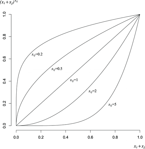
The blending effects corresponding to five different values of s_ij (s_ij = 0.2, 0.5, 1, 2, 5) are shown in Figure 1. Note that increasing s_ij above 1 results in a term whose effect is very small as x_i + x_j approaches zero, while reducing s_ij toward 0 results in a term whose impact decreases rapidly as x_i + x_j approaches zero.

Figure 1 Blending effects for s_ij = 0.2, 0.5, 1, 2, and 5.

Further flexibility can be added by introducing r_ij and r_ji to the model, which gives (9) $$E\left[y\right]=\sum _{i=1}^q{\beta }_i{x}_i+{\beta }_{ij}{\left(\frac{x_i}{x_i+x_j}\right)}^{r_{ij}}{\left(\frac{x_j}{x_i+x_j}\right)}^{r_{ji}}{\left(x_i+x_j\right)}^{s_{ij}},$$(9) where, if s_ij = 1, this is a reduced form of (5(5) $$\begin{array}{ccc}\hfill E\left[y\right]& =& \sum _{i=1}^q{\beta }_i{x}_i+\sum _{i<j}^{q}h\left(x_i,x_j\right)\left(x_i+x_j\right)\hfill \\ & & +\sum _{i<j<k}^{q}h\left(x_i,x_j,x_k\right)\left(x_i+x_j+x_k\right)+\cdots \hfill \end{array}$$(5) ) with only one term of joint effect. Model (9(9) $$E\left[y\right]=\sum _{i=1}^q{\beta }_i{x}_i+{\beta }_{ij}{\left(\frac{x_i}{x_i+x_j}\right)}^{r_{ij}}{\left(\frac{x_j}{x_i+x_j}\right)}^{r_{ji}}{\left(x_i+x_j\right)}^{s_{ij}},$$(9) ) is linear in the parameters β_ij for any values of the parameters s_ij, r_ij, r_ji that define the form of the terms.

This concept can be extended to introduce a general ternary joint effect in the model: (10) $$\begin{array}{ccc}\hfill E\left[y\right]& =& \sum _{i=1}^q{\beta }_i{x}_i+{\beta }_{ijk}{\left(\frac{x_i}{x_i+x_j+x_k}\right)}^{r_{ijk}}{\left(\frac{x_j}{x_i+x_j+x_k}\right)}^{r_{jki}}\hfill \\ & & \times {\left(\frac{x_k}{x_i+x_j+x_k}\right)}^{r_{kij}}{\left(x_i+x_j+x_k\right)}^{s_{ijk}}.\hfill \end{array}$$(10) Here, the joint effect of the x_i, x_j, and x_k is governed by s_ijk, r_ijk, r_jki, r_kij, and the corresponding β_ijk. In particular, s_ijk governs the blending effect between x_i, x_j, and x_k and the remainder of the mixture, in an analogous manner to s_ij above. Thus, contrasting effects may be seen along any ray where x_i, x_j, and x_k remain in fixed relative proportions. The new terms for the binary and ternary cases are referred to as generalized terms of binary and ternary joint effects.

Model (9(9) $$E\left[y\right]=\sum _{i=1}^q{\beta }_i{x}_i+{\beta }_{ij}{\left(\frac{x_i}{x_i+x_j}\right)}^{r_{ij}}{\left(\frac{x_j}{x_i+x_j}\right)}^{r_{ji}}{\left(x_i+x_j\right)}^{s_{ij}},$$(9) ) may alternatively be expressed as $$\begin{array}{ccc}\hfill E\left[y\right]& =& \sum _{i=1}^q{\beta }_i{x}_i+{\beta }_{ij}{\left(\frac{x_i}{x_i+x_j}\right)}^{g_{ij}{h}_{ij}}\hfill \\ & & \times {\left(\frac{x_j}{x_i+x_j}\right)}^{g_{ji}(1-h_{ji})}{\left(x_i+x_j\right)}^{s_{ij}},\hfill \end{array}$$where g_ijh_ij = r_ij and g_ij(1 − h_ij) = r_ji, so that g_ij = r_ij + r_ji and h_ij = r_ij/g_ij. This allows us to better interpret the effects r_ij and r_ji through constrained values of h_ij, g_ij, and g_ji, where 0 ⩽ h_ij ⩽ 1, g_ij > 0 and g_ji > 0.

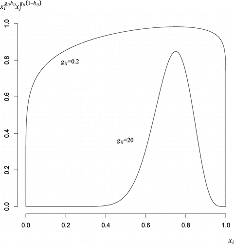
The interpretation of gij, gij, and hij may be understood, without loss of generality, along the edge where xi + xj = 1. First hij describes location, that is the point of greatest departure from linearity, with hij = 0.5 indicating a symmetrical effect. Meanwhile, gij defines the localization of the effect, where gij ≫ 1 indicates a joint effect contained to a region localized about the point of greatest departure from linearity. In contrast, where gij ≪ 1, the effect of the term changes little around this point but instead causes rapid change as xi/(xi + xj) approaches 0 and 1. The effect of the term is proportional to xgijhijixgij(1 − hij)j. To illustrate the way the shape changes with xi (or conversely with 1 − xj), the effects for gij = 20 and gij = 0.2 are shown in Figure 2 for hij = 0.75.

Figure 2 Binary blending effects for g_ij = 0.2 and 20.

A general binary term has no effect when x_i/(x_i + x_j) or x_j/(x_i + x_j) approaches zero. When h_ij = 1 (or conversely, h_ij = 0) the general binary blending term has greater significance as x_i/(x_i + x_j) approaches 1, and x_i dominates the effect. The manner in which this occurs is governed by g_ij. For values of g_ij > 1 the term becomes increasingly influential at an increasingly rapid rate as x_i/(x_i + x_j) approaches 1. For values of g_ij < 1 the term becomes increasingly influential at a decreasingly rapid rate. The impact of the term diminishes for larger values of g_ij. The parameter β_ij sets the magnitude of the effect given its specification by s_ij, g_ij, and h_ij.

Similar analysis may be made of the general term for a ternary joint effect. Model (10(10) $$\begin{array}{ccc}\hfill E\left[y\right]& =& \sum _{i=1}^q{\beta }_i{x}_i+{\beta }_{ijk}{\left(\frac{x_i}{x_i+x_j+x_k}\right)}^{r_{ijk}}{\left(\frac{x_j}{x_i+x_j+x_k}\right)}^{r_{jki}}\hfill \\ & & \times {\left(\frac{x_k}{x_i+x_j+x_k}\right)}^{r_{kij}}{\left(x_i+x_j+x_k\right)}^{s_{ijk}}.\hfill \end{array}$$(10) ) may alternatively be expressed $$\begin{array}{ccc}\hfill E\left[y\right]& =& \sum _{i=1}^q{\beta }_{ijk}{x}_i{x}_j{x}_k{\left(\frac{x_i}{x_i+x_j+x_k}\right)}^{g_{ijk}{h}_{ijk}}\hfill \\ & & \times {\left(\frac{x_j}{x_i+x_j+x_k}\right)}^{g_{ijk}{h}_{jki}}\hfill \\ & & \times {\left(\frac{x_k}{x_i+x_j+x_k}\right)}^{g_{ijk}\left(1-h_{ijk}-h_{jki}\right)}{\left(x_i+x_j+x_k\right)}^{s_{ijk}},\hfill \end{array}$$where g_ijk = r_ijk + r_jki + r_kij, h_ijk = r_ijk/g_ijk, h_jki = r_jki/g_ijk, g_ijkh_ijk = r_ijk, g_ijkh_jki = r_jki, and g_ijk(1 − h_ijk − h_jki) = r_kij. The new terms for the generalized ternary effects can be interpreted in a similar way as the generalized binary effects discussed earlier, without loss of the generality, as the effect of the term across the two-dimensional simplex where x_i + x_j + x_k = 1. The parameters h_ijk and h_jki describe the location of the point of greatest departure from linearity, with h_ijk = h_jki = 1/3 indicating a rotationally symmetrical effect, while g_ijk once again describes the localization of the effect about that point.

3.2 General Blending Mixture Models

We propose a class of generalized blending mixture (GBM) models, for q components, of the form (11) $$\begin{array}{ccc}\hfill E\left[y\right]& =& \sum _{i=1}^q{\beta }_i{x}_i\hfill \\ & & +\sum _{i<j}{\beta }_{ij}{\left(\frac{x_i}{x_i+x_j}\right)}^{r_{ij}}{\left(\frac{x_j}{x_i+x_j}\right)}^{r_{ji}}{\left(x_i+x_j\right)}^{s_{ij}}\hfill \\ & & +\sum _{i<j<k}{\beta }_{ijk}{\left(\frac{x_i}{x_i+x_j+x_k}\right)}^{r_{ijk}}{\left(\frac{x_j}{x_i+x_j+x_k}\right)}^{r_{jki}}\hfill \\ & & \times {\left(\frac{x_k}{x_i+x_j+x_k}\right)}^{r_{kij}}{\left(x_i+x_j+x_k\right)}^{s_{ijk}}.\hfill \end{array}$$(11)

In the second and third sums, we have $\left(\genfrac{}{}{0pt}{}{q}{2}\right)$ and $\left(\genfrac{}{}{0pt}{}{q}{3}\right)$ terms, respectively. Although one could have multiple terms involving the same variables with different powers, we do not consider this.

As discussed earlier, the GBM models can also be reparameterized as (12) $$\begin{array}{ccc}& & E\left[y\right]=\sum _{i=1}^q{\beta }_i{x}_i\hfill \\ & & +\sum _{i<j}{\beta }_{ij}{\left(\frac{x_i}{x_i+x_j}\right)}^{g_{ij}{h}_{ij}}{\left(\frac{x_j}{x_i+x_j}\right)}^{g_{ji}(1-h_{ij})}{\left(x_i+x_j\right)}^{s_{ij}}\hfill \\ & & +\sum _{i<j<k}{\beta }_{ijk}{\left(\frac{x_i}{x_i+x_j+x_k}\right)}^{g_{ijk}{h}_{ijk}}{\left(\frac{x_j}{x_i+x_j+x_k}\right)}^{g_{jki}{h}_{jki}}\hfill \\ & & \times {\left(\frac{x_k}{x_i+x_j+x_k}\right)}^{g_{kij}(1-h_{ijk}-h_{jki})}{\left(x_i+x_j+x_k\right)}^{s_{ijk}}.\hfill \end{array}$$(12)

Models (11(11) $$\begin{array}{ccc}\hfill E\left[y\right]& =& \sum _{i=1}^q{\beta }_i{x}_i\hfill \\ & & +\sum _{i<j}{\beta }_{ij}{\left(\frac{x_i}{x_i+x_j}\right)}^{r_{ij}}{\left(\frac{x_j}{x_i+x_j}\right)}^{r_{ji}}{\left(x_i+x_j\right)}^{s_{ij}}\hfill \\ & & +\sum _{i<j<k}{\beta }_{ijk}{\left(\frac{x_i}{x_i+x_j+x_k}\right)}^{r_{ijk}}{\left(\frac{x_j}{x_i+x_j+x_k}\right)}^{r_{jki}}\hfill \\ & & \times {\left(\frac{x_k}{x_i+x_j+x_k}\right)}^{r_{kij}}{\left(x_i+x_j+x_k\right)}^{s_{ijk}}.\hfill \end{array}$$(11) ) and (12(12) $$\begin{array}{ccc}& & E\left[y\right]=\sum _{i=1}^q{\beta }_i{x}_i\hfill \\ & & +\sum _{i<j}{\beta }_{ij}{\left(\frac{x_i}{x_i+x_j}\right)}^{g_{ij}{h}_{ij}}{\left(\frac{x_j}{x_i+x_j}\right)}^{g_{ji}(1-h_{ij})}{\left(x_i+x_j\right)}^{s_{ij}}\hfill \\ & & +\sum _{i<j<k}{\beta }_{ijk}{\left(\frac{x_i}{x_i+x_j+x_k}\right)}^{g_{ijk}{h}_{ijk}}{\left(\frac{x_j}{x_i+x_j+x_k}\right)}^{g_{jki}{h}_{jki}}\hfill \\ & & \times {\left(\frac{x_k}{x_i+x_j+x_k}\right)}^{g_{kij}(1-h_{ijk}-h_{jki})}{\left(x_i+x_j+x_k\right)}^{s_{ijk}}.\hfill \end{array}$$(12) ) may be used to establish a broad range of joint effects. In fact, many models presented in the literature are special cases of our class of models. For example, the quadratic crossproduct terms in the Scheffé polynomial or the PQM model, occur when h_ij = 0.5, g_ij = 2, and s_ij = 2. The squared terms in the PQM model occur when h_ij = 0, g_ij = 2, and s_ij = 2. The binary blending terms of Becker’s H2 and H3 models occur when h_ij = 0.5, s_ij = 1, and g_ij = 2 or 1, respectively. Furthermore, the ternary term of the special cubic model occurs when $h_{ijk}=h_{jim}=\frac{1}{3}$, g_ijk = 3, and s_ijk = 3. Thus, the GBM model allows us to consider commonly used terms, as well as new terms, with considerable flexibility.

4. MODEL SELECTION

Model (11(11) $$\begin{array}{ccc}\hfill E\left[y\right]& =& \sum _{i=1}^q{\beta }_i{x}_i\hfill \\ & & +\sum _{i<j}{\beta }_{ij}{\left(\frac{x_i}{x_i+x_j}\right)}^{r_{ij}}{\left(\frac{x_j}{x_i+x_j}\right)}^{r_{ji}}{\left(x_i+x_j\right)}^{s_{ij}}\hfill \\ & & +\sum _{i<j<k}{\beta }_{ijk}{\left(\frac{x_i}{x_i+x_j+x_k}\right)}^{r_{ijk}}{\left(\frac{x_j}{x_i+x_j+x_k}\right)}^{r_{jki}}\hfill \\ & & \times {\left(\frac{x_k}{x_i+x_j+x_k}\right)}^{r_{kij}}{\left(x_i+x_j+x_k\right)}^{s_{ijk}}.\hfill \end{array}$$(11) ) is complex, being a nonlinear function of some of its parameters. Its estimation is difficult but possible. However, in most cases it is unnecessary to estimate all its parameters simultaneously. When the parameters r_ij, r_ji, s_ij, r_ijk, r_jik, and s_ijk are specified, the estimation of the remaining parameters of (11(11) $$\begin{array}{ccc}\hfill E\left[y\right]& =& \sum _{i=1}^q{\beta }_i{x}_i\hfill \\ & & +\sum _{i<j}{\beta }_{ij}{\left(\frac{x_i}{x_i+x_j}\right)}^{r_{ij}}{\left(\frac{x_j}{x_i+x_j}\right)}^{r_{ji}}{\left(x_i+x_j\right)}^{s_{ij}}\hfill \\ & & +\sum _{i<j<k}{\beta }_{ijk}{\left(\frac{x_i}{x_i+x_j+x_k}\right)}^{r_{ijk}}{\left(\frac{x_j}{x_i+x_j+x_k}\right)}^{r_{jki}}\hfill \\ & & \times {\left(\frac{x_k}{x_i+x_j+x_k}\right)}^{r_{kij}}{\left(x_i+x_j+x_k\right)}^{s_{ijk}}.\hfill \end{array}$$(11) ) becomes trivial as the resulting models are linear in the parameters. Therefore, a sensible alternative to estimating (11(11) $$\begin{array}{ccc}\hfill E\left[y\right]& =& \sum _{i=1}^q{\beta }_i{x}_i\hfill \\ & & +\sum _{i<j}{\beta }_{ij}{\left(\frac{x_i}{x_i+x_j}\right)}^{r_{ij}}{\left(\frac{x_j}{x_i+x_j}\right)}^{r_{ji}}{\left(x_i+x_j\right)}^{s_{ij}}\hfill \\ & & +\sum _{i<j<k}{\beta }_{ijk}{\left(\frac{x_i}{x_i+x_j+x_k}\right)}^{r_{ijk}}{\left(\frac{x_j}{x_i+x_j+x_k}\right)}^{r_{jki}}\hfill \\ & & \times {\left(\frac{x_k}{x_i+x_j+x_k}\right)}^{r_{kij}}{\left(x_i+x_j+x_k\right)}^{s_{ijk}}.\hfill \end{array}$$(11) ) is to choose a model from a list of models that includes traditional models as well as new GBM models obtained for a grid of values for r_ij, r_ji, s_ij, r_ijk, r_jik, and s_ijk. The model selection criterion $${\text{AIC}}_c=2pn/(n-p+1)-2\text{log}\left(L\right)$$is used, where L is the likelihood function and p is the number of the parameters of the estimated model.

There are various ways of implementing such a comparison. The results presented here were obtained by a forward selection stepwise regression procedure, that is, by fitting first the model including the effects of the individual mixture components and then sequentially adding the best possible term representing joint action of two or three components, defined by all possible values of r_ij, r_ji, s_ij, r_ijk, r_jik, and s_ijk and judged by the AIC_c criterion. The fitting was terminated when the models became unnecessarily complicated. The computer implementation was done with the free software package R using the AICc function of the library AICcmodavg (Mazerolle 2013). The computer program is provided as online supplementary material.

Most published datasets obtained in mixture experiments are provided with satisfactory statistical analyses using standard models. Fitting GBM models to such data, therefore, usually brings modest benefits, which is not surprising. Furthermore, the experimental designs used in such studies often do not allow for fitting the GBM models, as they either have too few observations or their location in the design region does not allow the estimation of some of the model parameters. This is why to illustrate the features of the new models, data were simulated for a scenario where their advantages in comparison with standard models could be seen. Certainly, this is not a typical case and in most practical situations the differences seen in this example are likely to be considerably smaller.

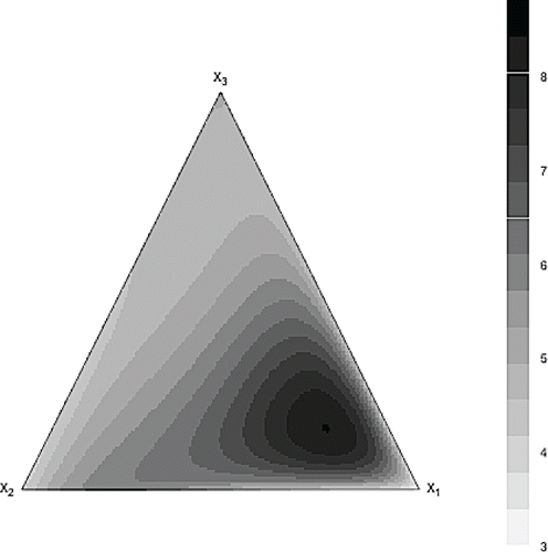
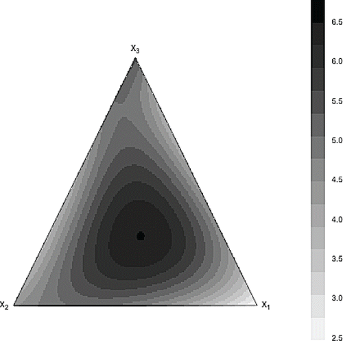
Example. This example involves three mixture components with their proportions varying from 0 to 1. The response surface for this example was chosen to be asymmetric, but ordinary; see Figure 3. The maximum of the response was attained by a combination of a large proportion of x₁ and similar but small proportions of the remaining components x₂ and x₃. However, the joint effect of the mixture components was strong. This was achieved by using the model $$E\left[y\right]=3x_1+4x_2+5x_3+20x_1{x}_2^3+80\frac{x_1^{2.5}{x}_2^{0.5}{x}_3^{0.5}}{x_1+x_2+x_3}.$$

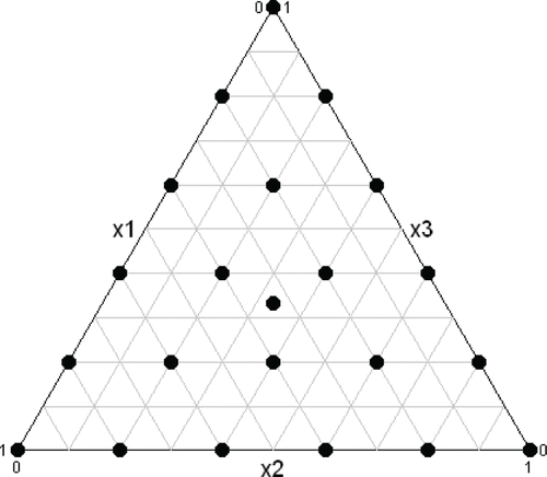
The data were generated for the 22-trial, 3-component simplex lattice design with an additional centroid point shown in Figure 4. Independent and normally distributed random errors with homogeneous variance equal to 0.25² were added to the model-calculated values to yield the simulated data.

Figure 3 Contour plot for the underlying model.

Figure 4 Plot of design for simulated data.

The best GBM model with four terms was chosen by comparing all possible models obtained by adding to the model having just three terms, that is, $$E\left[y\right]=\sum _{i=1}^3{\beta }_i{x}_i,$$a single term of joint action. There were four types of terms to consider adding: ${\beta }_{ij}{\left(\frac{x_i}{x_i+x_j}\right)}^{r_{ij}}{\left(\frac{x_j}{x_i+x_j}\right)}^{r_{ji}}{\left(x_i+x_j\right)}^{s_{ij}}$, for i = 1, j = 2; i = 1, j = 3; and i = 2, j = 3; and β123xr1231xr2312xr3123, where the last term simplified from that in (11(11) $$\begin{array}{ccc}\hfill E\left[y\right]& =& \sum _{i=1}^q{\beta }_i{x}_i\hfill \\ & & +\sum _{i<j}{\beta }_{ij}{\left(\frac{x_i}{x_i+x_j}\right)}^{r_{ij}}{\left(\frac{x_j}{x_i+x_j}\right)}^{r_{ji}}{\left(x_i+x_j\right)}^{s_{ij}}\hfill \\ & & +\sum _{i<j<k}{\beta }_{ijk}{\left(\frac{x_i}{x_i+x_j+x_k}\right)}^{r_{ijk}}{\left(\frac{x_j}{x_i+x_j+x_k}\right)}^{r_{jki}}\hfill \\ & & \times {\left(\frac{x_k}{x_i+x_j+x_k}\right)}^{r_{kij}}{\left(x_i+x_j+x_k\right)}^{s_{ijk}}.\hfill \end{array}$$(11) ) as x1 + x2 + x3 = 1. Each of these terms was considered for all possible combinations of the values 0.5, 1, 1.5, 2, 2.5, or 3 for r12, r13, r23, r123, r231, and r312 and the values 0, 1, 2, or 3 for s12, s13, and s23. Hence, 3(4*62) + 63 = 648 models were considered. The model with smallest AICc was chosen. It included a term representing binary blending for the components x1 and x2.

The best GBM model with five terms was chosen by comparing all models obtained by adding one more term to the best GBM model with four terms. The list of models to compare was obtained in the same way as that used to obtain the best GBM model with four terms. At this stage a term representing ternary blending for the components was included.

The same approach was used again to obtain the best GBM model with six and then, with seven terms. The terms that were added represented binary blending for components x₁ and x₃ and for components x₂ and x₃, respectively. As expected, the model with seven terms had the same structure as (11(11) $$\begin{array}{ccc}\hfill E\left[y\right]& =& \sum _{i=1}^q{\beta }_i{x}_i\hfill \\ & & +\sum _{i<j}{\beta }_{ij}{\left(\frac{x_i}{x_i+x_j}\right)}^{r_{ij}}{\left(\frac{x_j}{x_i+x_j}\right)}^{r_{ji}}{\left(x_i+x_j\right)}^{s_{ij}}\hfill \\ & & +\sum _{i<j<k}{\beta }_{ijk}{\left(\frac{x_i}{x_i+x_j+x_k}\right)}^{r_{ijk}}{\left(\frac{x_j}{x_i+x_j+x_k}\right)}^{r_{jki}}\hfill \\ & & \times {\left(\frac{x_k}{x_i+x_j+x_k}\right)}^{r_{kij}}{\left(x_i+x_j+x_k\right)}^{s_{ijk}}.\hfill \end{array}$$(11) ).

It may be beneficial to use different blending terms for the same components only in very rare situations. If this possibility is excluded in the model selection, it becomes faster as the number of models to consider becomes smaller as more terms are added to the model.

The full Scheffé cubic polynomial (2(2) $$\begin{array}{ccc}\hfill E\left[y\right]& =& \sum _{i=1}^q{\beta }_i{x}_i+\sum _{i\ne j}^q{\beta }_{ij}{x}_i{x}_j,\hfill \\ \hfill E\left[y\right]& =& \sum _{i=1}^q{\beta }_i{x}_i+\sum _{i<j}^q{\beta }_{ij}{x}_i{x}_j\hfill \\ & & +\sum _{i<j}^q{\gamma }_{ij}{x}_i{x}_j(x_i-x_j)+\sum _{i<j<k}^q{\beta }_{ijk}{x}_i{x}_j{x}_k,\hfill \end{array}$$(2) ), Becker’s models H2 (3(3) $$\begin{array}{ccc}\hfill \mathrm{H}1:E\left[y\right]& =& \sum _{i=1}^q{\beta }_i{x}_i+\sum _{i<j}^q{\beta }_{ij}min\left(x_i,x_j\right)\hfill \\ & & +\sum _{i<j<k}^q{\beta }_{ijk}min\left(x_i,x_j,x_k\right)+\cdots ,\hfill \\ \hfill \mathrm{H}2:E\left[y\right]& =& \sum _{i=1}^q{\beta }_i{x}_i+\sum _{i<j}^q{\beta }_{ij}\frac{x_i{x}_j}{x_i+x_j}\hfill \\ & & +\sum _{i<j<k}^q{\beta }_{ijk}\frac{x_i{x}_j{x}_k}{x_i+x_j+x_k}+\cdots ,\hfill \end{array}$$(3) ) and H3 (4(4) $$\begin{array}{ccc}\hfill \mathrm{H}3:E\left[y\right]& =& \sum _{i=1}^q{\beta }_i{x}_i+\sum _{i<j}^q{\beta }_{ij}\sqrt{x_i{x}_j}\hfill \\ & & +\sum _{i<j<k}^q{\beta }_{ijk}\sqrt{3x_i{x}_j{x}_k}+\cdots .\hfill \end{array}$$(4) ) were also fitted to the data. Their AIC_c statistics, as well as those for the best GBM models with three, four, five, six, and seven terms, are given in Table 1.

Table 1 AIC_c statistics for models fitting the simulated data

Model	Scheffé	H2	H3	GBM	GBM	GBM	GBM	GBM
Terms	10	7	7	3	4	5	6	7
AICc	95.85	80.53	78.72	80.60	45.53	9.91	10.49	11.81

The GBM model with five terms had a smaller AIC_c statistic than those for the GBM models with three, four, six, or seven terms, and was overall the best model. This model is $$\begin{array}{ccc}\hfill \widehat{y}& =& 2.8791(0.1366)x_1+3.8191(0.1585)x_2+5.1871(0.1279)x_3\hfill \\ & & +19.628(2.1260)x_1{x}_2^2+82.3909(3.6170)\frac{x_1^{2.5}{x}_2^{0.5}{x}_3^{0.5}}{x_1+x_2+x3},\hfill \end{array}$$where the figures in the brackets are the standard deviations of the estimates of the parameters that precede them. The AIC_c value for this model is 9.91 and compares rather favorably with the corresponding values for the fitted full Scheffé cubic polynomial and Becker’s H2 and H3 models for which it is 95.85, 80.53, and 78.72, respectively. While we emphasize that such advantageous differences in favor of the GBM models are not typical, this example shows that for certain studied phenomena they can be achieved.

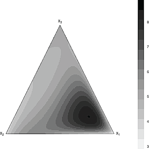
The contour plots of the predicted surfaces with the full Scheffé cubic polynomial and the selected GBM model are shown in Figures 5 and 6. It can be seen that the estimated response surfaces of the GBM model was very similar to the true response surface shown in Figure 3. This cannot be said for the estimated full Scheffé cubic polynomial as its estimated response surface is notably different from the true surface.

Figure 5 Prediction contour plot for Scheffé special cubic model fit to the simulated data.

Figure 6 Prediction contour plot for GBM model fit to the simulated data.

Using a grid with a larger number of possible values for r₁₂, r₁₃, r₂₃, r₁₂₃, r₂₃₁, r₃₁₂, s₁₂, s₁₃, and s₂₃ was attempted but did not bring any benefits. It was felt that the reason for that was that the amount of simulated data was not sufficiently large to allow to distinguish between models with such small differences of the values of the nonlinear parameters. However, as different models were found, some with structures somewhat different to that of the true model, they all produced predictions which would be considered indistinguishable in a practical application and well representing the underlying relationship.

5. DISCUSSION

The general class of models that we propose, provide a powerful unification and extension of the existing statistical methodology for analysis of data obtained in mixture experiments. The complexity of the models fitted to the data will closely match the complexity of the studied phenomena: they will be models equivalent to those proposed by Scheffé (1958, 1963), Becker (1968), and Piepel, Szychowski, and Loeppky (2002) when possible, but more complex when needed. The main benefits of using GBM models are that they are parsimonious and can accurately describe response surfaces in situations where sometimes standard models will offer only a crude and possibly even misleading approximation.

Estimating simultaneously all parameters of the GBM models (11(11) $$\begin{array}{ccc}\hfill E\left[y\right]& =& \sum _{i=1}^q{\beta }_i{x}_i\hfill \\ & & +\sum _{i<j}{\beta }_{ij}{\left(\frac{x_i}{x_i+x_j}\right)}^{r_{ij}}{\left(\frac{x_j}{x_i+x_j}\right)}^{r_{ji}}{\left(x_i+x_j\right)}^{s_{ij}}\hfill \\ & & +\sum _{i<j<k}{\beta }_{ijk}{\left(\frac{x_i}{x_i+x_j+x_k}\right)}^{r_{ijk}}{\left(\frac{x_j}{x_i+x_j+x_k}\right)}^{r_{jki}}\hfill \\ & & \times {\left(\frac{x_k}{x_i+x_j+x_k}\right)}^{r_{kij}}{\left(x_i+x_j+x_k\right)}^{s_{ijk}}.\hfill \end{array}$$(11) ) would require a substantial computational effort. The authors have made considerable progress in developing a computational tool capable of doing this, though its discussion remains outside the scope of the presented research. However, the method of choosing a GBM model proposed in this article is effective, simple, and computationally stable, thus it is good for its purpose.

The development of the general class of mixture models naturally creates the need to reevaluate the usefulness of the standard and computer generated experimental designs for mixture experiments. It is clear that fitting GBM models requires more data than fitting any of the standard models. It is possible to use space-filling experimental designs, collecting as much data as the available resources allow for. Such designs have been explored, for example, by Fang and Wang (1994), Borkowski and Piepel (2009), and Ning, Fang, and Zhou (2011). Further work aiming to formulate a better experimental design strategy for estimating the class of general blending mixture models that takes into account their structure is underway.

SUPPLEMENTARY MATERIALS

Data and Code: The simulated dataset used in the example in Section 4 of the article, along with R code to perform the analysis (zip folder).

ACKNOWLEDGMENTS

We were fortunate to have our article been refereed by an Editor, Associate Editor, and the two referees who understand well the theory and practice of mixture experiments. Their extensive and constructive suggestions were invaluable to us in the revisions of this article.

References

- Atkinson, A.C., Donev, A.N., and Tobias, R. (2007), Optimum Experimental Designs, with SAS, New York: Oxford University Press.
- Becker, N.G. (1968), “Models for the Response of a Mixture,” Journal of the Royal Statistical Society, Series B, 30, 349–358.
- Becker, N.G. (1970), “Mixture Designs for a Model Linear in the Proportions,” Biometrika, 57, 329–338.
- Becker, N.G. (1978), “Models and Designs for Experiments With Mixtures,” Australian Journal of Statistics, 20, 195–208.
- Borkowski, J.J., and Piepel, G.F. (2009), “Uniform Designs for Highly Constrained Mixtures Experiments,” Journal of Quality Technology, 41, 35–47.
- Chen, J.J., Li, L.A., and Jackson, C.D. (1996), “Analysis of Quantal Response Data From Mixture Experiments,” Environmetrics, 7, 503–512.
- Chen, W.S., Zhu, W.Y., and Hu, C.J. (1985), “A New Mixture Model With Three or Four Components and Their Quasi D-optimality,” technical report, Northern Illinois University.
- Claringbold, P.J. (1955), “Use of the Simplex Design in the Study of Joint Action of Related Hormones,” Biometrics, 11, 174–185.
- Cornell, J.A. (2000), “Fitting a Slack-Variable Model to Mixture Data: Some Questions Raised,” Journal of Quality Technology, 32, 133–147.
- Cornell, J.A. (2002), Experiments with Mixtures: Designs, Models, and the Analysis of Mixture Data (3rd ed.), New York: Wiley.
- Darroch, J.N., and Waller, J. (1985), “Additivity and Interaction in Three-Component Experiments With Mixtures,” Biometrika, 72, 153–163.
- Draper, N.R., and John, R. C.S. (1977a), “Designs in Three and Four Components for Mixtures Models With Inverse Terms,” Technometrics, 19, 117–130.
- Draper, N.R. (1977b), “A Mixtures Model With Inverse Terms,” Technometrics, 19, 37–46.
- Draper, N.R., and Lawrence, W. (1965a), “Mixture Designs for Four Factors,” Journal of the Royal Statistical Society, Series B, 27, 473–478.
- Draper, N.R. (1965b), “Mixture Designs for Three Factors,” Journal of the Royal Statistical Society, Series B, 27, 450–465.
- Draper, N.R., and Pukelsheim, F. (1998), “Mixture Models Based on Homogeneous Polynomials,” Journal of Statistical Planning and Inference, 71, 303–311.
- Efroymson, M.A. (1965), “Multiple Regression Analysis,” in Mathematical Methods for Digital Computers, eds. A. Ralston and H. S. Wilf, New York: Wiley.
- Fang, K.-T., and Wang, Y. (1994), Number Theoretic Methods in Statistics, London: Chapman and Hall.
- Focke, W.W., Ackermann, M.H., and Coetzer, R. L.J. (2012), “Mixing Rules Based on Power Means and Generalized q-fractions,” Journal of Chemical Engineering of Japan, 45, 1–8.
- Focke, W.W., Sandrock, C., and Kok, S. (2007), “Weighted-Power-Mean Mixture Model: Application to Multicomponent Liquid Viscosity,” Industrial Engineering Chemistry Research, 46, 4660–4666.
- Gorman, J.W., and Hinman, J.E. (1962), “Simplex Lattice Designs for Multicomponent Systems,” Technometrics, 4, 463–487.
- Hackler, W.C., Kriegel, W.W. and Hader, R.J. (1956), “Effect of Raw-Material Ratios on Absorption of Whiteware Compositions,” Journal of the American Ceramic Society, 39, 20–25.
- Johnson, T.M., and Zabik, M.E. (1981), “Response Surface Methodology for Analysis of Protein Interactions in Angel Food Cakes,” Journal of Food Science, 46, 1226–1230.
- Kenworthy, O.O. (1963), “Fractional Experiments With Mixtures Using Ratios,” Industrial Quality Control, 19, 24–26.
- Mazerolle, M.J. (2013), AICcmodavg: Model Selection and Multimodel Inference Based on (Q)AIC(c), R package version 1.35.
- Ning, J.-H., Fang, K.-T., and Zhou, Y.-D. (2011), “Uniform Design for Experiments With Mixtures,” Communications in Statistics—Theory and Methods, 40, 1734–1742.
- Piepel, G.F., Szychowski, J.M., and Loeppky, J.L. (2002), “Augmenting Scheffe Linear Mixture Models With Squared and/or Crossproduct Terms,” Journal of Quality Technology, 34, 297–314.
- Quenouillé, M.H. (1953), The Design and Analysis of Experiments, New York: Hafner.
- Quenouillé, M.H. (1959), “Experiments With Mixtures,” Journal of the Royal Statistical Society, Series B, 21, 201–202.
- Quenouillé, M.H. (1963), Discussion of “The Simplex-Centroid Design for Experiments With Mixtures” by H. Scheffé, Journal of the Royal Statistical Society, Series B, 25, 235–263.
- Scheffé, H. (1958), “Experiments With Mixtures,” Journal of the Royal Statistical Society, Series B, 20, 344–360.
- Scheffé, H. (1963), “The Simplex-centroid Design for Experiments With Mixtures,” Journal of the Royal Statistical Society, Series B, 25, 235–263.
- Snee, R.D. (1973), “Techniques for the Analysis of Mixture Data,” Technometrics, 15, 517–528.
- Thompson, W., and Myers, R. (1968), “Response Surface Designs for Experiments With Mixtures,” Technometrics, 10, 739–756.