Constructing D-Efficient Mixed-Level Foldover Designs Using Hadamard Matrices

Abstract

This paper introduces a new class of Hadamard matrix-based mixed-level foldover designs (MLFODs) and an algorithm which facilitates the construction of MLFODs. Our new MLFODs were constructed by converting some 2-level columns of a Hadamard matrix to 3-level ones. Like the 2-level foldover designs (FODs), each new MLFOD was constructed by a half fraction and its foldover. Our Hadamard-matrix based MLFODs are compared with the conference matrix-based FODs of Jones & Nachtsheim (2013) in terms of the D-efficiencies and the maximum of the absolute values of the correlation coefficients among the columns of the model matrix. Like the latter, our designs are also definitive in the sense that the estimates of all main effects are unbiased with respect to any active second order effects. In addition, they require fewer runs and can be used to study the presence of the second-order effects more efficiently. Examples illustrating the use of our new MLFODs are given.

Keywords:

• Augmented designs
• Conference matrix
• Definitive screening designs
• D-efficiency
• Interchange algorithm
• Plackett-Burman designs

1 Introduction

Foldover is an experimental design technique used when a fractional factorial design (FFD) such as a resolution III FFD, a Hadamard matrix or a Plackett-Burman design produces ambiguous results. Let us call this fraction D. A foldover design (FOD) constructed from this half fraction is of the form: (1) $$\left(\begin{array}{c}\hfill \mathbf{D}\\ \hfill -\mathbf{D}\end{array}\right).$$(1)

FODs form an important class of screening designs. The 2-level FODs have been discussed in most textbooks on design of experiments such as Mee (2009) and Montgomery (2017). The recent paper of Errore et al. (2017) discusses a fast method of constructing 2-level FODs and provides some useful references on 2-level FODs.

To construct the mixed-level FOD (MLFOD), Jones & Nachtsheim (2013) (hereafter abbreviated as JN) constructed the half fraction in (1) by converting some 3-level columns of a conference matrix to 2-level ones. See Jones & Nachtsheim (2011), Xiao et al. (2012) and Nguyen & Stylianou (2013) for the information on conference matrices, orthogonal $(0,\pm 1)$-matrices with zero diagonal and their use in the construction of definitive screening designs (DSDs). These DSDs are 3-level FODs. JN’s conference matrix-based approach was directed to design problems that contain a relatively small number of 2-level factors. JN called their method DSD-augmented method and in this paper we call JN’s MLFOD designs as ADSDs. Note that unlike ADSDs, JN’s designs constructed by their ORTH-augmented method and its extension (see Nachtsheim, et al., 2017) are not MLFODs.

Both DSDs and ADSDs have the following properties: (i) Unlike resolution III designs, all main effects (MEs) are orthogonal to the 2-factor interactions (2FIs); (ii) Unlike the 2-level designs, all quadratic effects are estimable and are orthogonal to the MEs; and (iii) Unlike the 2-level designs, a DSDs or ADSD might render the follow-up experiment unnecessary as it might collapse into a second-order design in a subset of significant factors. An example of collapsing a DSD into a second-order design was given in a set of slides entitled “Creating and Analyzing Definitive Screening Designs” by Tom Donnelly (https://community.jmp.com/t5/Mastering-JMP/Definitive-Screening-Designs-Slides/ta-p/23255).

The only limitation ADSDs have is that as the number between 2-level factors increases, the correlation between the quadratic effects increases. JN p. 129 showed that this correlation was $\frac{1}{2}-\frac{2}{n-4}$ where n is the number of runs. It can be seen that this correlation approaches 0.5 as n becomes large. JN in their paper hinted the development of alternative designs that reduce these correlations.

This paper introduces a Hadamard matrix-based approach to mixed-level methodology. This approach is geared towards design problems that contain a relatively small number of 3-level factors. With this approach, we construct the half fraction in (1) by converting some 2-level columns of a Hadamard matrix or a Plackett-Burman design (Plackett & Burman, 1946) to 3-level ones. See Hedayat & Wallis (1978) for the information on Hadamard matrices and their use in design construction. Our MLFODs not only retain the mentioned properties of ADSDs but also address the limitation of ADSDs mentioned in the previous paragraph.

2 Structure of the x′x matrix of an MLFOD

Let X be the expanded design matrix of an MLFOD with m₃ 3-level factors and m₂ 2-level factors in n (= 2m) runs of a design for the pure quadratic model with p parameters $(p=1+2m_3+m_2)$. This design matrix was constructed by (1) using the half fraction $\mathbf{D}=(d_{\mathit{ij}})$ which has m rows and $m_3+m_2$ columns ($m_3+m_2\le m$). Now, let the i-th row of X be written as $(1,d_{i1}^2,\dots ,d_{i{m}_3}^2,d_{i1},\dots ,d_{i{m}_3},d_{i(m_3+1)},\dots ,d_{i(m_3+m_2)})$. Due to the foldover structure of the design, its information matrix ${\mathbf{X}}^{\prime }\mathbf{X}$ will be of the form (2) $$2\left(\begin{array}{cc}\mathbf{A}\hfill & 0^{\prime }\hfill \\ 0\hfill & \mathbf{B}\hfill \end{array}\right),$$(2) where A is a matrix of size $(1+m_3)\times (1+m_3)$, B a matrix of size $(m_3+m_2)\times (m_3+m_2)$ and 0 a matrix of 0’s.

Assuming each of the m₃ 3-level columns of the half fraction has a fixed number x of 0’s and b = m – x number of ±1’s, the matrix A will be of the form (3) $$\left(\begin{array}{cc}m& b{1}^{\prime }\\ b1& {\mathbf{A}}^{*}\end{array}\right)$$(3) where 1 is a column vector of 1’s and ${\mathbf{A}}^{\ast }$ the core of A in (3), i.e., the matrix A without its first row and first column.

From and (2) and (3), the determinant of ${\mathbf{X}}^{\prime }\mathbf{X}$ for the pure quadratic model can be computed as (4) $$\left|{\mathbf{X}}^{\prime }\mathbf{X}\right|=2^{1+2m_3+m_2} m |{\mathbf{A}}^{*}-\frac{b^2}{m} \mathbf{J}| \left|\mathbf{B}\right|.$$(4)

Here J is a matrix of 1’s. In this paper, we will maximize $\left|{\mathbf{X}}^{\prime }\mathbf{X}\right|$ in (4) by maximizing $|{\mathbf{A}}^{*}-\frac{b^2}{m} \mathbf{J}|$ and $\left|\mathbf{B}\right|$ by the approximate approach. Let λ_i ’s be the eigenvalues of a symmetric matrix of full rank. Note that the trace of this matrix is $\sum {\lambda }_i$ and sum of the squares of the elements of this matrix is $\sum {\lambda }_i^2$. Thus if the trace of this matrix is constant, minimizing the sum of the squares of the off-diagonal elements of this matrix is the same as making the λ_i as equal as possible with $\sum {\lambda }_i$ being constant. This is the same as maximizing the determinant of this matrix, i.e., $\Pi {\lambda }_i$. Since the diagonal elements of ${\mathbf{A}}^{*}-\frac{b^2}{m} \mathbf{J}$ and B and their traces $m_3 (b-\frac{b^2}{m})$ and $m_{3}b+m_{2}m$ respectively, are constant, we can maximize $|{\mathbf{A}}^{*}-\frac{b^2}{m} \mathbf{J}|$ and $\left|\mathbf{B}\right|$ by minimizing the sum of the squares of the off-diagonal elements of these two matrices. This is also the approach which Nguyen (1996) used to obtain efficient supersaturated designs.

For the main effect model, the expanded design matrix X does not include the pure quadratic effects, and the determinant of ${\mathbf{X}}^{\prime }\mathbf{X}$ can be computed as (5) $$\left|{\mathbf{X}}^{\prime }\mathbf{X}\right|=2^{1+m_3+m_2} m \left|\mathbf{B}\right|.$$(5)

In this paper, we are particularly interested in MLFODs having the matrix ${\mathbf{A}}^{*}$ in (3) of the form $c \mathbf{J}+d \mathbf{I}$, where I is the identity matrix. We denote this class of MLFODs as MLFOD*s. The ${\mathbf{A}}^{*}$ matrices of DSDs, ADSDs and popular second-order designs are all of this form. For an MLFOD*, $|{\mathbf{A}}^{*}-\frac{b^2}{m} \mathbf{J}|$ in (4) can be easily calculated and ${\mathbf{A}}^{-1}$, the inverse of A in (3), will have the form (6) $$\left(\begin{array}{cc}p& q{1}^{\prime }\\ q1& s\mathbf{J}+t\mathbf{I}\end{array}\right),$$(6) where $p=(m_{3}c+d)/a, q=-b/a, s=(b^2-\mathit{mc})/\mathit{da}, t=1/d$, and $a=m(m_{3}c+d)-m_3{b}^2$ (see P. W. M. John, 1971, section 10.2 on Second-Order Designs). Thus, the covariance between quadratic effects of an MLFOD* is a constant. Note that if $c=\frac{b^2}{m}$ then s = 0 and the quadratic effects are orthogonal to one another.

Desirable design properties such as those of DSDs and ADSDs mentioned in the Introduction or the one of MLFOD*s and popular second-order designs mentioned in the previous paragraph simplify the data analysis and interpretation of the results. While computation simplicity is not much of our concern nowadays, ease of the interpretation of the results is very much welcome by experimenters. In the next section, we will introduce an algorithm for constructing MLFOD*s with $c=[\frac{b^2}{m}]$ where $[·]$ is the rounding function.

3 The FOLDOVER algorithm

Our approach for constructing the half fraction in (1) of an MLFOD* with m₃ 3-level factors and $m_2$ 2-level factors is to select $m_3+m_2$ columns of a Hadamard matrix of order $m (m_3+m_2\le m)$ and then convert the first m₃ 2-level columns of this matrix to 3-level ones. If m is not a multiple of four and a Hadamard matrix or a Plackett-Burman design is not available, FOLDOVER could use the matrices of maximal determinant, e.g. those in http://www.indiana.edu/∼maxdet/. Although these matrices of maximal determinant do not guarantee zero correlation among 2-level columns, they do guarantee minimum correlation among them. Let’s call the input matrix $\mathbf{D}=(d_{\mathit{ij}})$.

We use the i-th row of D to construct the vector ${\mathbf{K}}_i$ of length $2{(}_{ 2}^{m_3})+m_3{m}_2$. The first ${(}_{ 2}^{m_3})$ entries of ${\mathbf{K}}_i$ are $d_{i1}^2{d}_{i2}^2,\dots ,d_{i(m_3-1)}^2{d}_{i{m}_3}^2$. The next ${(}_{ 2}^{m_3})$ entries are $d_{i1}{d}_{i2},\dots ,d_{i(m_3-1)}{d}_{i{m}_3}$. The last $m_3{m}_2$ entries are $d_{i1}{d}_{i(m_3+1)},\dots ,d_{i{m}_3}{d}_{i(m_3+m_2)}$.

Now, let $\mathbf{K}=\sum {\mathbf{K}}_i$. Subtract $\frac{b^2}{m}$ from each of the first ${(}_{ 2}^{m_3})$ elements of K. Recall that each of the m₃ 3-level columns of the half fraction will have a fixed number x of 0’s and $b=m-x$ number of ±1’s. Let f be the sum of the squares of the first ${(}_{ 2}^{m_3})$ elements of K and g the sum of the squares of the remaining elements of K. It can be easily seen that the lower bound of f is $f^{*}={(}_{ 2}^{m_3}){([\frac{b^2}{m}]-\frac{b^2}{m})}^2$ and the lower bound of g is zero.

Following are the steps of the FOLDOVER algorithm for constructing the half fraction in (1) of an MLFOD* with m₃ 3-level factors and m₂ 2-level factors using vector K:

1. Randomly select $m_3+m_2$ columns from the input matrix D of order $m (m_3+m_2\le m)$. For each row i of D, randomly multiply each of the elements of this row by –1 (or leave it intact). Randomly set x elements of each of the first m₃ columns of D to 0. Calculate each ${\mathbf{K}}_i, (i=1,\dots ,n)$ and $\mathbf{K}=\sum {\mathbf{K}}_i$. Subtract $\frac{b^2}{m}$ from each of the first ${(}_{ 2}^{m_3})$ elements of K. Calculate the f and g values.

2. Search for a pair of entries in column $j (j=1\dots ,m_3)$ of D such that the swap of these two entries will result in the biggest reduction in f (or g if f cannot be reduced further). If the search is successful, update $f, g, \mathbf{K}$ and column j. If f (or g if f cannot be reduced further) cannot be reduced further, repeat this step with the next 3-level column. Repeat this step until the $(f, g)$ values cannot be reduced further by any further swaps.

Remarks:

1. In Step 2, let ${\mathbf{D}}_1$ and ${\mathbf{D}}_2$ be two half fractions with the objective functions (f₁, g₁) and (f₂, g₂). The half fraction ${\mathbf{D}}_2$ is preferred over ${\mathbf{D}}_1$ if $f_2<f_1$ or if f₂ = f₁ and $g_2<g_1$.

2. Steps 1 and 2 make up a try. Among all tries which result in a set of MLFODs whose f’s reach its bound (i.e., $f=f^{*}$) or a minimum (i.e., $f>f^{*}$) we find a subset with the minimum $r_{\text{max}}$ (the maximum absolute correlation among the columns of the model matrix). In this subset, we then select the one with the maximum $\left|{\mathbf{X}}^{\prime }\mathbf{X}\right|$ in (4) . Our stopping rule for each try is when both f and g reach their bound.

3. For most values of m and x, when f reaches its bound, we obtain an MLFOD* solution. However, for certain values of m and x, we have $\frac{b^2}{m}$ as a middle value between $[\frac{b^2}{m}]$ and $[\frac{b^2}{m}]+1$ (e.g. $m=8, x=2, b=6, \frac{b^2}{m}=4.5$). In these cases when f reaches its bound, we either have an MLFOD* or non-MLFOD* solution. Often, the non-MLFOD* has larger $\left|{\mathbf{X}}^{\prime }\mathbf{X}\right|$. However, it is the MLFOD* that we choose.

4. Instead of using f as the primary objective function and g as the secondary objective function as in Step 2, we can swap the roles of these two objective functions. This does not often lead to MLFOD*s but occasionally lead to highly D-efficient MLFOD*s.

5. To make a 2-level factor of an MLFOD a blocking factor, we can simply multiply all elements of rows of the resulting fraction which correspond to the level –1 by –1 before folding over this fraction.

Figure 1 shows the steps for constructing a half fraction of an MLFOD* for three 3-level factors and four 2-level factors in 16 runs ($m_3=3, m_2=4)$ using a Hadamard matrix of order m = 8 and x was set to 2. Figures 1 (a), 1 (b) and 1 (c) correspond to Step 1. Figure 1 (a) shows seven columns of the input matrix D, randomly selected to form a Hadamard matrix. Figure 1 (b) shows some rows of D multiplied with –1. Figure 2 (c) shows two 0’s randomly inserted into each of the first three columns of D. At the end of Step 1, (f, g) values are (0.75, 21). Figures 1 (d) and 1 (e) correspond to Step 2. Figure 1 (d) shows the swap of the second and the eighth elements of the first column, after which (f, g) values have been changed to (0.75, 12). Figure 1 (e) shows the swap of the fifth and the eighth elements of the second column, after which (f, g) values have reached their bounds (0.75, 0). After these two swaps, the matrix A* of the half fraction D in Figure 1 (e) has the form 2I + 4J and the matrix B has the form diag(6, 6, 6, 8, 8, 8, 8).

Figure 1 Steps of the FOLDOVER algorithm in constructing an MLFOD* for three 3-level factors and four 2-level factors in 16 runs.

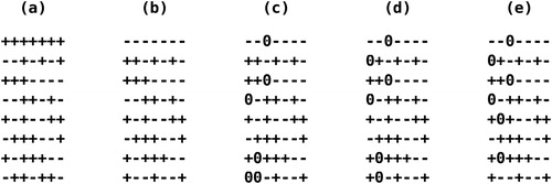
Figure 2 Correlation between two quadratic effects in terms of absolute value of (1) ADSDs, (2) MLFOD*(2), (3) MLFOD*($[\frac{m}{3}]$), (4) MLFOD*($[\frac{m}{4}]$) and (5) MLFOD*($[\frac{m}{5}]$) for various values of $m=8,10,\dots ,100$.

4 Results and Discussion

To compare two MLFODs for a given set of (m₃, m₂), we use the following measures of goodness of a design: d₁, the first-order D-efficiency; d₂, the second-order D-efficiency and $r_{\max }$. The D-efficiencies are calculated as (7) $$|{\mathbf{X}}^{\prime }\mathbf{X}{|}^{1/p}/n,$$(7) where X is the model matrix, p the number of parameters in the model and n the run size of each design. For the first-order model, $\left|{\mathbf{X}}^{\prime }\mathbf{X}\right|$ of our MLFODs is calculated as in (5) and $p=1+m_3+m_2$. For the second-order model, $\left|{\mathbf{X}}^{\prime }\mathbf{X}\right|$ of our MLFODs is calculated as in (4) and $p=1+2m_3+m_2$. Note that the D-efficiencies calculated as in (7) is a measure of information per point. They allow comparisons of designs with different number of design points or runs (cf. Draper & Lin, 1990).

The MLFODs in this study were constructed from the Hadamard matrices and matrices of maximal determinant of order $m=8,10,\dots ,30$ (see http://www.indiana.edu/∼maxdet/). For each m we consider m – 1 sets of (m₃, m₂) with $m_3=1,\dots ,m-1$ and $m_2=m-m_3$. Altogether, we have 216 sets of (m₃, m₂). For each set, we use FOLDOVER to construct an MLFOD(2), an MLFOD($[\frac{m}{3}]$), an MLFOD($[\frac{m}{4}]$) and an MLFOD($[\frac{m}{5}]$) where the number in the brackets refers to the number of 0’s in each of the m₃ 3-level columns of the half fraction in (1). The run size of each MLFOD is $n=2m$. The ADSDs counterparts were constructed by conference matrices of the same order m. The run size of each ADSD is $2(m+1)$.

Here are our main observations: (i) Unlike ADSDs, MLFOD* solutions for a set of (m₃, m₂) mentioned in the previous paragraph can only easily found when $m_3<\frac{m}{2}$ (i.e., $m_3<m_2$). They are much more difficult to find when $m_3\ge \frac{m}{2}$. The off-diagonal elements of the ${\mathbf{A}}^{*}$ matrices of our non-MLFOD* solutions often take two values c and c + 1. (ii) The d₁ of our MLFODs are lower than those of the corresponding ADSDs. The exception is MLFOD(2)s which compete well with ADSDs in terms of d₁. (iii) The d₂ of our MLFODs are higher than those of the corresponding ADSDs; (iv) The r_max values of our MLFOD*s are much smaller than those of the corresponding ADSDs.

Table 1 displays $d_1, d_2$ and r_max values of MLFOD*(2), an MLFOD*($[\frac{m}{5}]$) and ADSDs for 102 sets of (m₃, m₂) with $m_3\le \frac{m}{2}$. Note that $[\frac{m}{5}]$ is two for m = 8, 10 and 12, three for m = 14 and 16, four for m = 18, 20 and 22, five for m = 24 and 26, and six for m = 28 and 30. The $d_1, d_2$ and $r_{\max }$ values of MLFOD*s which are more favorable to the ones of ADSDs are printed in boldface. The construction of 102 MLFOD*(2)’s (each with 5,000 tries) in Table 1 requires 107 minutes on a laptop with Intel(R) Core(TM) i7-3820QM CPU @ 2.70GHz and 102 MLFOD*($[\frac{m}{5}]$) (each with 5,000 tries) in this table requires about two and a half hours and 102 ADSDs (each with 5,000 tries) in this table requires less than three minutes on the same laptop.

Table 1 Comparison of D-efficiencies and r_max of MLFOD*’s and ADSDs.

				MLFOD*(2)				MLFOD*($[\frac{m}{5}]$)				ADSD
n†	m3	m2		d1	d2	rmax		d1	d2	rmax		d1	d2	rmax
16	1	7		0.938	0.799	0.289		0.938	0.799	0.289		0.941	0.794	0.126
16	2	6		0.901	0.670	0.333		0.901	0.670	0.333		0.912	0.666	0.357
16	3	5		0.880	0.572	0.333		0.880	0.572	0.333		0.885	0.572	0.357
20	1	9		0.915	0.791	0.224		0.915	0.791	0.224		0.925	0.795	0.273
20	2	8		0.899	0.686	0.250		0.899	0.686	0.250		0.917	0.684	0.389
20	3	7		0.898	0.610	0.250		0.898	0.610	0.250		0.905	0.597	0.389
20	4	6		0.885	0.535	0.250		0.885	0.535	0.250		0.895	0.529	0.389
24	1	11		0.972	0.846	0.183		0.972	0.846	0.183		0.964	0.836	0.084
24	2	10		0.951	0.734	0.200		0.951	0.734	0.200		0.950	0.720	0.409
24	3	9		0.935	0.648	0.200		0.935	0.648	0.200		0.937	0.629	0.409
24	4	8		0.926	0.580	0.200		0.926	0.580	0.200		0.925	0.557	0.409
24	5	7		0.910	0.514	0.200		0.910	0.514	0.200		0.913	0.499	0.409
28	1	13		0.946	0.833	0.154		0.939	0.843	0.242		0.943	0.827	0.200
28	2	12		0.938	0.737	0.167		0.919	0.751	0.242		0.938	0.725	0.423
28	3	11		0.928	0.659	0.167		0.902	0.680	0.242		0.932	0.640	0.423
28	4	10		0.923	0.596	0.167		0.884	0.620	0.242		0.928	0.573	0.423
28	5	9		0.919	0.542	0.167		0.857	0.565	0.242		0.923	0.517	0.423
28	6	8		0.908	0.488	0.167		0.828	0.519	0.242		0.919	0.471	0.423
32	1	15		0.984	0.871	0.134		0.976	0.880	0.208		0.975	0.861	0.063
32	2	14		0.971	0.771	0.143		0.954	0.785	0.208		0.966	0.755	0.433
32	3	13		0.961	0.691	0.143		0.936	0.710	0.208		0.958	0.669	0.433
32	4	12		0.952	0.626	0.143		0.919	0.648	0.208		0.951	0.598	0.433
32	5	11		0.946	0.571	0.143		0.901	0.595	0.208		0.944	0.539	0.433
32	6	10		0.941	0.523	0.143		0.883	0.550	0.208		0.936	0.490	0.433
32	7	9		0.939	0.478	0.143		0.853	0.506	0.231		0.930	0.449	0.433
36	1	17		0.959	0.856	0.118		0.948	0.870	0.126		0.952	0.848	0.158
36	2	16		0.952	0.767	0.125		0.933	0.795	0.126		0.948	0.753	0.441
36	3	15		0.946	0.693	0.125		0.921	0.733	0.126		0.945	0.673	0.441
36	4	14		0.941	0.633	0.125		0.905	0.678	0.126		0.943	0.607	0.441
36	5	13		0.934	0.58	0.125		0.884	0.629	0.214		0.941	0.551	0.441
36	6	12		0.929	0.534	0.125		0.857	0.583	0.214		0.938	0.504	0.441
36	7	11		0.922	0.492	0.125		0.847	0.552	0.252		0.935	0.463	0.441
36	8	10		0.913	0.451	0.125		0.820	0.516	0.252		0.932	0.428	0.441
40	1	19		0.990	0.888	0.105		0.979	0.902	0.112		0.981	0.878	0.050
40	2	18		0.981	0.797	0.111		0.961	0.822	0.112		0.975	0.782	0.447
40	3	17		0.974	0.722	0.111		0.947	0.758	0.112		0.962	0.696	0.447
40	4	16		0.967	0.659	0.111		0.935	0.704	0.112		0.964	0.631	0.447
40	5	15		0.962	0.606	0.111		0.915	0.653	0.112		0.960	0.573	0.447
40	6	14		0.957	0.560	0.111		0.894	0.609	0.188		0.955	0.523	0.447
40	7	13		0.950	0.519	0.111		0.883	0.575	0.224		0.950	0.481	0.447
40	8	12		0.945	0.481	0.111		0.866	0.542	0.224		0.946	0.444	0.447
40	9	11		0.938	0.444	0.111		0.840	0.509	0.224		0.942	0.413	0.447
44	1	21		0.970	0.875	0.091		0.961	0.889	0.101		0.952	0.858	0.217
44	2	20		0.964	0.792	0.100		0.950	0.819	0.101		0.954	0.775	0.452
44	3	19		0.959	0.722	0.100		0.940	0.759	0.101		0.950	0.698	0.452
44	4	18		0.955	0.663	0.100		0.929	0.707	0.101		0.948	0.634	0.452
44	5	17		0.950	0.612	0.100		0.916	0.660	0.201		0.945	0.578	0.452
44	6	16		0.947	0.568	0.100		0.903	0.620	0.201		0.942	0.530	0.452
44	7	15		0.943	0.528	0.100		0.883	0.581	0.201		0.941	0.489	0.452
44	8	14		0.939	0.493	0.100		0.867	0.547	0.201		0.940	0.454	0.452
44	9	13		0.933	0.459	0.100		0.852	0.519	0.201		0.939	0.423	0.452
44	10	12		0.926	0.426	0.100		0.829	0.489	0.201		0.937	0.395	0.452
48	1	23		0.993	0.900	0.087		0.981	0.916	0.140		0.974	0.882	0.042
48	2	22		0.987	0.816	0.091		0.966	0.848	0.140		0.973	0.797	0.457
48	3	21		0.981	0.746	0.091		0.955	0.791	0.140		0.971	0.721	0.457
48	4	20		0.976	0.686	0.091		0.946	0.743	0.140		0.967	0.656	0.457
48	5	19		0.972	0.634	0.091		0.931	0.698	0.140		0.966	0.602	0.457
48	6	18		0.967	0.589	0.091		0.913	0.655	0.140		0.962	0.551	0.457
48	7	17		0.964	0.549	0.091		0.896	0.619	0.140		0.963	0.510	0.457
48	8	16		0.959	0.513	0.091		0.884	0.588	0.158		0.959	0.472	0.457
48	9	15		0.956	0.481	0.091		0.869	0.560	0.234		0.956	0.440	0.457
48	10	14		0.951	0.451	0.091		0.844	0.529	0.234		0.953	0.411	0.457
48	11	13		0.943	0.419	0.091		0.827	0.505	0.234		0.950	0.385	0.457
52	1	25		0.973	0.886	0.080		0.966	0.905	0.128		0.962	0.875	0.111
52	2	24		0.969	0.809	0.083		0.956	0.844	0.128		0.961	0.794	0.460
52	3	23		0.966	0.743	0.083		0.947	0.791	0.128		0.960	0.723	0.460
52	4	22		0.963	0.687	0.083		0.938	0.743	0.128		0.959	0.661	0.460
52	5	21		0.960	0.638	0.083		0.926	0.700	0.128		0.958	0.607	0.460
52	6	20		0.957	0.594	0.083		0.915	0.663	0.143		0.957	0.559	0.460
52	7	19		0.953	0.555	0.083		0.900	0.627	0.143		0.955	0.518	0.460
52	8	18		0.949	0.520	0.083		0.886	0.595	0.214		0.954	0.481	0.460
52	9	17		0.946	0.489	0.083		0.872	0.567	0.214		0.953	0.449	0.460
52	10	16		0.943	0.460	0.083		0.853	0.538	0.214		0.952	0.421	0.460
52	11	15		0.939	0.433	0.083		0.835	0.513	0.214		0.951	0.395	0.460
52	12	14		0.933	0.405	0.083		0.805	0.485	0.214		0.949	0.372	0.460
56	1	27		0.995	0.909	0.074		0.984	0.927	0.161		0.975	0.890	0.103
56	2	26		0.990	0.831	0.077		0.971	0.867	0.161		0.977	0.813	0.463
56	3	25		0.986	0.765	0.077		0.961	0.816	0.161		0.973	0.740	0.463
56	4	24		0.982	0.707	0.077		0.952	0.771	0.161		0.973	0.679	0.463
56	5	23		0.979	0.657	0.077		0.940	0.729	0.161		0.971	0.624	0.463
56	6	22		0.975	0.613	0.077		0.928	0.691	0.161		0.973	0.578	0.463
56	7	21		0.972	0.574	0.077		0.915	0.656	0.161		0.966	0.534	0.463
56	8	20		0.969	0.539	0.077		0.897	0.623	0.161		0.964	0.496	0.463
56	9	19		0.965	0.507	0.077		0.868	0.585	0.161		0.963	0.463	0.463
56	10	18		0.962	0.478	0.077		0.855	0.560	0.227		0.961	0.434	0.463
56	11	17		0.958	0.451	0.077		0.844	0.537	0.227		0.961	0.408	0.463
56	12	16		0.955	0.426	0.077		0.830	0.515	0.242		0.959	0.384	0.463
56	13	15		0.950	0.401	0.077		0.799	0.486	0.242		0.957	0.363	0.463
60	1	29		0.977	0.896	0.069		0.969	0.916	0.149		0.966	0.886	0.097
60	2	28		0.974	0.824	0.071		0.960	0.862	0.149		0.965	0.810	0.466
60	3	27		0.971	0.762	0.071		0.953	0.814	0.149		0.965	0.742	0.466
60	4	26		0.969	0.707	0.071		0.944	0.771	0.149		0.964	0.682	0.466
60	5	25		0.966	0.659	0.071		0.934	0.730	0.149		0.964	0.630	0.466
60	6	24		0.964	0.616	0.071		0.923	0.694	0.149		0.962	0.583	0.466
60	7	23		0.960	0.578	0.071		0.913	0.662	0.149		0.961	0.541	0.466
60	8	22		0.957	0.543	0.071		0.900	0.631	0.149		0.961	0.505	0.466
60	9	21		0.955	0.513	0.071		0.881	0.599	0.149		0.960	0.472	0.466
60	10	20		0.951	0.484	0.071		0.871	0.575	0.224		0.959	0.443	0.466
60	11	19		0.949	0.459	0.071		0.855	0.550	0.224		0.958	0.417	0.466
60	12	18		0.946	0.435	0.071		0.840	0.527	0.224		0.957	0.393	0.466
60	13	17		0.944	0.412	0.138		0.812	0.500	0.224		0.956	0.372	0.466
60	14	16		0.940	0.389	0.138		0.799	0.482	0.224		0.955	0.352	0.466

† Run size of MLFOD*s. For the same set of $(m_3, m_2)$ ADSD requires two extra runs.

The A* matrix of an MLFOD* or an ADSD is of the form $c\mathbf{J}+(b-c)\mathbf{I}$ and the correlation between two quadratic effects of an MLFOD* or an ADSD is computed as: (8) $$r=\frac{c-c^{*}}{b-c^{*}}.$$(8)

For an MLFOD*, $b=m-x, c=[\frac{b^2}{m}]$ and $c^{*}=\frac{b^2}{m}$. For an ADSD, $b=m-1, c=m-2$ and $c^{*}=\frac{b^2}{m+1}$ and after simplification, r becomes $\frac{1}{2}-\frac{2}{n-4}$ where $n (=2m+2)$ is the run size of an ADSD. Figure 2 shows the absolute values of the correlations between the two quadratic effects of (1) ADSDs, (2) MLFOD*(2) denoted as MLFOD2, (3) MLFOD*($[\frac{m}{3}]$) denoted as MLFOD3, (4) MLFOD*($[\frac{m}{4}]$) denoted as MLFOD4 and (5) MLFOD*($[\frac{m}{5}]$) denoted as MLFOD5 for various values of $m=8,10,\dots ,100$. Like ADSDs, MLFOD*(2)’s have two 0’s in each of the 3-level columns of the half fraction in (1). It can be seen that the correlations of ADSDs are increasing until they reach the limit of 0.5 and those of MLFOD*s are decreasing until they reach 0.

The comparison between our MLFODs and the ADSDs is a bit biased if we only pay attention to the r_max as each MLFOD has four maximum absolute correlations: (i) r₁, the maximum absolute correlation between two quadratic effects; (ii) r₂, the maximum absolute correlation between two 3-level factors which is always zero for an ADSD; (iii) r₃, the maximum absolute correlation between a 3-level factor a 2-level factor and (iv) r₄, the maximum absolute correlation between 2-level columns which is always zero for an MLFOD constructed from an Hadamard matrix or a Plackett-Burman design. In the following, we will give two examples of the use of MLFOD*s and highlight the trade-off among these correlations.

Example 1: Bullington et al. (1993) described a thermostat experiment with 11 2-level factors in 12 runs conducted to identify the cause of early failures in thermostats manufactured by the Eaton Corporation. The 11 factors are: (A) Diaphragm plating rinse (clean/dirty); (B) Current density (min @ amps (5 @ 60/10 @ 15); (C) Sulfuric acid cleaning in seconds (3/30); (D) Diaphragm electro clean in minutes (2/12); (E) Beryllium copper grain size in inches (0.008/0.018); (F) Stress orientation to steam weld (perpendicular/parallel); (G) Diaphragm condition after brazing (wet/air-dried); (H) Heat treatment in hours @ 600${}^{°}$F (0.75/4); (I) Brazing machine water and flux (none/extra); (J) Power element electro clean time (short/long) and (K) Power element plating rinse (clean/dirty). This experiment was also reported in Mee (2009) p. 202. There is no good reason why we have to treat factors B, C, D and H as 2-level factors instead of 3-level (quantitative) factors. Let us assume that the experimenters are looking for the designs that treat these factors as 3-level.

Below are the $(d_1,d_2,r_1,r_2,r_3,r_4)$ values of the four candidate designs for four 3-level factors and eight 2-level factors including an extra 2-level factor as the blocking factor:

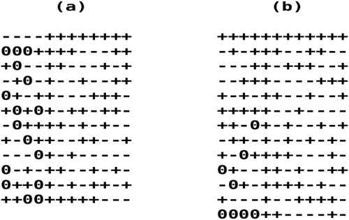
• 26-run ADSD: (0.925, 0.557, 0.409, 0, 0.084, 0.077) (see Figure 3 (b));

  Figure 3 Half fractions of (a) a 24-run MLFOD*(4) and (b) a 26-run ADSD for four 3-level factors and eight 2-level factors.

  

• 24-run MLFOD*(2): (0.926, 0.58, 0.2, 0, 0.183, 0.0);

• 24-run MLFOD*(3): (0.869, 0.603, 0.111, 0.111, 0.289, 0.0);

• 24-run MLFOD*(4): (0.852, 0.617, 0.125, 0.125, 0.204, 0.0) (see Figure 3 (a)).

This typical example, shows comparing to ADSDs, our MLFOD*s in general have higher d₂ but lower d₁ and lower r₁ but slightly higher r₂ and r₃.

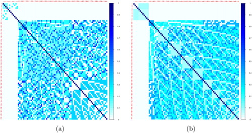
Figure 4 shows the correlation cell plots (CCPs) of our MLFOD*(4) and the ADSD whose half fractions are in Figure 3. These CCPs, advocated by Jones & Nachtsheim (2011), show the pairwise absolute correlation between the two terms under study as a colored square. Each plot in Figure 4 has 82 rows, 82 columns and 82² colored cells (82 = 4 + 12+${(}_{ 2}^{12})$). The color of each cell goes from white to dark. The white cells imply no correlation, while the dark ones a correlation of 1 or close to 1. It can be seen in Figure 4 that while the correlations among the 2-level MEs of our MLFOD* is zero, the correlation among the 3-level MEs of the ADSD is zero. This figure also shows that the magnitude of the correlation among the quadratic effects is more visible in the CCP of the ADSD than that of the MLFOD*.

Figure 4 Correlation Cell Plots of a 24-run MLFOD* and a 26-run ADSD for four 3-level factors and eight 2-level factors.

In this example, we assume four 3-level and seven 2-level factors, but factors E and J could be considered continuous. Below are the $(d_1,d_2,r_1,r_2,r_3,r_4)$ values of the three candidate designs for six 3-level factors and six 2-level factors:

• 26-run ADSD: (0.903, 0.452, 0.409, 0, 0.084, 0.077);

• 24-run MLFOD*(3): (0.808, 0.506, 0.111, 0.111, 0.289, 0.0);

• 24-run MLFOD*(4): (0.785, 0.516, 0.125, 0.125, 0.204, 0.0).

FOLDOVER could not find an MLFOD*(2) solution for this situation. The previous comment regarding the $d_1,d_2,r_1,r_2$ and r₃ values of these candidate designs applies.

Example 2: Irvine et al. (1996) described a $2^{13-9}$ pulping experiment investigating the best method to remove lignin during the pulping stage without negatively impacting the strength and yield. The 13 factors are: (A) Wood chip presoaked (yes/no); (B) Chips pre-steamed for 10 min at 110⁰C; (C) Initial effective alkali level in (6/12); (D) Sulfide level in impregnation in (3/10); (E) Liquor (black/white); (F) Liquor/wood ratio (3.5:1/6:1); (G) Impregnation temperature in ⁰C (110/150); (H) Impregnation pressure in kPa (190/1140); (J) Impregnation time in min (10/40); (K) Anthraquinone in (0.00/0.05); (L) Cook temperature in ⁰C (165/170); (M) Water quench (no/yes) and (N) Extended alkali wash for 1 hour (no/yes). This experiment was also reported in Mee (2009, p. 183). Again, like the previous experiment, we assume the experimenters are looking for the designs that treat the six factors C, D, G, H, J and K as 3-level quantitative factors instead of 2-level factors.

Below are the $(d_1,d_2,r_1,r_2,r_3,r_4)$ values of the four candidate designs for six 3-level factors and six 2-level factors:

• 30-run ADSD: (0.918, 0.455, 0.423, 0, 0.072, 0.067) (see Figure 5 (b));

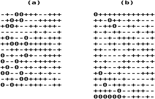
  Figure 5 Half fractions of (a) our 26-run MLFOD* and (b) 30-run ADSD for six 3-level factors and seven 2-level factors.

  

• 26-run MLFOD*(2): (0.899, 0.466, 0.182, 0.091, 0.084, 0.077);

• 26-run MLFOD*(3): (0.816, 0.511, 0.133, 0.2, 0.175, 0.077);

• 26-run MLFOD*(4): (0.827, 0.547, 0.083, 0.0, 0.092, 0.077) (see Figure 5 (a)).

In this rare example, our MLFOD*(4) was able to decrease r₁ without increasing r₂ or substantially increasing r₃.

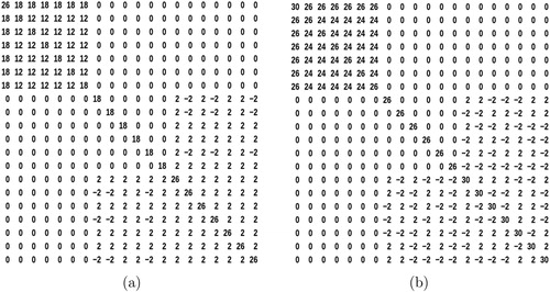
The CCPs of these two designs in Figure 5 are in Figure 6. It can be seen in Figures 4 and 6 that all MEs are orthogonal to the 2FIs. Also in these CCPs, the magnitude of the correlations among the quadratic effects of the candidate ADSDs are more severe than those of the MLFOD*s. At the same time, the magnitude of the correlations between the quadratic effects and the 2FIs of the candidate ADSDs is less visible than those of MLFOD*s. The ${\mathbf{X}}^{\prime }\mathbf{X}$ matrices of the two designs in this example are in Figure 7.

Figure 6 Correlation Cell Plots of (a) our 26-run MLFOD* and (b) 30-run ADSD for six 3-level factors and seven 2-level factors.

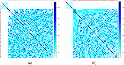
Figure 7 The X′X matrices of (a) our 26-run MLFOD* and (b) 30-run ADSD for six 3-level factors and seven 2-level factors.

In this second example, factors F and L could also be considered continuous. Below are the $(d_1,d_2,r_1,r_2,r_3,r_4)$ values of the two candidate designs for eight 3-level and five 2-level factors:

• 30-run ADSD: (0.905, 0.383, 0.423, 0, 0.072, 0.067);

• 26-run MLFOD(2): (0.875, 0.398, 0.409, 0.091, 0.084, 0.077);

• 26-run MLFOD(3): (0.788, 0.437, 0.133, 0.2, 0.175 0.077);

• 26-run MLFOD*(4): (0.743, 0.465, 0.083, 0.222, 0.277, 0.077).

Note that our 26-run MLFOD(2) and 26-run MLFOD(3) are not MLFOD*s. Like the previous example, comparing to ADSDs, our MLFOD*s in general have higher d₂ but lower d₁ and lower r₁ but slightly higher r₂ and r₃.

5 Conclusion

While most screening experiments include the 3-level quantitative factors, 2-level designs such as Plackett-Burman designs and FFDs of resolution III or IV have been used in practice. This paper introduces a new class of Hadamard matrix-based MLFODs. This class of design retains the core benefits of ADSDs, i.e., the orthogonality between the MEs and the 2FIs and the orthogonality between the MEs and the quadratic effects. In addition, it guarantees the orthogonality among 2-level columns when the input design is a Hadamard matrix or a Plackett-Burman design, has less severe correlation among the quadratic effects, requires fewer runs and is more flexible in the sense that the 3-level columns can include more mid-levels. The last feature is important considering the fact that experimenters often consider the mid-levels the desired ones and wish to replicate them more often. More importantly, at the end of the day, most users of MLFODs wish to collapse the MLFOD into a second-order one in a subset of significant factors. Clearly, the latter will be more D-efficient if the proportion of mid-levels in each of the 3-level factor of the design is reasonable.

Users using our MLFODs, however, should be aware that MLFOD*s are not always available when the number of 3-level factors exceeds the number of 2-level factors. Unlike ADSDs, MLFOD*s do not always guarantee the orthogonality among the 3-level factors. A referee has pointed out that DSDs (and MLFODs) are primarily screening designs which to some degree reflect the hierarchy principle and the most important effects are the main effects and not quadratic effects and interactions. In general an increase in the number of 0’s in each 3-level factors of an MLFOD will result in a design with higher d₂ but lower d₁ and lower r₁ but slightly higher r₂ and r₃. Therefore, it is mandatory that the experimenters have to take into account the requirement of the experiments and to look at the $(d_1,d_2,r_1,r_2,r_3,r_4)$ values of the candidate designs (which should also includes ADSDs) before choosing one.

The supplemental material contains 216 ADSDs, 205 MLFOD(2)s, 216 MLFOD($[\frac{m}{3}]$)s, 216 MLFOD($[\frac{m}{4}]$)s and 214 MLFOD($[\frac{m}{5}]$)s discussed in Section 4. Almost all MLFODs with $m_3<m_2$ are also MLFOD*s. Each ADSD or MLFOD includes the $(d_1,d_2,r_1,r_2,r_3,r_4)$ values and the half fraction in (1). Also included in the supplemental material are the file containing the pseudo-code of FOLDOVER, the java program hmld and the associated class files which implement the FOLDOVER algorithm in Section 3 and the input matrices we use to construct the MLFODs in this paper.

Acknowledgement

The authors would like to thank the editor, the associate editor and the two referees for their comments and suggestions which significantly improve the quality and readability of the paper. This research is funded by the Vietnam National University, Hanoi (VNU) under the project No. QG.18.03.

References

- Bullington, R.G., Lovin, S., Miller, D. M., & Woodall, W. H. (1993). Improvement of an Industrial Thermostat Using Designed Experiments. Journal of Quality Technology 25, 262-270.
- Draper, N.R. & Lin D.K.J. (1990) Small response surface designs. Technometrics 2, 187-194.
- Errore, A., Jones, B., Li B. & Nachtsheim, C. J. (2017) Benefits and Fast Construction of Eficient Two-Level Foldover Designs. Technometrics 59, 48-57.
- Hedayat, A. S & Wallis W. D. (1978) Hadamard Matrices and Their Applications The Annals of Statistics 6, 1184-1238.
- Irvine, G. M., Clark, N. B., & Recupero, C. (1996). Extended Delignifi- cation of Mature and Plantation Eucalypt Wood. 2. The effects of Chip Impregnation Factors. Appita Journal 49, 347-252.
- John, P.M.W. (1971), Statistical design and analysis of experiments, New York: McMillan.
- Jones, B., & Nachtsheim, C. J. (2011). A Class of Three Levels Designs for Definitive Screening in the Presence of Second-Order Effects, Journal of Quality Technology 43, 1-15.
- Jones, B., & Nachtsheim, C. J. (2013). Definitive Screening Designs with Added Two-Level Categorical Factors. Journal of Quality Technology 45, 121-129.
- Mee, R. W. (2009). A Comprehensive Guide to Factorial two-level Experimentation. New York, NY: Springer.
- Montgomery, D. C. (2017) Design and Analysis of Experiments, 9th Edition, John Wiley & Sons, Inc.
- Nachtsheim, A. C., Shen, W. & Lin, D. K, J. (2017), Two level Augmented Definitive Screening Designs, Journal of Quality Technology 49, 93-107.
- Nguyen, N. K. (1996) An Algorithmic Approach to Constructing Supersaturated Designs. Technometrics 1, 69-73.
- Nguyen, N. K. & Stylianou, S. (2013). Constructing Definitive Screening Designs Using Cyclic Generators, Journal of Statistics Theory & Practice 7, 713-724.
- Plackett, R.L. & Burman, J. P. (1946). The Design of Optimum Multifactorial Experiments. Biometrika 33, 305-25.
- Xiao, L. L; Lin, D. K. J. & Bai, F. S. (2012). Constructing Definitive Screening Designs Using Conference Matrices. Journal of Quality Technology 44, 2-8.