SPlit: An Optimal Method for Data Splitting

Abstract

In this article, we propose an optimal method referred to as SPlit for splitting a dataset into training and testing sets. SPlit is based on the method of support points (SP), which was initially developed for finding the optimal representative points of a continuous distribution. We adapt SP for subsampling from a dataset using a sequential nearest neighbor algorithm. We also extend SP to deal with categorical variables so that SPlit can be applied to both regression and classification problems. The implementation of SPlit on real datasets shows substantial improvement in the worst-case testing performance for several modeling methods compared to the commonly used random splitting procedure.

Keywords:

• Cross-validation
• Quasi-Monte Carlo
• Testing
• Training
• Validation

1 Introduction

For developing statistical and machine learning models, it is common to split the dataset into two parts: training and testing (Stone 1974; Hastie, Tibshirani, and Friedman 2009). The training part is used for fitting the model, that is, to estimate the unknown parameters in the model. The model is then evaluated for its accuracy using the testing dataset. The reason for doing this is because if we were to use the entire dataset for fitting, then the model would overfit the data and can lead to poor predictions in future scenarios. Therefore, holding out a portion of the dataset and testing the model for its performance before deploying it in the field can protect against unexpected issues that can arise due to overfitting.

In this article, we consider only datasets where each row is independent of other rows, that is, we will exclude cases such as time series data. The simplest and probably the most common strategy to split such a dataset is to randomly sample a fraction of the dataset. For example, 80% of the rows of the dataset can be randomly chosen for training and the remaining 20% can be used for testing. The aim of this article is to propose an optimal strategy to split the dataset.

Snee (1977) seemed to be the first one who has carefully investigated several data splitting strategies. He proposed DUPLEX as the best strategy which was originally developed by Kennard as an improvement to another popular strategy CADEX (Kennard and Stone 1969). Over the time, many other methods have been proposed in the literature for data splitting; see, for example, the survey in Reitermanová (2010) and the comparative study in Xu and Goodacre (2018). Some of these methods will be discussed in the next section after proposing a mathematical formulation of the problem.

It is also common to hold out a portion of the training set for validation. The validation set can be used for fine-tuning the model performance such as for choosing hyper-parameters or regularization parameters in the model. In fact, the training set can be divided into multiple sets and the model can be trained using cross-validation. Our proposed method for optimally splitting the dataset into training and testing can also be used for these purposes by applying the method repeatedly on the training set.

The article is organized as follows. In Section 2, we provide a mathematical formulation of the problem and propose an optimal splitting method called SPlit based on a technique for finding optimal representative points of a distribution known as support points (SP; Mak and Joseph 2018b). SP are defined only for continuous variables. Therefore, we extend the SP methodology to deal with categorical variables in Section 3 so that SPlit can be applied to both regression and classification problems. We apply SPlit on several real datasets in Section 4 and compare its performance with random subsampling. Some concluding remarks are given in Section 5.

2 Methodology

Let $\mathbf{X}=(X_1,\dots ,X_p)$ be the p input variables (or features) and Y the output variable. Let $\mathcal{D}={\{({\mathbf{X}}_i,Y_i)\}}_{i=1}^N$ be the dataset in hand. Our aim is to divide $\mathcal{D}$ into two disjoint and mutually exclusive sets: ${\mathcal{D}}^{\text{train}}$ and ${\mathcal{D}}^{\text{test}}$, where the training set ${\mathcal{D}}^{\text{train}}$ contains $N_{\text{train}}$ points and testing set ${\mathcal{D}}^{\text{test}}$ contains $N_{\text{test}}$ points with $N_{\text{train}}+N_{\text{test}}=N$.

2.1 Mathematical Formulation

Suppose the rows of the dataset are independent realizations from a distribution $F(\mathbf{X},Y)$:(1) $$({\mathbf{X}}_i,Y_i)\stackrel{\text{iid}}{\sim }F,i=1,\dots ,N.$$(1)

Let $g(\mathbf{X};\mathit{\theta })$ be the prediction model that we would like to fit to the data, where $\mathit{\theta }$ is a set of unknown parameters in the model. The unknown parameters $\mathit{\theta }$ will be estimated by minimizing a loss function $L(Y,g(\mathbf{X};\mathit{\theta }))$. Typical loss functions include squared or absolute error loss. More generally, the negative of the log-likelihood can be used as a loss function.

In postulating a prediction model $g(\mathbf{X};\mathit{\theta })$, our hope is that it will be close to the true model $E(Y|\mathbf{X})$ for some value of $\mathit{\theta }$. However, the postulated model could be wrong and there may not exist a true value for $\mathit{\theta }$. Thus, it makes sense to try out different possible models on a training set and check their performance on the testing set so that we can identify the model that is closer to the truth.

The unknown parameters $\mathit{\theta }$ can be estimated from the training set as follows:(2) $$\widehat{\mathit{\theta }}=\underset{\mathit{\theta }}{\text{Argmin}}\frac{1}{N_{\text{train}}}\sum _{i=1}^{N_{\text{train}}}L(Y_i^{\text{train}},g({\mathbf{X}}_i^{\text{train}};\mathit{\theta })),$$(2) which is a valid estimator provided that(3) $$({\mathbf{X}}_i^{\text{train}},Y_i^{\text{train}})\sim F,\hspace{1em}i=1,\dots ,N_{\text{train}}.$$(3)

How should we split the dataset to obtain training and testing sets? We propose that the dataset should be split in such a way that the testing set gives an unbiased and efficient evaluation of the model’s performance fitted using the training set.

To quantify the model’s performance, define the generalization error as in (Hastie, Tibshirani, and Friedman 2009, chap. 7) by(4) $$\mathcal{E}=E_{\mathbf{X},Y}\{L(Y,g(\mathbf{X};\widehat{\mathit{\theta }}))|{\mathcal{D}}^{\text{train}}\},$$(4) where the expectation is taken with respect to a realization $(\mathbf{X},Y)$ from F. Note that we do not include the randomness in $\widehat{\mathit{\theta }}$ induced by ${\mathcal{D}}^{\text{train}}$ for computing the expectation.

We can estimate $\mathcal{E}$ if we have a sample of observations from F that is independent of the training set. We can use the testing set for this purpose. Thus, an estimate of $\mathcal{E}$ can be obtained as(5) $$\widehat{\mathcal{E}}=\frac{1}{N_{\text{test}}}\sum _{i=1}^{N_{\text{test}}}L(Y_i^{\text{test}},g({\mathbf{X}}_i^{\text{test}};\widehat{\mathit{\theta }})),$$(5) which works if(6) $$({\mathbf{X}}_i^{\text{test}},Y_i^{\text{test}})\sim F,\hspace{1em}i=1,\dots ,N_{\text{test}}.$$(6)

A simple way to ensure condition (6) is to randomly sample $N_{\text{test}}$ points from $\mathcal{D}$. Then, Equation (5)(5) $$\widehat{\mathcal{E}}=\frac{1}{N_{\text{test}}}\sum _{i=1}^{N_{\text{test}}}L(Y_i^{\text{test}},g({\mathbf{X}}_i^{\text{test}};\widehat{\mathit{\theta }})),$$(5) can be viewed as the Monte Carlo (MC) estimate of $\mathcal{E}$. The question we are trying to answer is, if there is a better way to sample from $\mathcal{D}$ so that we can get a more efficient estimate of $\mathcal{E}$. The answer to this question is affirmative. We can use quasi-Monte Carlo (QMC) methods to improve the estimation of $\mathcal{E}$. It is well known that the error of MC estimates decreases at the rate $\mathcal{O}(1/\sqrt{N_{\text{test}}})$, whereas when sampling from uniform distributions, the QMC error rate can be shown to be almost $\mathcal{O}(1/N_{\text{test}})$ (Niederreiter 1992). This is a substantial improvement in the error rate. However, most QMC methods focus on uniform distributions (Owen 2013). Recently, Mak and Joseph (2018b) developed a method known as SP to obtain a QMC sample from general distributions. Although their theoretical results guarantee a convergence rate faster than MC by only a $\text{log}\hspace{0.17em}{N}_{\text{test}}$ factor, much faster convergence rates are observed in practical implementations. This leads us to the proposed method SPlit (stands for SP-based split). We will discuss the method of SP and SPlit in detail after reviewing the existing data splitting methods in the next section.

2.2 Review of Data Splitting Methods

Interestingly, the original motivation behind CADEX (Kennard and Stone 1969) and DUPLEX (Snee 1977) was to create two sets with similar statistical properties, which agrees with the distributional condition mentioned in Equation (6)(6) $$({\mathbf{X}}_i^{\text{test}},Y_i^{\text{test}})\sim F,\hspace{1em}i=1,\dots ,N_{\text{test}}.$$(6) . However, these algorithms cannot achieve this objective. For example, consider a two-dimensional data generated using $(X_{1i},X_{2i})\stackrel{\text{iid}}{\sim }{N}_2(\mathbf{0},\mathbf{\Sigma })$ for $\mathrm{(}\text{HTML}\mathrm{ }\text{translation}\mathrm{ }\text{failed}\mathrm{)}$, where $\mathbf{0}=(0,0)\prime$ and ${\Sigma }_{jk}={.5}^{|j-k|}$. We will omit the response here because these algorithms do not use it. Let N = 1000 and $N_{\text{test}}=100$. 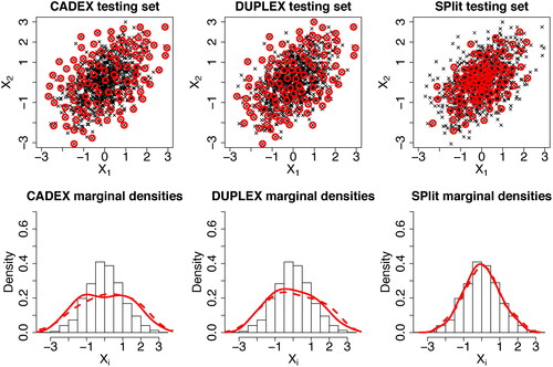The CADEX and DUPLEX testing sets obtained using the R package prospectr (Stevens and Ramirez-Lopez 2020) are shown in the left and middle top panels of Figure 1. We can see that both CADEX and DUPLEX testing points are too spread out and therefore, their distributions do not match with the distribution of the data. This can be seen more clearly in the marginal distributions shown in the bottom panels. For comparison, the testing set generated using the proposed SPlit method is shown in the top-right panel. We can see that its distribution matches quite well with the distribution of the full data, as desired.

Fig. 1 Comparison of CADEX and DUPLEX testing sets with SPlit testing set. Hundred testing points (red circles) are chosen from 1000 data points (black crosses). In the lower panels, the marginal densities of the testing sets are plotted over the histogram of the full data.

The sample set partitioning based on joint X–Y distances (SPXY) algorithm (Galvão et al. 2005) is a modification of the CADEX algorithm which incorporates the distances computed from the response values. Although incorporating Y was in the right direction of Equation (6)(6) $$({\mathbf{X}}_i^{\text{test}},Y_i^{\text{test}})\sim F,\hspace{1em}i=1,\dots ,N_{\text{test}}.$$(6) , the algorithm suffers from the same issues of CADEX and DUPLEX algorithms. Bowden, Maier, and Dandy (2002) proposed a data splitting method which uses global optimization techniques to match the mean and standard deviations of the testing set and the full data. This is again in the right direction of Equation (6)(6) $$({\mathbf{X}}_i^{\text{test}},Y_i^{\text{test}})\sim F,\hspace{1em}i=1,\dots ,N_{\text{test}}.$$(6) , however, matching the first two moments does not ensure distributional matching. May, Maier, and Dandy (2010) proposed further improvement to the foregoing methodology using clustering-based stratified sampling. Although this provides an improvement, it is well known that clustering distorts the original distribution (Zador 1982) and hence cannot satisfy Equation (6)(6) $$({\mathbf{X}}_i^{\text{test}},Y_i^{\text{test}})\sim F,\hspace{1em}i=1,\dots ,N_{\text{test}}.$$(6) . In summary, none of existing data splitting methods except the random subsampling can ensure the distributional condition given in either Equation (6)(6) $$({\mathbf{X}}_i^{\text{test}},Y_i^{\text{test}})\sim F,\hspace{1em}i=1,\dots ,N_{\text{test}}.$$(6) or Equation (3)(3) $$({\mathbf{X}}_i^{\text{train}},Y_i^{\text{train}})\sim F,\hspace{1em}i=1,\dots ,N_{\text{train}}.$$(3) .

Before proceeding further, we would like to mention about another possible approach to solve the problem. One could think about splitting the dataset in such a way that the training set gives the best possible estimation of the model under a given loss function. For example, it is well known that the best estimate of a linear regression model with linear effects of the predictors under the least-square criterion can be obtained by choosing the extreme values of the data from the predictor-space (Wang, Yang, and Stufken 2019). Although such a choice can minimize the variance of the parameter estimates, the model may not perform well in the testing set if the original dataset is not generated from such a linear model. In our opinion, the testing set should provide a set of samples for an unbiased evaluation of the model performance and detect possible model deviations. For example, if we detect that quadratic terms are needed in the linear regression model, then having a training dataset with only extreme values of the predictors is not going to be useful. Therefore, the splitting method should be independent of the modeling choice and the loss function. Random subsampling achieves this aim and we will show that SP will achieve it even better!

Although SP have been used in the past for subsampling from big data (Mak and Joseph 2018a), it was done for the purpose of saving storage space and time for fitting computationally expensive models due to limited resources. On the other hand, data reduction is not the objective in our problem. After assessing the model’s performance using the testing set, the model will be re-estimated using the full data before deploying it for future predictions.

2.3 Support Points

Let $F(Z)$ and the empirical distribution of a set of points $z_1,\dots ,z_n$ is defined as (Székely and Rizzo 2013)(7) $$ED=\frac{2}{n}{\displaystyle \sum _{i=1}^n\mathbb{E}}\left|\right|z_i-Z|{|}_2-\frac{1}{n^2}{\displaystyle \sum _{i=1}^n{\displaystyle \sum _{j=1}^n|}}|z_i-z_j|{|}_2-\mathbb{E}||Z-Z\prime |{|}_2,$$(7) where $Z,Z\prime ~F,\left|\right|·|{|}_2$ is the Euclidean distance, and the expectations are taken with respect to F. Note that for the Euclidean distance to make sense, all the variables are standardized to have zero mean and unit variance. The energy distance will be small if the empirical distribution of $z_1,\dots ,z_n$ is close to F. Therefore, Mak and Joseph (2018b) defined the SP of F as the minimizer of the energy distance:(8) $$\begin{array}{l}{\left\{z_i^{*}\right\}}_{i=1}^n\in \underset{z_1,\dots ,z_n}{\text{Argmin}}ED=\underset{z_1,\dots ,z_n}{\text{Argmin}}\{\frac{2}{n}{\displaystyle \sum _{i=1}^n\mathbb{E}}\left|\right|z_i-Z|{|}_2\\ -\frac{1}{n^2}{\displaystyle \sum _{i=1}^n{\displaystyle \sum _{j=1}^n|}}|z_i-z_j|{|}_2\}.\end{array}$$(8)

They can be viewed as the representative points of the distribution F, which is the best set of n points to represent F according to the energy distance criterion. Mak and Joseph (2018b) showed that SP converge in distribution to F and therefore, they can be viewed as a QMC sample from F. This property makes SP different from other representative points of a distribution such as MSE-rep points (Fang and Wang 1994) or principal points (Flury 1990) which do not possess distributional convergence (Zador 1982).

In our problem, we do not have F. Instead we only have a dataset $\mathcal{D}$, which is a set of independent realizations from F. Therefore, to compute the SP, we can replace the expectation in Equation (8)(8) $$\begin{array}{l}{\left\{z_i^{*}\right\}}_{i=1}^n\in \underset{z_1,\dots ,z_n}{\text{Argmin}}ED=\underset{z_1,\dots ,z_n}{\text{Argmin}}\{\frac{2}{n}{\displaystyle \sum _{i=1}^n\mathbb{E}}\left|\right|z_i-Z|{|}_2\\ -\frac{1}{n^2}{\displaystyle \sum _{i=1}^n{\displaystyle \sum _{j=1}^n|}}|z_i-z_j|{|}_2\}.\end{array}$$(8) with a Monte Carlo average computed over $\mathcal{D}$:(9) $$\begin{array}{l}{\left\{z_i^{*}\right\}}_{i=1}^n\in \underset{z_1,\cdots ,z_n}{\text{Argmin}}\{\frac{2}{nN}{\displaystyle \sum _{i=1}^n{\displaystyle \sum _{j=1}^N|}}|z_i-Z_j|{|}_2\\ -\frac{1}{n^2}{\displaystyle \sum _{i=1}^n{\displaystyle \sum _{j=1}^n|}}|z_i-z_j|{|}_2\}.\end{array}$$(9)

This simple extension to real data settings is another advantage of SP, which cannot be done for other representative points such as minimum energy design (Joseph et al. 2015) and Stein points (Chen et al. 2018) even though they possess distributional convergence.

At first sight, the optimization in Equation (9)(9) $$\begin{array}{l}{\left\{z_i^{*}\right\}}_{i=1}^n\in \underset{z_1,\cdots ,z_n}{\text{Argmin}}\{\frac{2}{nN}{\displaystyle \sum _{i=1}^n{\displaystyle \sum _{j=1}^N|}}|z_i-Z_j|{|}_2\\ -\frac{1}{n^2}{\displaystyle \sum _{i=1}^n{\displaystyle \sum _{j=1}^n|}}|z_i-z_j|{|}_2\}.\end{array}$$(9) appears to be a very hard problem. The objective function is nonlinear and nonconvex. Moreover, the number of variables in the optimization is $n(p+1)$, which can be extremely high even for small datasets. However, the objective function has a nice feature; it is a difference of two convex functions. By exploiting this feature, Mak and Joseph (2018b) developed an efficient algorithm based on difference-of-convex programming techniques, which can be used for quickly finding the SP. Although a global optimum is not guaranteed, an approximate solution can be obtained in a reasonable amount of time. Their algorithm is implemented in the R package support (Mak 2019). Although it is possible to create representative points using other goodness-of-fit test statistics (Hickernell 1999) and kernel functions (Chen, Welling, and Smola 2010) instead of the energy distance criterion, they do not seem to possess the computational advantage and robustness of SP.

2.4 SPlit

We can use the SP obtained from Equation (9)(9) $$\begin{array}{l}{\left\{z_i^{*}\right\}}_{i=1}^n\in \underset{z_1,\cdots ,z_n}{\text{Argmin}}\{\frac{2}{nN}{\displaystyle \sum _{i=1}^n{\displaystyle \sum _{j=1}^N|}}|z_i-Z_j|{|}_2\\ -\frac{1}{n^2}{\displaystyle \sum _{i=1}^n{\displaystyle \sum _{j=1}^n|}}|z_i-z_j|{|}_2\}.\end{array}$$(9) as the testing set with $n=N_{\text{test}}$ and the remaining data can be used as the training set. Alternatively, we can use SP to obtain the training set with $n=N_{\text{train}}$ and then use the remaining data as the testing set. However, the computational complexity of the algorithm used for generating SP is $\mathcal{O}(n^2(p+1))$. Since $N_{\text{test}}$ is usually smaller than $N_{\text{train}}$, it will be faster to generate the testing set using SP than the training set. In general, we let $n=\text{min}\{N_{\text{test}},N_{\text{train}}\}=\text{min}\{N\gamma ,N(1-\gamma )\}$, where $\gamma =N_{\text{test}}/N$ is the splitting ratio.

As discussed earlier, the testing set generated using SP is expected to work better than a random sample from $\mathrm{(}\text{HTML}\mathrm{ }\text{translation}\mathrm{ }\text{failed}\mathrm{)}$. However, there is one drawback. Support points need not be a subsample of the original dataset. This is because the optimization in Equation (9)(9) $$\begin{array}{l}{\left\{z_i^{*}\right\}}_{i=1}^n\in \underset{z_1,\cdots ,z_n}{\text{Argmin}}\{\frac{2}{nN}{\displaystyle \sum _{i=1}^n{\displaystyle \sum _{j=1}^N|}}|z_i-Z_j|{|}_2\\ -\frac{1}{n^2}{\displaystyle \sum _{i=1}^n{\displaystyle \sum _{j=1}^n|}}|z_i-z_j|{|}_2\}.\end{array}$$(9) is done on a continuous space and therefore, the optimal solution need not be part of $\mathcal{D}$. To get a subsample, we actually need to solve the following discrete optimization problem:(10) $$\begin{array}{c}{\left\{{\mathbf{z}}_i^{*}\right\}}_{i=1}^n\in \underset{{\mathbf{z}}_1,\dots ,{\mathbf{z}}_n\in \mathcal{D}}{\text{Argmin}}\{\frac{2}{nN}\sum _{i=1}^n\sum _{j=1}^N||{\mathbf{z}}_i-{\mathbf{Z}}_j|{|}_2\\ -\frac{1}{n^2}\sum _{i=1}^n\sum _{j=1}^n||{\mathbf{z}}_i-{\mathbf{z}}_j|{|}_2\frac{2}{nN}\sum _{i=1}^n\}.\end{array}$$(10)

Our initial attempts to solve this problem using state-of-the-art integer programming techniques showed that they are accurate, but too slow in finding the optimal solution. Computational speed is crucial for our method to succeed because otherwise it will not be attractive against the computationally cheap alternative of random subsampling. Therefore, here we propose an approximate but efficient algorithm to subsample from $\mathcal{D}$.

Algorithm 1 SPlit: Splitting a dataset $\mathcal{D}$ with splitting ratio γ [R package: SPlit]

1: Input $\mathcal{D}\in {\mathbb{R}}^{N\times (p+1)}$ and $\gamma =N_{\text{test}}/N$

2: Standardize the columns of $\mathcal{D}$

3: $n\leftarrow \text{min}\{N\gamma ,N(1-\gamma )\}$

4: Compute ${\left\{{\mathbf{z}}_i^{*}\right\}}_{i=1}^n$ using (9)

5:${\mathcal{D}}_1\leftarrow \left\{\right\}$

6:for $i\in \{1,\dots ,n\}$ do

7:$\widehat{\mathbf{u}}\in {\text{argmin}}_{\mathbf{u}}\left\{\right||\mathbf{u}-{\mathbf{z}}_i^{*}|{|}_2:\mathbf{u}\in \mathcal{D}\}$

8:${\mathcal{D}}_1\leftarrow {\mathcal{D}}_1\cup \left\{\widehat{\mathbf{u}}\right\}$

9:$\mathcal{D}\leftarrow \mathcal{D}\setminus \left\{\widehat{\mathbf{u}}\right\}$

10:end for

11:${\mathcal{D}}_2\leftarrow \mathcal{D}$

12:return ${\mathcal{D}}_1,{\mathcal{D}}_2$

We will first find the SP in a continuous space as in Equation (9)(9) $$\begin{array}{l}{\left\{z_i^{*}\right\}}_{i=1}^n\in \underset{z_1,\cdots ,z_n}{\text{Argmin}}\{\frac{2}{nN}{\displaystyle \sum _{i=1}^n{\displaystyle \sum _{j=1}^N|}}|z_i-Z_j|{|}_2\\ -\frac{1}{n^2}{\displaystyle \sum _{i=1}^n{\displaystyle \sum _{j=1}^n|}}|z_i-z_j|{|}_2\}.\end{array}$$(9) , which is very fast. We will then choose the closest points in $\mathcal{D}$ to ${\left\{{\mathbf{z}}_i^{*}\right\}}_{i=1}^n$ according to the Euclidean distance. This can be done efficiently even for big datasets using KD-Tree based nearest neighbor algorithms. However, a naive nearest neighbor assignment can lead to duplicates and therefore, the remaining data points can become more than N – n. Moreover, separating the points can increase the second term in Equation (10)(10) $$\begin{array}{c}{\left\{{\mathbf{z}}_i^{*}\right\}}_{i=1}^n\in \underset{{\mathbf{z}}_1,\dots ,{\mathbf{z}}_n\in \mathcal{D}}{\text{Argmin}}\{\frac{2}{nN}\sum _{i=1}^n\sum _{j=1}^N||{\mathbf{z}}_i-{\mathbf{Z}}_j|{|}_2\\ -\frac{1}{n^2}\sum _{i=1}^n\sum _{j=1}^n||{\mathbf{z}}_i-{\mathbf{z}}_j|{|}_2\frac{2}{nN}\sum _{i=1}^n\}.\end{array}$$(10) and thus potentially improve the energy distance criterion. This can be achieved by doing the nearest neighbor assignment sequentially. Our method is summarized in Algorithm 1 and is implemented in the R package SPlit. A critical step in this algorithm is to update the KD-Tree efficiently when a point is removed from the dataset. We use nanoflann, a C++ header-only library (Blanco and Rai 2014), which allows for lazy deletion of a data point from the KD-Tree without having to rebuild the KD-Tree every time a point is removed from the dataset.

2.5 Visualization

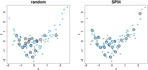
Consider a simple example for visualization purposes. Suppose we generate N = 100 points as follows: $X_i\stackrel{\text{iid}}{\sim }N(0,1)$ and $Y_i|X_i\stackrel{\text{iid}}{\sim }N(X_i^2,1)$ for $i=1,\dots ,N$. Both X and Y values are standardized to have zero mean and unit variance. Figure 2 shows the optimal testing set obtained using SPlit and a random testing set obtained using random subsampling without replacement. We can see that the points in the SPlit testing set are well spread out throughout the region and provide a much better point set to evaluate the model performance than the random testing set.

Fig. 2 The circles are the testing set obtained using random (left) and SPlit (right) subsampling.

Most statistical and machine learning models have some hyper parameters or regularization parameters, which are commonly estimated from the training set by holding out a validation set, say of size $N_{\text{valid}}$. One simple approach to create an optimal validation set is to apply the SPlit algorithm on the training set. However, it may happen that such a set is close to the points in the testing set, which is not good as it may lead to a biased testing performance. We want the validation points to stay away from the testing points so that the testing performance is not influenced by the model estimation/validation step. This can be achieved as follows. Let $\{{\mathbf{z}}_1,\dots ,{\mathbf{z}}_{N_{\text{test}}}\}$ be the testing set and $\{{\mathbf{z}}_{N_{\text{test}}+1},\dots ,{\mathbf{z}}_n\}$ the validation set, where $n=N_{\text{test}}+N_{\text{valid}}$. Then, the optimal validation points can be obtained as(11) $$\begin{array}{c}{\left\{{\mathbf{z}}_i^{*}\right\}}_{i=N_{\text{test}}+1}^n\in \underset{{\mathbf{z}}_{N_{\text{test}}+1},\dots ,{\mathbf{z}}_n\in \mathcal{D}}{\text{Argmin}}\{\frac{2}{nN}\sum _{i=1}^n\sum _{j=1}^N||{\mathbf{z}}_i-{\mathbf{Z}}_j|{|}_2\\ -\frac{1}{n^2}\sum _{i=1}^n\sum _{j=1}^n||{\mathbf{z}}_i-{\mathbf{z}}_j|{|}_2\},\\ \end{array}$$(11) where the optimization takes place only over the validation points with the testing points fixed at $\{{\mathbf{z}}_1^{*},\dots ,{\mathbf{z}}_{N_{\text{test}}}^{*}\}$. Because of the second term in the energy distance criterion, the validation points will move away from the testing points.

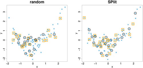
Figure 3 shows 20 points selected out of the 80 training points using Equation (11)(11) $$\begin{array}{c}{\left\{{\mathbf{z}}_i^{*}\right\}}_{i=N_{\text{test}}+1}^n\in \underset{{\mathbf{z}}_{N_{\text{test}}+1},\dots ,{\mathbf{z}}_n\in \mathcal{D}}{\text{Argmin}}\{\frac{2}{nN}\sum _{i=1}^n\sum _{j=1}^N||{\mathbf{z}}_i-{\mathbf{Z}}_j|{|}_2\\ -\frac{1}{n^2}\sum _{i=1}^n\sum _{j=1}^n||{\mathbf{z}}_i-{\mathbf{z}}_j|{|}_2\},\\ \end{array}$$(11) . A random subsample is also shown in the same figure for comparison. Clearly, the optimal validation set created using our method is a much better representative set of the original dataset and therefore, it can do a much better job in tuning the hyper-parameter or regularization parameter than using a random validation set. In fact, we can sequentially divide the training set into K sets by repeated application of this method and use them for K-fold cross-validation. Because of the importance of this problem, we will leave this topic for future research.

Fig. 3 The squares are the validation set obtained using random (left) and SPlit (right) subsampling from the training set. The testing set is shown as circles.

2.6 Simulations

Since SP create a dependent set, one may wonder if the testing set and training set are related and if the dependence will create a bias in the estimation of the generalization error in Equation (5)(5) $$\widehat{\mathcal{E}}=\frac{1}{N_{\text{test}}}\sum _{i=1}^{N_{\text{test}}}L(Y_i^{\text{test}},g({\mathbf{X}}_i^{\text{test}};\widehat{\mathit{\theta }})),$$(5) . We will perform some simulations to check this. Consider again the data-generating model discussed in the previous section(12) $$Y_i=X_i^2+{ϵ}_i,$$(12) where ${ϵ}_i\stackrel{\text{iid}}{\sim }N(0,1)$ and $X_i\stackrel{\text{iid}}{\sim }N(0,1)$, for $i=1,\dots ,N$. Let N = 1000. Suppose we fit the following rth degree polynomial model to the data:$$Y_i=g(X_i;\mathit{\theta })+{ϵ}_i,$$ where $g(X;\mathit{\theta })={\theta }_0+{\theta }_{1}X+{\theta }_2{X}^2+\cdots +{\theta }_r{X}^r$ and ${ϵ}_i\stackrel{\text{iid}}{\sim }N(0,{\sigma }^2)$. The unknown parameters $\mathit{\theta }=({\theta }_0,{\theta }_1,\dots ,{\theta }_r)\prime$ can be estimated from the training set using least squares. The generalization error can then be computed as follows:$$\begin{array}{c}\mathcal{E}=E_{X,Y}\left[{\{Y-g(X;\widehat{\theta })\}}^2|{\mathcal{D}}^{\text{train}}\right]\\ =E_{X,Y}\left[{\{Y-g(X;\widehat{\theta })\}}^2\right]\hspace{1em}\mathrm{(}\text{by}\mathrm{ }\text{independence}\mathrm{)}\\ =E_X\left(E_{Y|X}\left[{\{Y-g(X;\widehat{\theta })\}}^2|X\right]\right)\\ =E_X\left({\{X^2-g(X;\widehat{\mathit{\theta }})\}}^2\right)+1.\end{array}$$

We can divide a given dataset into training and testing sets using various data splitting methods and estimate the generalization error using Equation (5)(5) $$\widehat{\mathcal{E}}=\frac{1}{N_{\text{test}}}\sum _{i=1}^{N_{\text{test}}}L(Y_i^{\text{test}},g({\mathbf{X}}_i^{\text{test}};\widehat{\mathit{\theta }})),$$(5) . Thus, we can compute the estimation error of a data splitting method as $\widehat{\mathcal{E}}-\mathcal{E}$. For comparison, we use SPlit, random subsampling, CADEX, and DUPLEX. This procedure is repeated 100 times by generating testing sets with splitting ratios of 10% and 50%. Owing to the deterministic nature, CADEX and DUPLEX produce the same testing set each time. On the other hand, some variability is observed in the testing sets produced by SPlit, which is mainly due to the random initialization and convergence to local optima of the SP’ algorithm. Figure 4 shows the estimation errors over different values of r.

Fig. 4 The error in the estimation of generalization error with splitting ratios of 10% (left) and 50% (right) for different data splitting methods over 100 iterations.

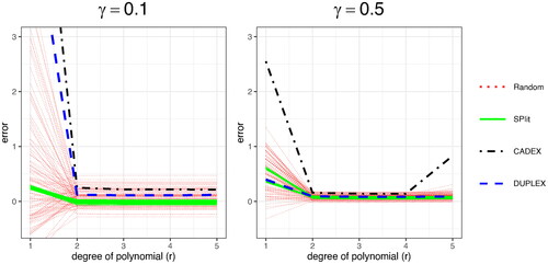
We can see that the bias in the estimation of generalization error using SPlit is small compared to the other data splitting methods. This confirms the validity of the proposed method.

3 Categorical Variables

Energy distance in Equation (7)(7) $$ED=\frac{2}{n}{\displaystyle \sum _{i=1}^n\mathbb{E}}\left|\right|z_i-Z|{|}_2-\frac{1}{n^2}{\displaystyle \sum _{i=1}^n{\displaystyle \sum _{j=1}^n|}}|z_i-z_j|{|}_2-\mathbb{E}||Z-Z\prime |{|}_2,$$(7) is defined only for continuous variables because its definition involves Euclidean distances and therefore, SP can only be found for datasets with continuous variables. However, a dataset can have categorical predictors and/or responses. Therefore, it is important to extend the SP methodology to deal with categorical variables in order to implement SPlit.

For simplicity of notations, let us consider the case of only a single categorical variable, which could be a predictor or a response. It is easy to extend our methodology to multiple categorical variables, which will be explained later. Let m be the number of levels of the categorical variable and N_i be the corresponding number of points in the dataset at the ith level, $i=1,\dots ,m$.

The most naive approach to deal with a categorical variable is to simply ignore it and find the n SP from a dataset containing N points using only the continuous variables as in Equation (9)(9) $$\begin{array}{l}{\left\{z_i^{*}\right\}}_{i=1}^n\in \underset{z_1,\cdots ,z_n}{\text{Argmin}}\{\frac{2}{nN}{\displaystyle \sum _{i=1}^n{\displaystyle \sum _{j=1}^N|}}|z_i-Z_j|{|}_2\\ -\frac{1}{n^2}{\displaystyle \sum _{i=1}^n{\displaystyle \sum _{j=1}^n|}}|z_i-z_j|{|}_2\}.\end{array}$$(9) . For illustration, consider the same example used in Section 2.4, except that we generate the data as follows. Let $X_{1i}\stackrel{\text{iid}}{\sim }N(0,1)$ and $X_{2i}|X_{1i}\stackrel{\text{iid}}{\sim }N(X_{1i}^2,1)$ for $i=1,\dots ,N$ with N = 100. They are scaled to have zero mean and unit variance. Consider a nominal categorical response variable with three levels: Red, Green, and Blue. The points are classified as Red with probability $\Phi (-6X_1-X_2-5)$ and Blue with probability $\Phi (6X_1-X_2-5)$, where $\Phi (·)$ is the standard normal distribution function. The remaining points are classified as Green. The data are shown in Figure 5.

Fig. 5 The circles are the testing set obtained using naive method (left), stratified proportional method (center), and the proposed coding-based method (right). The three categorical levels are shown as red triangles, green pluses, and blue crosses.

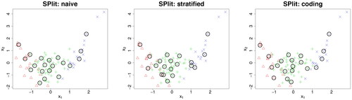
Suppose our aim is to generate a testing set of 20 points. The result of applying the naive method is shown in the left panel of Figure 5. In this dataset, there are $N_1=21$ Red, $N_2=59$ Green, and $N_3=20$ Blue. A testing set gives a good representation of the categorical variable if(13) $$\frac{n_i}{n}\approx \frac{N_i}{N}\text{forall}i=1,\dots ,m,$$(13) where n_i is the number of testing samples for the ith level. Thus, we should have approximately four Red, 12 Green, and four Blue in the testing set. However, the naive method gives only two Red and three Blue, which is quite disproportionate to the number of Red and Blue in the dataset. This is expected because the naive method does not use the information in the categorical response for splitting.

Another possible approach that can ensure the proportional sampling in Equation (13)(13) $$\frac{n_i}{n}\approx \frac{N_i}{N}\text{forall}i=1,\dots ,m,$$(13) is to first choose $n_i\approx N_i/Nn$ and then find n_i SP from the dataset containing only the ith level of the categorical variable while ignoring the remaining part of the dataset. The results of this stratified proportional method is shown in the middle panel of Figure 5. We can see that some points are too close and almost overlapping. Thus, although the stratified proportional sampling approach ensures perfect balancing of categorical levels, the SP in the continuous space may not be representative.

A yet another approach to deal with categorical variables is to first convert them into numerical variables and then use the methodology that we developed earlier for continuous variables. The first step is to represent the m levels of the categorical variable using m – 1 dummy variables assuming that the model has a parameter to represent the mean of the data. There are many choices for creating the dummy variables such as treatment coding, Helmert coding, sum coding, orthogonal polynomial coding, etc. (Faraway 2015, chap.14). Here we use Helmert coding as we have observed better numerical stability with it in the SP’ algorithm.

Consider the example again. Using Helmert coding, the Red, Green, and Blue levels are represented using two dummy variables $d_1=(-1,1,0)$ and $d_2=(-1,-1,2)$. Now the SPlit algorithm can be applied after standardizing the four columns of the augmented dataset. The result is shown in the last panel of Figure 5. We can see that the categorical levels are well-balanced and the points are well-spread out in the continuous space. Thus, this coding approach seems to work very well. Moreover, it can be easily adapted for ordinal categorical variables through scoring (Wu and Hamada 2011, p. 647). Furthermore, it can be used for multiple categorical variables by coding each variable separately. Thus, this approach appears to be very general and simple to implement and therefore, we will adopt it in the SPlit algorithm to handle categorical variables.

4 Examples

In this section, we will compare SPlit with random subsampling on real datasets for both regression and classification problems.

4.1 Regression

Consider the concrete compressive strength dataset from Yeh (1998) which can be obtained from the UCI Machine Learning Repository (Dua and Graff 2017). This dataset has eight continuous predictors pertaining to the concrete’s ingredients and age. The response is the concrete’s compressive strength. We will make an 80-20 split of this dataset which has 1, 030 rows. Thus $N_{\text{train}}=824$ and $N_{\text{test}}=206$. The split is done using both SPlit and random subsampling. All the nine variables are normalized to mean 0 and standard deviation 1 before splitting.

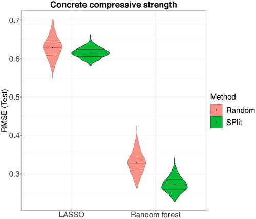
A good splitting procedure should work well for all possible modeling choices. Therefore, to check the robustness against different modeling choices, we choose a linear regression model with linear main effects estimated using LASSO (Tibshirani 1996) and a nonlinear-nonparametric regression model estimated using random forest (Breiman 2001). Both the models are fitted on the training set using the default settings of the R packages glmnet (Friedman, Hastie, and Tibshirani 2010) and randomForest (Liaw and Wiener 2002). Then we compute the root-mean-squared prediction error (RMSE) on the testing set to evaluate the models’ prediction performance. We repeat this procedure 500 times, where the same split is used for fitting both the LASSO and random forest.

The testing RMSE values for the 500 simulations are shown in Figure 6. We can see that on the average the testing RMSE is lower for SPlit compared to random subsampling. This improvement is much larger for random forest compared to LASSO. We also note significant improvement in the worst-case performance of SPlit over random subsampling. Furthermore, the variability in the testing RMSE is much smaller for SPlit compared to random subsampling and therefore, a more consistent conclusion can be drawn using SPlit. Thus, the simulation clearly shows that SPlit produces testing and training set that are much better for model fitting and evaluation. Computation of SPlit for this dataset took on an average 1.6 seconds on a computer with 6-core 2.6 GHz Intel processor, which is a negligibly small price that we need to pay for the improved performance over random subsampling.

Fig. 6 Distribution of RMSE over 500 random and SPlit subsampling splits for the concrete compressive strength dataset.

We repeated the simulation with several other datasets, namely Abalone (Nash et al. 1994), Airfoil self-noise (Brooks, Pope, and Marcolini 1989), Meat spectroscopy (Thodberg 1993), and Philadelphia birthweights (Elo, Rodriguez, and Lee 2001). Abalone and Airfoil self-noise datasets can be obtained from the UCI machine learning repository (Dua and Graff 2017), while Meat spectorscopy and Philadelphia birthweights can be obtained from the faraway (Faraway 2015) package in R. The details of these datasets are summarized in Table 1. Figure 7 shows the testing RMSE values for both LASSO and random forest. We see similar trends as before on all the datasets; SPlit gives a better testing performance on the average than random subsampling and a substantial improvement in the worst-case testing performance.

Fig. 7 Distribution of RMSE over 500 random and SPlit subsampling splits for the datasets described in Table 1.

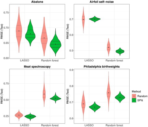
Table 1 Description of datasets considered for regression.

Dataset	Size	Predictors	Response
Abalone	4177 × 9	7 Continuous 1 categorical (3 levels)	Continuous
Airfoil self-noise	1503 × 6	5 Continuous	Continuous
Meat spectroscopy	215 × 101	100 Continuous	Continuous
Philadelphia birthweights	1115 × 5	2 Continuous 2 categorical (2 levels each)	Continuous

4.2 Classification

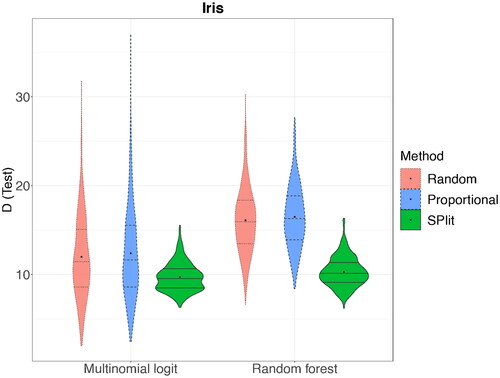
For checking the performance of SPlit on classification problems, consider the famous Iris dataset (Fisher 1936). The Iris dataset has four continuous predictors (sepal length, sepal width, petal length, and petal width) and a categorical response with three levels representing the three types of Iris flowers (setosa, versicolor, and virginica). There are 150 rows in total with 50 rows for each flower type. Following the discussion in Section 3, the flower type is converted into two continuous dummy variables using Helmert coding. Thus, the resulting dataset has six continuous columns. For modeling we will use multinomial logistic regression and random forest. The classification performance will be assessed using the residual deviance (D) defined as(14) $$D:=2\sum _{i=1}^I\sum _{j=1}^J{y}_{ij}·\hspace{0.17em}\text{ln}\hspace{0.17em}\left(\frac{y_{ij}}{{\widehat{p}}_{ij}}\right),$$(14) where I is the number of rows, J the number of classes, $y_{ij}\in \{0,1\}$ is 1 if row i corresponds to class j and 0 otherwise, and ${\widehat{p}}_{ij}$ is the probability that row i belongs to class j as predicted by the model. Note that $0\hspace{0.17em}\text{log}\hspace{0.17em}0$ is taken as 0 by definition.

Figure 8 shows a testing set selected by SPlit. We can see that they are well-balanced among the three classes and the points are well-spread out in the space of the four continuous predictors. We fit multinomial logistic regression and random forest on the training set and then the residual deviance is computed on the testing set. This is then repeated 500 times. Figure 9 shows the deviance results for SPlit, random, and stratified proportional random subsampling. We can see that again SPlit gives significantly better average and worst-case performance compared to both random and stratified proportional random subsampling.

Fig. 8 Visualizing a SPlit subsampling testing set (circles) for the Iris dataset.

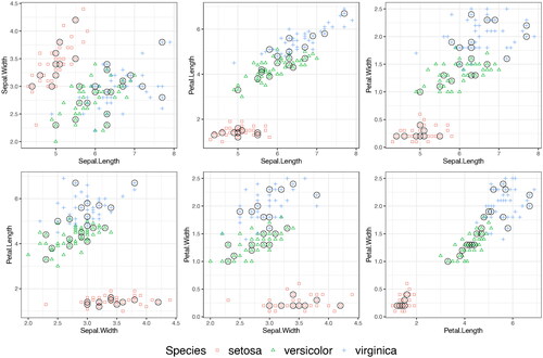
Fig. 9 Distribution of residual deviance (D) over 500 random, stratified proportional random, and SPlit subsampling splits for the Iris dataset.

The foregoing study is repeated for four other datasets: banknote authentication, breast cancer (diagnostic, Wisconsin) (Street, Wolberg, and Mangasarian 1993), cardiotocography (Ayres-de Campos et al. 2000), and glass identification (Evett and Spiehler 1989), all of which can be obtained from the UCI machine learning repository (Dua and Graff 2017). The details of these datasets are summarized in Table 2 and the results on the residual deviance are shown in Figure 10. It is possible to encounter $\infty$ while calculating deviance; for the purpose of plotting, $\infty$ is replaced with the maximum finite deviance obtained from the remainder of the 500 simulations. We can see that SPlit gives a better performance than both random and stratified proportional random subsampling in all the cases. The improvement realized varies over the datasets and modeling methods, but SPlit has a clear advantage over both random and stratified proportional random subsampling.

Fig. 10 Distribution of residual deviance (D) over 500 random, stratified proportional random, and SPlit subsampling splits for the datasets described in Table 2.

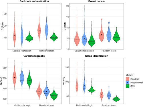
Table 2 Description of datasets considered for classification.

Dataset	Size	Predictors	Response
Banknote authentication	1372 × 5	4 continuous	Categorical (2 levels)
Breast cancer (diagnostic, Wisconsin)	569 × 31	30 continuous	Categorical (2 levels)
Cardiotocography	2126 × 22	20 continuous 1 categorical (3 levels)	Categorical (3 levels)
Glass identification	214 × 10	9 continuous	Categorical (6 levels)

5 Conclusions

Random subsampling is probably the most widely used method for splitting a dataset for testing and training. In this article, we have proposed a new method called SPlit for optimally splitting the dataset. It is done by first finding SP of the dataset and then using an efficient nearest neighbor algorithm to choose the subsamples. They are then used as the testing set and the remaining as the training set. The SP give the best possible representation of the dataset (according to the energy distance criterion) and therefore, SPlit is expected to produce a testing set that is best for evaluating the performance of a model fitted on the training set. The ability of SP to match the distribution of the full data is one of its big advantage over the other deterministic data splitting methods such as CADEX and DUPLEX. We have also extended the method of SP to deal with categorical variables. Thus, SPlit can be applied to both regression and classification problems. We have also briefly discussed on how a sequential application of the SP can be used to generate validation and cross-validation sets, but further development on this topic is left for future research.

We have applied SPlit on several datasets for both regression and classification using different choices of modeling methods and found that SPlit improves the average testing performance in almost all the cases with substantial improvement in the worst-case predictions. The variability in the testing performance metric using SPlit is found to be much smaller than that of random subsampling, which shows that the results and the findings of a statistical study would be much more reproducible if we were to use SPlit.

Acknowledgments

The authors thank to Professor Dan Apley for handling this article as the editor and for his valuable comments and suggestions.

Supplementary materials

code and data.pdf: This file contains R codes to reproduce Figures 2 and 5 as well as links to all the datasets used in Section 4.

Additional information

Funding

This research is supported by a U.S. National Science Foundation grant CBET-1921873.

References

- Ayres-de Campos, D., Bernardes, J., Garrido, A., Marques-de Sa, J., and Pereira-Leite, L. (2000), “Sisporto 2.0: A Program for Automated Analysis of Cardiotocograms,” Journal of Maternal-Fetal Medicine, 9, 311–318.
- Blanco, J. L., and Rai, P. K. (2014), “nanoflann: a C++ header-only fork of FLANN, a library for nearest neighbor (NN) with kd-trees,” available at https://github.com/jlblancoc/nanoflann.
- Bowden, G. J., Maier, H. R., and Dandy, G. C. (2002), “Optimal Division of Data for Neural Network Models in Water Resources Applications,” Water Resources Research, 38, 2–1–2–11. DOI: https://doi.org/10.1029/2001WR000266.
- Breiman, L. (2001), “Random Forests,” Machine Learning, 45, 5–32. DOI: https://doi.org/10.1023/A:1010933404324.
- Brooks, T. F., Pope, D. S., and Marcolini, M. A. (1989), Airfoil Self-noise and Prediction, Washington, DC: NASA.
- Chen, W. Y., Mackey, L., Gorham, J., Briol, F.-X., and Oates, C. (2018), “Stein Points,” in Dy, J. and Krause, A., editors, Proceedings of the 35th International Conference on Machine Learning, Volume 80 of Proceedings of Machine Learning Research, pp. 844–853, Stockholmsmässan, Stockholm Sweden: PMLR.
- Chen, Y., Welling, M., and Smola, A. (2010), “Super-samples From Kernel Herding,” Proceedings of the 26th Conference on Uncertainty in Artificial Intelligence, pp. 109–116.
- Dua, D., and Graff, C. (2017), “UCI Machine Learning Repository,” available at http://archive.ics.uci.edu/ml.
- Elo, I., Rodriguez, G., and Lee, H. (2001), Racial and Neighborhood Disparities in Birthweight in Philadelphia, Washington DC: Annual Meeting of the Population Association of America.
- Evett, I. W., and Spiehler, E. J. (1989), “Rule Induction in Forensic Science,” in Knowledge Based Systems, eds. P. H. Duffin, New York, NY: Halsted Press, pp. 152–160.
- Fang, K. T., and Wang, Y. (1994), Number-Theoretic Methods in Statistics, Boca Raton, FL: Chapman & Hall.
- Faraway, J. J. (2015), Linear Models with R, (2nd ed), Boca Raton, FL: CRC Press.
- Fisher, R. A. (1936), “The Use of Multiple Measurements in Taxonomic Problems,” Annals of Eugenics, 7, 179–188. DOI: https://doi.org/10.1111/j.1469-1809.1936.tb02137.x.
- Flury, B. (1990), “Principal Points,” Biometrika, 77, 33–41. DOI: https://doi.org/10.1093/biomet/77.1.33.
- Friedman, J., Hastie, T., and Tibshirani, R. (2010), “Regularization Paths for Generalized Linear Models Via Coordinate Descent,” Journal of Statistical Software, 33, 1–22. DOI: https://doi.org/10.18637/jss.v033.i01.
- Galvão, R. K. H., Araujo, M. C. U., José, G. E., Pontes, M. J. C., Silva, E. C., and Saldanha, T. C. B. (2005), “A Method for Calibration and Validation Subset Partitioning,” Talanta, 67, 736–740. DOI: https://doi.org/10.1016/j.talanta.2005.03.025.
- Hastie, T., Tibshirani, R., and Friedman, J. (2009), The Elements of Statistical Learning: Data Mining, Inference, and Prediction, New York: Springer.
- Hickernell, F. J. (1999), “Goodness-of-fit Statistics, Discrepancies and Robust Designs,” Statistics and Probability Letters, 44, 73–78. DOI: https://doi.org/10.1016/S0167-7152(98)00293-4.
- Joseph, V. R., Dasgupta, T., Tuo, R., and Wu, C. F. J. (2015), “Sequential Exploration of Complex Surfaces Using Minimum Energy Designs,” Technometrics, 57, 64–74. DOI: https://doi.org/10.1080/00401706.2014.881749.
- Kennard, R. W., and Stone, L. A. (1969), “Computer Aided Design of Experiments,” Technometrics, 11, 137–148. DOI: https://doi.org/10.1080/00401706.1969.10490666.
- Liaw, A., and Wiener, M. (2002), “Classification and Regression by Randomforest,” R News, 2, 18–22.
- Mak, S. (2019), “Support Points. R Package version 0.1.4,” available at https://cran.r-project.org/src/contrib/Archive/support.
- Mak, S., and Joseph, V. R. (2018a), “Projected Support Points: A New Method for High-dimensional Data Reduction,” arXiv preprint: 1708.06897.
- Mak, S., and Joseph, V. R. (2018b), “Support Points,” The Annals of Statistics, 46, 2562–2592.
- May, R., Maier, H., and Dandy, G. (2010), “Data Splitting for Artificial Neural Networks Using SOM-based Stratified Sampling,” Neural Networks, 23, 283 – 294. DOI: https://doi.org/10.1016/j.neunet.2009.11.009.
- Nash, W. J., Sellers, T. L., Talbot, S. R., Cawthorn, A. J., and Ford, W. B. (1994), The Population Biology of Abalone (Haliotis Species) in Tasmania. I. Blacklip Abalone (h. rubra) From the North Coast and Islands of Bass Strait, Technical Report, 48, Tasmania: Sea Fisheries Division, p. 411.
- Niederreiter, H. (1992), Random Number Generation and Quasi-Monte Carlo Methods, Philadelphia, PA: SIAM.
- Owen, A. B. (2013), Monte Carlo Theory, Methods and Examples, available at https://statweb.stanford.edu/∼owen/mc/.
- Reitermanová, Z. (2010), “Data Splitting,” WDS’10 Proceedings of Contributed Papers, Part I, pp. 31–36.
- Snee, R. D. (1977), “Validation of Regression Models: Methods and Examples,” Technometrics, 19, 415–428. DOI: https://doi.org/10.1080/00401706.1977.10489581.
- Stevens, A., and Ramirez-Lopez, L. (2020), An Introduction to the Prospectr Package (R package version 0.2.1).
- Stone, M. (1974), “Cross-validatory Choice and Assessment of Statistical Predictions,” Journal of Royal Statistical Society, Series B, 36, 111–146. DOI: https://doi.org/10.1111/j.2517-6161.1974.tb00994.x.
- Street, W. N., Wolberg, W. H., and Mangasarian, O. L. (1993), “Nuclear Feature Extraction for Breast Tumor Diagnosis,” in Biomedical Image Processing and Biomedical Visualization, Vol. 1905, eds. R. S. Acharya and D. B. Goldgof, pp. 861–870. San Jose, CA: International Society for Optics and Photonics.
- Székely, G. J. and Rizzo, M. L. (2013), “Energy Statistics: A Class of Statistics Based on Distances,” Journal of Statistical Planning and Inference, 143, 1249–1272. DOI: https://doi.org/10.1016/j.jspi.2013.03.018.
- Thodberg, H. H. (1993), “Ace of Bayes: Application of Neural Networks With Pruning,” Technical report, Roskilde, Danmark.
- Tibshirani, R. (1996), “Regression Shrinkage and Selection Via the Lasso,” Journal of the Royal Statistical Society, Series B, 58, 267–288. DOI: https://doi.org/10.1111/j.2517-6161.1996.tb02080.x.
- Wang, H., Yang, M., and Stufken, J. (2019), “Information-based Optimal Subdata Selection for Big Data Linear Regression,” Journal of the American Statistical Association, 114, 393–405. DOI: https://doi.org/10.1080/01621459.2017.1408468.
- Wu, C. F. J., and Hamada, M. S. (2011), Experiments: Planning, Analysis, and Optimization, (2nd ed.) Hoboken, NJ: Wiley.
- Xu, Y., and Goodacre, R. (2018), “On Splitting Training and Validation Set: A Comparative Study of Cross-Validation, Bootstrap and Systematic Sampling for Estimating the Generalization Performance of Supervised Learning,” Journal of Analysis and Testing, 2, 249–262. DOI: https://doi.org/10.1007/s41664-018-0068-2.
- Yeh, I.-C. (1998), “Modeling of Strength of High-performance Concrete Using Artificial Neural Networks,” Cement and Concrete Research, 28,1797–1808. DOI: https://doi.org/10.1016/S0008-8846(98)00165-3.
- Zador, P. (1982), “Asymptotic Quantization Error of Continuous Signals and the Quantization Dimension,” IEEE Transactions on Information Theory, 28, 139–149. DOI: https://doi.org/10.1109/TIT.1982.1056490.