Detecting Changes in Covariance via Random Matrix Theory

Abstract

A novel method is proposed for detecting changes in the covariance structure of moderate dimensional time series. This nonlinear test statistic has a number of useful properties. Most importantly, it is independent of the underlying structure of the covariance matrix. We discuss how results from Random Matrix Theory, can be used to study the behavior of our test statistic in a moderate dimensional setting (i.e., the number of variables is comparable to the length of the data). In particular, we demonstrate that the test statistic converges point wise to a normal distribution under the null hypothesis. We evaluate the performance of the proposed approach on a range of simulated datasets and find that it outperforms a range of alternative recently proposed methods. Finally, we use our approach to study changes in the amount of water on the surface of a plot of soil which feeds into model development for degradation of surface piping.

KEYWORD:

• Changepoint
• Eigenvalue
• Ratio matrices

1 Introduction

There is considerable infrastructure within the oil and gas industry that is on the surface of the ground. These are exposed to changing weather conditions and models are used to estimate the degradation of the assets and direct monitoring. These degradation models rely on estimates of the conditions that the assets are under. As the surrounding soils evolve, so do the absorption properties of the soil. This may result in assets sitting in waterlogged soil when the models are assuming that water drains away. Thus, estimating how these soil properties vary over time, specifically regarding water absorption, is an important task. Soil scientists typically measure water absorption through ground sensors at an individual location. This is not desirable as there may be large areas where assets are located. Recent research has explored video capture to estimate changes in surface water as a surrogate for absorption. Ambient lighting due to time of day and cloud cover hamper traditional mean-based methods for identifying surface water. In this article, we develop a method for identifying changes within an image sequence (viewed as multivariate time series) that are linked to the changing presence of surface water.

One approach to modeling changing behavior in data is to assume that the changes occur at a small number of discrete time points known as changepoints. Between changes, the data can be modeled as a set of stationary segments that satisfy standard modeling assumptions. Changepoint methods are relevant in a wide range of applications including genetics (Hocking et al. 2013), network traffic analysis (Rubin-Delanchy, Lawson, and Heard 2016) and oceanography (Carr et al. 2017). We consider the specific case where the covariance structure of the data changes at each changepoint. While our focus here is on a specific application, the problem has wide applicability. For example, Stoehr, Aston, and Kirch (2020) examine changes in the covariance structure of functional Magnetic Resonance Imaging (fMRI) data, where a failure to satisfy stationarity assumptions can significantly contaminate any analysis, while Wied, Ziggel, and Berens (2013) and Berens, Weiß, and Wied (2015) examine how changes in the covariance of financial data can be used to improve stock portfolio optimization.

The changepoint problem has a long history in the statistical literature, and contains two distinct but related problems, depending on whether the data is observed sequentially (online setting) or as a single batch (offline setting). We focus on the latter and direct readers interested in the former to Tartakovsky, Nikiforov, and Basseville (2014) for a thorough review. In the univariate setting there is a vast literature on different methods for estimating changepoints, and there are a number of state of the art methods (Killick, Fearnhead, and Eckley 2012; Frick et al. 2014; Fryzlewicz 2014; Maidstone et al. 2017).

The literature on detecting changes in multivariate time series has grown substantially in the last few years. In particular, many authors consider changes in the moderate dimensional setting, that is, where the number of the parameters of the model, is of the order of the number of data points. Much of this work considers changes in expectation where the series are uncorrelated (Grundy, Killick, and Mihaylov 2020; Horváth and Hušková 2012). Furthermore a number of authors have examined detecting changes in expectation where only a subset of variables under observation change (Jirak 2015; Wang and Samworth 2018; Enikeeva and Harchaoui 2019). Separately a number of authors have considered changes in second-order structure of moderate dimensional time series models including auto-covariance and cross-covariance (Cho and Fryzlewicz 2015), changes in graphical models (Gibberd and Nelson 2014, 2017) and changes in network structure (Wang, Yu, and Rinaldo 2018).

The problem of detecting changes in the covariance structure has been examined in both the low dimensional and high dimensional setting. In the low dimensional setting ($p\ll n$) Chen and Gupta (2004) and Lavielle and Teyssiere (2006) use a likelihood based test statistic and the Schwarz Information Criterion (SIC) to detect changes in covariance of normally distributed data. Aue et al. (2009) consider a nonparameteric test statistic for changes in the covariance of linear and nonlinear multivariate time series. Matteson and James (2014) study changes in the distribution of (possibly) multivariate time series using a clustering inspired nonparametric test statistic that claims to handle covariances. In the high-dimensional setting, Avanesov and Buzun (2018) and Wang, Yu, and Rinaldo (2017) study test statistics based on the distance between sample covariances, using the operator norm and ${\mathcal{l}}_{\infty }$ norm, respectively. Crucially all of these approaches are focused on exploring the theoretical aspects of the proposed test statistics rather than the practical implications.

In this work we propose a novel method for detecting changes in the covariance structure of moderate dimensional time series motivated by the practical challenges of implementing the approach for estimating changes in soil. In Section 2, we introduce a test statistic inspired by a distance metric intuitively defined on the space of positive definite matrices. The primary advantage of this metric is that under the null hypothesis of no change, it is independent of the underlying covariance structure. This is not the case for other methods in the literature which require users to estimate this. In Section 3, we study the asymptotic properties of this test statistic when, the dimension of the data is of comparable size to (but still smaller than) the sample size. In Section 4, we use these results to propose a new method for detecting multiple changes in the covariance structure of multivariate time series. In Section 5, we study the finite sample performance of the proposed approach on simulated datasets. Finally in Section 6, we use our method to examine how changes in the covariance structure of pixel intensities can be used to detect changes in surface water.

2 Two Sample Tests for the Covariance

Let ${\mathit{X}}_1,\dots ,{\mathit{X}}_n\in {\mathbb{R}}^p$ be independent p dimensional vectors with (2.1) $$\text{cov}\left({\mathit{X}}_i\right)={\Sigma }_{i,p},\text{for}1\le i\le n,$$(2.1) where each ${\Sigma }_{i,p}\in {\mathbb{R}}^{p\times p}$ is full rank. Furthermore, let ${\mathit{X}}_{n,p}$ denote an n × p matrix defined by ${\mathit{X}}_{n,p}:={({\mathit{X}}_1^T,\dots ,{\mathit{X}}_n^T)}^T$. Our primary interest in this article is to develop a testing procedure that can identify a change in the covariance structure of the data over time. For now, let us consider the case of a single changepoint. We compare a null hypothesis of the data sharing the same covariance versus an alternative setting that allows a single change at time τ. Formally we have (2.2) $$H_0:{\Sigma }_0^{*}={\Sigma }_{1,p}=\dots ={\Sigma }_{n,p}$$(2.2) (2.3) $$H_1:{\Sigma }_1^{*}={\Sigma }_{1,p}=\dots ={\Sigma }_{\tau ,p}\ne {\Sigma }_{\tau +1,p}=\dots ={\Sigma }_{n,p}={\Sigma }_2^{*},$$(2.3) where τ is unknown. We are interested in distinguishing between the null and alternative hypothesis, and under the alternative locating the changepoint τ, when the dimension of the data p, is of comparable size to the length of the data, n. In particular we require that for all pairs n, p, the set (2.4) $${\mathcal{T}}_{n,p}(\mathcal{l}):=\{t\in {\mathbb{Z}}^{+}\text{suchthat}\mathcal{l}<t<n-\mathcal{l}\}$$(2.4) is nonempty, where $\mathcal{l}>p$ is a problem dependent positive constant. Note ${\mathcal{T}}_{n,p}(\mathcal{l})$ defines the set of possible candidate changepoints, while $\mathcal{l}$ is the minimum distance between changepoints or minimum segment length. Then for each candidate changepoint $t\in {\mathcal{T}}_{n,p}(\mathcal{l})$, a two sample test statistic T(t) can be used to determine if the data to the left and right of the changepoint have different distributions. If the two sample test statistic for a candidate exceeds some threshold, then we say a change has occurred and an estimator for τ is given by the value $t\in {\mathcal{T}}_{n,p}(\mathcal{l})$ that maximizes T(t).

Let ${\mathit{X}}_{(a+1):b}$ denote the subset of data ${({\mathit{X}}_{a+1}^T,\dots ,{\mathit{X}}_b^T)}^T$ and $\overline{\Sigma }(a,b)$ (or $\overline{\Omega }(a,b)$) be a plug in estimator for the covariance (or precision) of data ${\mathit{X}}_{(a+1):b}$. Then to test for a changepoint at time τ, we can measure the magnitude of the matrix ${\psi }_{\tau ,1}\overline{\Sigma }(0,\tau )-{\psi }_{\tau ,2}\overline{\Sigma }(\tau ,n),$ where ${\left\{{\psi }_{\tau ,1}\right\}}_{\tau =\mathcal{l}+1}^{n-\mathcal{l}}$ and ${\left\{{\psi }_{\tau ,2}\right\}}_{\tau =\mathcal{l}+1}^{n-\mathcal{l}}$ are sequences of normalizing constants. If the spectral norm of this matrix is large, then there is evidence for a change and vice versa. This approach is well represented in the literature, for instance Wang, Yu, and Rinaldo (2017), Aue et al. (2009), Galeano and Peña (2007) measure the difference between sample covariance estimates, while in the high-dimensional setting, Avanesov and Buzun (2018) measures the difference between debiased graphical LASSO estimates. Although this approach is intuitive, it can be challenging to use in practice. A good estimator, $\overline{\Sigma }(a,b)$, will depend on the true covariance of ${\mathit{X}}_{p+1:q}$ which implies that the difference matrix above is dependent on the true covariance of ${\mathit{X}}_{1:n}$. As a result, any test statistic based on a difference matrix must be a function of the underlying covariance, ${\Sigma }_0$, and should be corrected to account for this. For example, Aue et al. (2009), Galeano and Peña (2007) normalize their test statistic using the sample covariance for the whole data, Avanesov and Buzun (2018) use a bootstrap procedure which assumes knowledge of the measure of ${\mathit{X}}_i$ and Wang, Yu, and Rinaldo (2017) use a threshold which is a function of ${\Sigma }_0^{*}$. All these approaches require estimating ${\Sigma }_0$ in practice. This is impractical under the alternative setting, since estimating the segment covariances requires knowledge of the changepoint.

Therefore, it is natural to ask whether there are alternative ways of measuring the distance between covariance metrics. In the univariate setting, a common approach is to evaluate the logarithm of the ratio of the segment variances (Inclan and Tiao 1994; Chen and Gupta 1997; Killick et al. 2010). This is in contrast with the change in expectation problem where it is more common to measure the difference between sample means. In the variance setting a ratio is more appropriate for two reasons. First, since variances are strictly positive, if the underlying variance is quite small then the absolute difference between the values will also be small whereas the ratio is not affected by the scale. Second, under the null hypothesis of no change, the variances will cancel and the test statistic will be independent of the variance. Thus, there is no need to estimate the variance when calculating the threshold.

We propose to extend this ratio idea from the univariate setting to the multivariate setting by studying the multivariate ratio matrix, $\mathit{R}(\mathit{A},\mathit{B}):={\mathit{B}}^{-1}\mathit{A}$, where $\mathit{A},\mathit{B}\in {\mathbb{R}}^{p\times p}$. Ratio matrices are widely used in multivariate analysis to compare covariance matrices (Finn 1974). In particular, we are often interested in functions of the eigenvalues of these matrices (Wilks 1932; Lawley 1938; Potthoff and Roy 1964). Here we are interested in the following test statistic, (2.5) $$T(\mathit{A},\mathit{B})=\sum _{j=1}^p{\left(1-{\lambda }_j(\mathit{R}(\mathit{A},\mathit{B}))\right)}^2+{\left(1-{\lambda }_j^{-1}(\mathit{R}(\mathit{A},\mathit{B}))\right)}^2,$$(2.5) where ${\lambda }_j(\mathit{R}(\mathit{A},\mathit{B}))$ is the jth largest eigenvalue of the matrix $\mathit{R}(\mathit{A},\mathit{B})$. The function T has valuable properties that may not be immediately obvious.

Proposition 2.1.

Let ${\Sigma }_1,{\Sigma }_2\in {\mathbb{R}}^{p\times p}$, be the covariance matrices of data ${\mathit{Z}}_1\in {\mathbb{R}}^{n_1\times p}$ and ${\mathit{Z}}_2\in {\mathbb{R}}^{n_2\times p}$, respectively, and define T as in (2.5). Then we have that, for any covariance matrix ${\Sigma }_0$:

1. T is symmetric that is, $T({\Sigma }_1,{\Sigma }_2)=T({\Sigma }_2,{\Sigma }_1)$;

2. T is symmetric with respect to inversion of matrices that is, $T({\Sigma }_1,{\Sigma }_2)=T({\Sigma }_1^{-1},{\Sigma }_2^{-1})$;

3. If ${\Sigma }_1={\Sigma }_0{\mathit{Z}}_1^T{\mathit{Z}}_1{\Sigma }_0$ and ${\Sigma }_2={\Sigma }_0{\mathit{Z}}_2^T{\mathit{Z}}_2{\Sigma }_0$, then $T({\Sigma }_1,{\Sigma }_2)=T({\mathit{Z}}_1^T{\mathit{Z}}_1,{\mathit{Z}}_2^T{\mathit{Z}}_2)$.

The symmetry property is important for a changepoint analysis as the segmentation should be the same regardless of whether the data is read forwards or backward. The second property states that T is the same whether we examine the covariance matrix or the precision matrix. This ensures that differences between both small and large eigenvalues can be detected. The third property is particularly important as we can translate Proposition 2.1 from two separate datasets ${\mathit{Z}}_1,{\mathit{Z}}_2$ to two subsets of a single dataset ${\mathit{X}}_{n,p}$. This implies that T provides a test statistic which is independent of the underlying covariance of the data. In particular, let $\overline{\Sigma }(a,b)$ be the sample covariance estimate for a subset of data ${\mathit{X}}_{a+1:b}$ that is, $$\overline{\Sigma }(a,b):=\frac{1}{b-a}\sum _{i=a+1}^b{\mathit{X}}_i{\mathit{X}}_i^T.$$

Under the null hypothesis for any $1\le a<b\le n$, ${\mathit{X}}_{a:b}={\Sigma }_0^{1/2}{\mathit{Z}}_{a:b}$ where the covariance of ${\mathit{Z}}_i$ is the identity matrix. Then property 3 implies that for any $1\le \tau \le n$, $T({\mathit{X}}_{1:\tau }^T{\mathit{X}}_{1:\tau },{\mathit{X}}_{\tau +1:n}^T{\mathit{X}}_{\tau +1:n})=T({\mathit{Z}}_{1:\tau }^T{\mathit{Z}}_{1:\tau },{\mathit{Z}}_{\tau +1:n}^T{\mathit{Z}}_{\tau +1:n})$ which is independent of ${\Sigma }_0$. In other words, under the null hypothesis the underlying covariance cancels out (as occurs with the ratio approach in the univariate variance setting). Furthermore, due to the square term, T is a positive definite function. This is necessary to prevent changes canceling out. These properties are clearly not unique to our chosen test statistic T and in fact, there are other possible choices (such as ${\hspace{0.17em}\log \hspace{0.17em}}^{2}x$). However, we argue that for an alternative function $T\prime$ to be appropriate in the changepoint setting, it would also require these properties. Furthermore, this choice of T allows us to analytically derive relevant quantities such as the limiting moments.

It is both possible and interesting to study the properties of this test statistic in the finite dimensional setting (i.e., where p is fixed). However in this work, our focus is on problems where the dimension of the data is of comparable size to the length of the data. Under this asymptotic setting, the eigenvalues of random matrices (and by extension the properties of T) have different limiting behavior and a proper test should take this into account. For example, the two sample Likelihood Ratio Test (as used in Galeano and Peña (2007)) is a function of the log of the determinant of the covariance, or equivalently the sum of the log eigenvalues. In the moderate dimensional setting, this test has been shown to breakdown due to the differing limiting behavior (Bai et al. 2009). Therefore in the next section, we consider the properties of T as a two sample test, and derive the asymptotic distribution under moderate dimensional asymptotics.

3 Random Matrix Theory

We now describe some foundational concepts in Random Matrix Theory (RMT), before discussing how these ideas are used to idenfity the asymptotic distribution of our test statistic under the null hypothesis. RMT concerns the study of matrices where each entry is a random variable. In particular, RMT is often concerned with the behavior of the eigenvalues and eigenvectors of such matrices. Interested readers should see Tao (2012) for an introduction and Anderson, Guionnet, and Zeitouni (2010) for a more thorough review.

A key object of study in the field is the Empirical Spectral Distribution (ESD), defined for a p × p matrix $\mathit{A}$ as (3.6) $$F^{\mathit{A}}(x):=\frac{1}{p}\sum _{j=1}^{p}I({\lambda }_{p-j}(\mathit{A})\le x)$$(3.6) where I is an indicator function. In other words the ESD of $\mathit{A}$ is a discrete uniform distribution placed on the eigenvalues of $\mathit{A}$. Several authors have established results on the limiting behavior of the ESD as the dimension tends to infinity, the so-called Limiting Spectral Distribution (LSD). For example, Wigner (1967) demonstrate that if the upper triangular entries of a Hermitian matrix $\mathit{A}$ have mean zero and unit variance, then $F^{1/\sqrt{p}\mathit{A}}(x)$ converges to the Wigner semicircular distribution.

The LSD of the ratio matrix $\mathit{R}$, was shown to exist in Yin, Bai, and Krishnaiah (1983) and computed analytically in Silverstein (1985). The following two assumptions are sufficient for the LSD of an F matrix to exist.

Assumption 3.1.

Let ${\mathit{X}}_{n_1,p}\in {\mathbb{R}}^{n_1\times p}$ and ${\mathit{X}}_{n_2,p}\in {\mathbb{R}}^{n_2\times p}$ be random matrices with independent not necessarily identically distributed entries $\{{\mathit{X}}_{n_1,i,j},1\le i\le n_1,1\le j\le p\}$ and $\{{\mathit{X}}_{n_2,k,j},1\le k\le n_2,1\le j\le p\}$ with mean 0, variance 1 and fourth moment $1+\kappa$. Furthermore, for any fixed $\eta >0$, (3.7) $$\frac{1}{n_{1}p}\sum _{j=1}^p\sum _{i=1}^{n_1}\mathbb{E}\left|{\mathit{X}}_{n_1,i,j}{|}^4\mathit{I}\right(\left|{\mathit{X}}_{n_1,j,k}\right|\ge \eta \sqrt{n_1})\to 0$$(3.7) (3.8) $$\frac{1}{n_{2}p}\sum _{j=1}^p\sum _{i=1}^{n_2}\mathbb{E}\left|{\mathit{X}}_{n_2,i,j}{|}^4\mathit{I}\right(\left|{\mathit{X}}_{n_2,j,k}\right|\ge \eta \sqrt{n_2})\to 0$$(3.8) as $n_1,n_2,p$ tend to infinity subject to Assumption 3.2.

Assumption 3.2.

The sample sizes n₁, n₂, and the dimension p grow to infinity such that $${\gamma }_{n_1}:=\frac{p}{n_1}\to {\gamma }_1\in (0,1),$$ $${\gamma }_{n_2}:=\frac{p}{n_2}\to {\gamma }_2\in (0,1)\text{and}\mathit{\gamma }:=({\gamma }_1,{\gamma }_2).$$

We refer to the limiting scheme described in Assumption 3.2 as $\mathit{n}\to \infty$.

Let ${\mathit{X}}_{n_1,p},{\mathit{X}}_{n_2,p}$ be matrices satisfying Assumptions 3.1 and 3.2. These assumptions place restrictions on the mean of the data, and the tails of the data. The mean assumption is standard in the literature. If the data has nonzero mean, the data should be standardized, typically by removing the sample mean (assuming the mean is constant). The impact of this on our proposed method is examined in Appendix B.3, supplementary materials. Note that although the matrices ${\mathit{X}}_{n_1,p},{\mathit{X}}_{n_2,p}$ have identity covariance, these results also hold for data with general covariance ${\Sigma }_p$, since by property 3 of Proposition 2.1 the covariance term cancels out under the null hypothesis and we do not require knowledge of ${\Sigma }_p$. Furthermore, let $F_{\mathit{n}}$ denote the ESD of $\mathit{R}({\mathit{X}}_{n_1,p}^T{\mathit{X}}_{n_1,p}/n_1,{\mathit{X}}_{n_2,p}^T{\mathit{X}}_{n_2,p}/n_2)$. Then Silverstein (1985) demonstrate that $F_{\mathit{n}}$ converges almost surely to the nonrandom distribution function (3.9) $$F_{\mathit{\gamma }}(dx)=\frac{1-{\gamma }_2}{2\pi x({\gamma }_1+{\gamma }_{2}x)}\sqrt{(b-x)(x-a)}{I}_{[a,b]}(x)dx\text{as}\mathit{n}\to \infty$$(3.9) (3.10) $$\text{where}h=\sqrt{{\gamma }_1+{\gamma }_2-{\gamma }_1{\gamma }_2},a=\frac{{(1-h)}^2}{{(1-{\gamma }_2)}^2},b=\frac{{(1+h)}^2}{{(1-{\gamma }_2)}^2}.$$(3.10)

The LSD, $F_{\mathit{\gamma }}$ provides an asymptotic centering term for functions of the eigenvalues of random ratio matrices. In particular, for any function f, we have that, $${\mathbb{E}}_{F_n}\left(f\right)=\frac{1}{p}\sum _{i=1}^{p}f\left({\lambda }_i\left(\mathit{R}\left(\frac{1}{n_1}{\mathit{X}}_{n_1,p}^T{\mathit{X}}_{n_1,p},\frac{1}{n_2}{\mathit{X}}_{n_2,p}^T{\mathit{X}}_{n_2,p}\right)\right)\right)$$ $$\hspace{1em}\to \int f(x)d{F}_{\mathit{\gamma }}(x)={\mathbb{E}}_{F_{\mathit{\gamma }}}(f)$$as $\mathit{n}\to \infty$, by the definition of weak convergence. This allows us to account for bias in the statistic as seen in Figure 1.

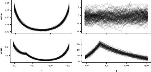
Fig. 1 Test statistic T defined in (2.5) applied to a 100 different datasets before (left) and after standardization (right) using (3.11) under the null setting (top) and alternative setting (bottom) with n = 2000, p = 100, and τ = 666.

The rate of convergence of $\left|{\mathbb{E}}_{F_n}(f)-{\mathbb{E}}_{F_{\mathit{\gamma }}}(f)\right|$ to zero was studied in Zheng (2012) and found to be $1/p$. In particular, the authors establish a central limit theorem for the quantity, $$G_{\mathit{n}}(x):=p\left[F_{\mathit{n}}(x)-F_{\mathit{\gamma }}(x)\right].$$

We can apply this result to our problem in order to demonstrate that our two sample test statistic converges to a normal distribution with known mean and variance terms.

Theorem 3.3.

Let ${\mathit{X}}_{n_1}\in {\mathbb{R}}^{n_1\times p}$ and ${\mathit{X}}_{n_2}\in {\mathbb{R}}^{n_2\times p}$ be random matrices satisfying Assumptions 3.1 and 3.2 and T be defined as in (2.5). Then we have that as $\mathit{n}\to \infty$, $$T\left(\frac{1}{n_1}{\mathit{X}}_{n_1,p}^T{\mathit{X}}_{n_1,p},\frac{1}{n_2}{\mathit{X}}_{n_2,p}^T{\mathit{X}}_{n_2,p}\right)-p\int f^{*}(x)d{F}_{\mathit{\gamma }}(x)$$ $$\to N(\mu (\mathit{\gamma }),{\sigma }^2(\mathit{\gamma }))$$where $f^{*}(x)={(1-x)}^2+{(1-1/x)}^2$, $\mu (\mathit{\gamma })=2K_{3,1}(1-y_2^2/h^2)+2K_{2,1}{y}_2/h+2K_{3,2}(1-y_1^2/h^2)+2K_{2,2}{y}_1/h$, ${\sigma }^2(\mathit{\gamma })=2(K_{2,1}^2+2K_{3,1}^2+K_{2,2}^2+2K_{3,2}^2+J_1{K}_{2,1}/h+$ $(J_1{K}_{2,1})/(h(h^2-1))+(-J_1{K}_{3,1}(h^2+1))/h^2+(-J_1{K}_{3,1})/(h^2(h^2-1))+(J_2{K}_{2,1}2h)/{(h^2-1)}^3+(J_2{K}_{3,1})/h^2+(J_2{K}_{3,1}(1-3h^2))/(h^2{(h^2-1)}^3))$, $K_{2,1}=(2h(1+h^2))/{(1-y_2)}^4-2h/{(1-y_2)}^2$, $K_{2,2}=(2h(1+h^2))/{(1-y_1)}^4-2h/{(1-y_1)}^2$, $K_{3,1}=h^2/{(1-y_2)}^4$, $K_{3,2}=h^2/{(1-y_1)}^4$, $J_1=-2{(1-y_2)}^2,J_2={(1-y_2)}^4$, $h=\sqrt{y_1+y_2-y_1{y}_2}$, $y_1=p/n_1,y_2=p/n_2$.

Using Theorem 3.3, we can properly normalize T such that it can be used within a changepoint analysis. In particular, we have that under the null hypothesis $$T(\overline{\Sigma }(0,t),\overline{\Sigma }(t,n))-p\int f^{*}(x)d{F}_{{\mathit{\gamma }}_{t/n}}\to N(\mu ({\mathit{\gamma }}_{t/n}),{\sigma }^2({\mathit{\gamma }}_{t/n}))$$weakly as n, p tend to infinity, where ${\gamma }_{t/n}:=(p/t,p/(n-t))$ and $f^{*}$ is as defined in Theorem 3.3. Thus, we use the normalized test statistic, $\tilde{T}$, (3.11) $$\begin{array}{c}\tilde{T}(t):={\sigma }^{-1/2}({\mathit{\gamma }}_{t/n})(T(\overline{\Sigma }(0,t),\overline{\Sigma }(t,n))\\ \hspace{1em}-p\int f^{*}(x)d{F}_{{\mathit{\gamma }}_{t/n}}-\mu ({\mathit{\gamma }}_{\tau /n})),\end{array}$$(3.11) which under the null hypothesis converges pointwise to a standard normal random variable.

The asymptotic moments of the test statistic, T, depend on the parameter ${\mathit{\gamma }}_{t/n}$ and, as t approaches p (or equivalently n – p) the mean and variance of the test statistic dramatically increase. In the context of changepoint analysis, this implies that the mean and variance increase at the edges of the data. We note that this is a common feature of changepoint test statistics. We can significantly reduce the impact of this by the above standardization. This can be seen empirically in Figure 1. After standardization, the test statistics for the series with no change, do not appear to have any structure. Similarly, the test statistics for the series with a change show a clear peak at the changepoint. Importantly we can now easily distinguish the test statistic under the null and alternative hypotheses, and this normalization does not require knowledge of the underlying covariance structure.

4 Practical Considerations

Before we can apply our method to real and simulated data, we need to address three practical concerns, namely we must select a threshold for rejecting the null hypothesis, determine an appropriate minimum segment length and address the issue of multiple changepoints.

4.1 Threshold for Detecting a Change

First, we need to select an appropriate threshold for rejecting the null hypothesis. We choose to use the asymptotic distribution of the test statistic on a pointwise basis, that is for each $\mathcal{l}<t<n-\mathcal{l}$ we say that $\tilde{T}(t)\approx Z_t$, where Z_t is a standard normal variable. This do not take into account whether or not we are in the limiting regime and as a result, the method may be unreliable if p is small (indeed we observe this pattern in Section 5). We then use a Bonferroni correction (Haynes 2013) to control the probability that any Z_t exceeds a threshold α. In particular, for a given significance level α, we reject the null hypothesis for a single change in data of length n if $\tilde{T}(t)>q(1-\alpha /n)$ for some $\mathcal{l}<t<n-\mathcal{l}$, where $q(\alpha )$ is the αth quantile of the standard normal distribution. In the case of multiple changepoints, we use $q(1-2\alpha /n(n+1))$ to account for the extra hypothesis tests. We note that a Bonferroni correction is known to be conservative and as a result, using this approach may have poor size (again results from the simulation study validate this concern). Ideally, one would take account of the strong dependence between consecutive test statistics to get a better threshold, but this is challenging given the nonlinear nature of the test statistic. Further work may wish to investigate whether finite sample results which exploit this dependence can be derived. Alternatively practitioners could use several different thresholds and ascertain the appropriate threshold for a particular application at hand as demonstrated in Lavielle (2005).

4.2 Minimum Segment Length

The test statistic proposed relies on an appropriate choice for the minimum segment length parameter, $\mathcal{l}$. Too small and the covariance estimates in the small segments will elicit false detection, too large and the changepoints will not be localized enough to be useful.

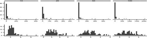
In many applications, domain specific knowledge may be used to increase this parameter. However, it is also important to consider smallest value that will give reliable results in the general case. The minimum segment length must grow sufficiently fast to ensure that $\tilde{T}(t)$ converges to a normal distribution. Outside the asymptotic regime, it is possible for the ratio matrix to have very large eigenvalues. Thus, for candidate changepoints t close to p (or by symmetry n – p), the probability of observing spuriously large values of $\tilde{T}(t)$ becomes much larger. This can be seen in Figure 2. When $\mathcal{l}=p$ (the smallest possible value), we observe extremely large values of the test statistic, that would make identifying a true change almost impossible. However, when $\mathcal{l}=4p$, the test statistic behaves reliably. Thus, we need $p/(p+{\mathcal{l}}_{n,p})$ to converge to ${\gamma }_{\mathcal{l}}\in (0,1)$ or equivalently ${\mathcal{l}}_{n,p}=\mathcal{O}(p)$ for the asymptotic results to hold. In Appendix B.1, supplementary materials, we analyze the effect of different sequences in the finite sample setting via a simulation study. Based on these results, we recommend using a default value of $\max \{4p,30\}$, however note that as p grows to a moderate size, smaller values can be taken without any corresponding decrease in performance.

Fig. 2 Histogram of values of $\underset{\mathcal{l}<t<n-\mathcal{l}}{\max }\tilde{T}(t)$ applied to 100 datasets of length n = 2000 with no change for $p=\{10,20,50,100\}$ with $\mathcal{l}=p$ (top) and $\mathcal{l}=4p$ (bottom).

4.3 Multiple Changepoints

Finally, we also consider the extension to multiple changes. In this setting, extend the single changepoint setting considered previously to a set of m unknown ordered changepoints, $\mathit{\tau }:=\{0={\tau }_0,{\tau }_1,\dots {\tau }_m,{\tau }_{m+1}=n\}$ such that, ${\Sigma }_i={\Sigma }_k^{*},{\tau }_k<i\le {\tau }_{k+1},1\le k\le m+1,$ and ${\Sigma }_i$ is the covariance matrix of the ith time-vector. We are interested in estimating the number of changes m, and the set of changepoints $\mathit{\tau }$. The classic approach to this problem, is to extend a method defined for the single changepoint setting to the multiple changepoint setting, via an appropriate search method such as dynamic programming or binary segmentation. For this work, we cannot apply the dynamic programming approach (Killick, Fearnhead, and Eckley 2012), which minimizes the within segment variability through a cost function for each segment. This is because our distance metric is formulated as a two-sample test and cannot be readily expressed as cost function for a single segment. Therefore, we use the classic binary segmentation procedure (Scott and Knott 1974). The binary segmentation method extends a single changepoint test as follows. First, the test is run on the whole data. If no change is found then the algorithm terminates. If a changepoint is found, it is added to the list of estimated changepoints and, the binary segmentation procedure is then run on the data to the left and right of the candidate change. This process continues until no more changes are found. Note the threshold, v, and the minimum segment length, $\mathcal{l}$, remain the same. We note that a number of extensions of the traditional binary segmentation procedure have been proposed in recent years (Olshen et al. 2004; Fryzlewicz 2014). Although we do not use these search methods in our simulations, due to additional optional parameters that affect performance, it is not difficult to incorporate our proposed test statistic into these adaptations of the original binary segmentation approach. The full proposed procedure is described in Algorithm 1.

Algorithm 1:

Ratio Binary Segmentation(RatioBinSeg)

Input: Data matrix $\mathit{X}$, (s, e), $\mathcal{C}$, minseglen $\mathcal{l}$, significance level α $$v=1-\frac{\alpha }{n^2};$$for $s+\mathcal{l}\le \tau \le e-\mathcal{l}$ do

$\mathit{\gamma }:=(\frac{p}{\tau },\frac{p}{n-\tau })$; $\tilde{T}(\tau ):={\sigma }^{-1/2}(\mathit{\gamma })(T(\overline{\Sigma }(s,\tau ),\overline{\Sigma }(\tau ,e))-p\int f^{*}(x)d{F}_{\mathit{\gamma }}-\mu (\mathit{\gamma }))$;end $$\widehat{\tau }:=\underset{s+\mathcal{l}<\tau <e-\mathcal{l}}{\arg \max }\tilde{T}(\tau );$$ if $\tilde{T}(\widehat{\tau })>v$ then

${\mathcal{C}}_l:=$ RatioBinSeg $(\mathit{X},(s,\tau ),\mathcal{C},\mathcal{l},\alpha )$;

${\mathcal{C}}_r:=$ RatioBinSeg $(\mathit{X},(\tau ,e),\mathcal{C},\mathcal{l},\alpha )$; $$\mathcal{C}=\mathcal{C}\cup \left\{\widehat{\tau }\right\}\cup {\mathcal{C}}_l\cup {\mathcal{C}}_r;$$end

Output: Set of changepoints $\mathcal{C}$.

5 Simulations

In this section, we compare our method with existing methods in the literature, namely the methods of Wang, Yu, and Rinaldo (2017), Aue et al. (2009), and Galeano and Peña (2007), which we refer to as the Aue, Galeano and Wang methods, respectively. We do not consider Avanesov and Buzun (2018) as this method is intended for the high-dimensional setting and so would be an unfair comparison. Software implementing these methods is not currently available and as a result, we have implemented each of these methods according to the descriptions in their respective papers. All methods, simulations, visuals and analysis have been implemented in the R programming language (R Core Team 2020). The code to repeat our experiments is available at https://github.com/s-ryan1/Covariance_RMT_simulations.

Simulation studies in the current literature for changes in covariance structure are very limited. Wang, Yu, and Rinaldo (2017) do not include any simulations. Aue et al. (2009) and Avanesov and Buzun (2018) only consider the single changepoint setting, and do not consider random parameters for the changes. Furthermore to our knowledge, no papers compare the performance of different methods. While theoretical results are clearly important, it is also necessary to consider the finite sample performance of any estimator, and we now study the finite sample properties of our approach on simulated datasets. Further details on the general setup of our simulations are given in Appendix A, supplementary materials. Note that the significance thresholds for each method are set to be favorable to competing methods and we anticipate that performance would decrease in practical settings.

We begin by analyzing the performance of our approach (which we refer to as the Ratio method) in the single changepoint setting. This allows us to directly examine the finite sample properties of the method, such as the power and size, as well as investigate how violations to our assumptions, such as autocorrelation and heavy tailed errors impact the method. We then compare our approach with current state of the art methods for detecting multiple changepoints. Results for assessing the chosen default values for the minimum segment length parameter in Section 4, as well as a comparison of different methods in the single changepoint setting, are given in Appendix B, supplementary materials. These demonstrate that, overall, the Ratio, Galeano and Aue methods are well peaked whereas the Wang method is not leading to accurate changepoint localization. In both settings, the localization of the changepoints is more accurate for our approach than the Aue et al. (2009) method while also being applicable to larger values of p. However, the Galeano method does produce more defined peaks than the Ratio method. This results in better localization but unfortunately does not produce better overall results due to the peaks not exceeding the asymptotic threshold. This could be rectified by using a smaller (nonasymptotic) threshold. Finally, comparisons for the Ratio method based on whether or not the mean is known (under the null and alternate hypotheses) are provided in Appendix B, supplementary materials. These results show that centering the data by subtracting the sample mean has a small impact on the performance of the method.

Performance Metrics

In the single changepoint setting, we are interested in whether the Ratio approach provides a valid hypothesis test. Therefore, for a given set of simulations, we measure how often the method incorrectly rejects the null (Type 1 error) and how often the method fails to correctly reject the null (Type 2 error). Furthermore, under the alternative hypothesis, we measure the absolute difference between the estimated changepoint and the true change, and refer to this throughout as the Changepoint Error. For the multiple changepoint setting, we use $\mathit{\tau }:=\{{\tau }_1,\dots ,{\tau }_m\}$ and $\widehat{\mathit{\tau }}:=\{{\widehat{\tau }}_1,\dots ,{\widehat{\tau }}_{\widehat{m}}\}$ to denote the set of true changepoints and the set of estimated changepoints, respectively. We say that the changepoint τ_i has been detected correctly if $|{\widehat{\tau }}_j-{\tau }_i|\le h$ for some $1\le j\le \widehat{m}$ and denote the set of correctly estimated changes by ${\mathit{\tau }}_c$. Then we define the True Positive Rate (TPR) and False Positive Rate (FPR) as follows, $$\text{TPR}:=\frac{\left|{\mathit{\tau }}_c\right|}{\left|\mathit{\tau }\right|},\text{FPR}:=\frac{\left|\widehat{\mathit{\tau }}\right|-\left|{\mathit{\tau }}_c\right|}{\left|\widehat{\mathit{\tau }}\right|}.$$

A perfect method will have a TPR of 1 and FPR of 0. We set h = 20 although it should be noted that in reality the desired accuracy would be application specific and dependent on the minimum segment length l. Although, while the specific values vary with h the conclusions of the study do not. We also consider whether or not the resulting segmentation allows us to estimate the true underlying covariance matrices, and define the Mean Absolute Error (MAE) as $$\mathit{MAE}:=\frac{1}{n}\sum _{i=1}^n{\Vert {\widehat{\Sigma }}_i-{\Sigma }_i\Vert }_1.$$

5.1 Finite Sample Properties

We begin by examining the performance of our proposed approach on normally distributed datasets with length $n=\{500,1000,2000,5000\}$ and dimension $p=\{10,50,100\}$. Based on results from Section 4.2, the minimum segment length was set to 4p. For each n, p pair, we generated 1000 datasets with a single change at time $n/2$ as follows (5.12) $${\mathit{X}}_i\sim \mathcal{N}(0,{\mathit{I}}_p)\text{for}1\le i\le n/2\text{and}{\mathit{X}}_i\sim \delta \mathcal{N}(0,{\mathit{I}}_p)\text{for}i>n/2,$$(5.12) where ${\mathit{I}}_p$ is the identity matrix of dimension p and $\delta =\{1,1.05,1.1,1.15,1.2\}$. Note since our approach is invariant to the covariance of the data under the null hypothesis, this is equivalent to generating the data with some unknown covariance. We use the approach described in Section 4.1 to select the threshold with $\alpha =0.05$. 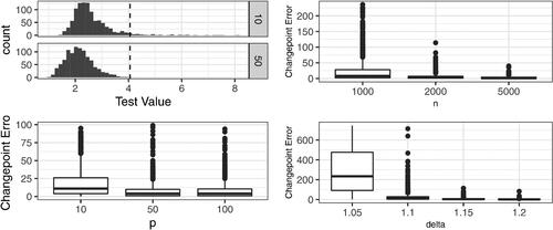A histogram of the test statistic values under the null hypothesis $(\delta =1)$ for n = 2000 and p = 10, 50 is shown in Figure 3. For p = 10, we observe a right-skewed distribution, however, this effect is not present for p = 50, indicating that we may not entered the limiting regime when p = 10. However, when we compute the FPR for each n, p pair (Table E.4, supplementary materials) we note that across all dimensions, we observe low numbers of false positives. In particular, for p = 50 and p = 100 the method is conservative. This highlights an important difference between theoretical convergence and practical performance. Although at p = 10 the theoretical limiting distribution has not been reached, the practical results show that the false positive rate is not inflated. We measure the power and accuracy of our method via the True Positive Rate (TPR) and the absolute difference between the estimated change and the true change (Changepoint Error). The TPR is given in Table E.4, supplementary materials for $\delta =1.1$. As n, p increases the probability of detection increases. However, for smaller values of n/p, the method can have less power, such as $n=1000,p=100$ and $n=500,p=50$. In these cases, using less data gives a better detection rate, implying that the method inefficiently uses the data and a high dimensional approach may be preferable. Changepoint errors are given in Figure 3. As $n,p,\delta$ increase, the method more accurately locates the changepoint, as we would expect.

Fig. 3 Clockwise from Top Left: Test values for p = 10, 50, dashed line indicates threshold. For higher dimensions we observe less outliers. Changepoint error under increasing data length (n, $\delta =1.15$, p = 50), dimension (p, $\delta =1.1$, n = 5000), and size of change (δ, p = 50, n = 2000). The method becomes more accurate as these increase.

Serial Dependence

Our method does not allow for dependence between successive data points. To measure the impact of serial dependence, we generated data, (5.13) $$\begin{array}{c}{\mathit{X}}_i\sim \varphi {\mathit{X}}_{i-1}+{ϵ}_i\text{for}1\le i\le n/2\mathrm{ }\text{and}\\ {\mathit{X}}_i\sim \varphi {\mathit{X}}_{i-1}+\delta {ϵ}_i\text{for}i>n/2\end{array}$$(5.13) where ${ϵ}_i\sim \mathcal{N}(0,{\mathit{I}}_p)$, n = 2000, p = 50 and $\delta =\{1,1.1,1.2\}$ and $\varphi =\{0,.1,.3,.6,.9\}$. Results from this analysis are shown in Figure 4. Focusing on the top left plot, we can see that even under the null the test values increase as the autocorrelation increases, and we find that for $\varphi \ge 0.3$ the proposed threshold is invalid, with FPRs of approximately 1. Thus, the test is invalid and will produce spurious false positives. This is well known in the univariate changepoint literature (Shi et al. 2021) and can be mitigated by scaling the threshold by the autocorrelation observed.

Fig. 4 Clockwise from Top Left: Test statistic values for AR(1) data with $\delta =1,1.1$, dashed line indicates threshold. Changepoint Error for AR(1) data ($\delta =1.1)$. Changepoint Error for different error distributions. Test values for different error distributions, dashed line indicates threshold. As autocorrelation and probability of outliers increases the method becomes less accurate.

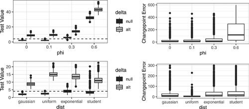
Similarly the power and accuracy of our method decreases when changepoints are present. Figure 4 shows the separation between test statistic value under the null and alternative hypothesis. If these values are well separated then the method will have good power given a valid threshold. We find that the separation between the null and alternative distributions decreases and thus changepoint error increases as $\varphi$ increases. These results show that as autocorrelation increases, our method becomes less accurate as expected.

Model Misspecification

Our method places assumptions on the data which may not hold in practice. To measure the impact of this we generated data (5.14) $${\mathit{Y}}_i=\{\begin{array}{c}{\mathit{X}}_i-{\mu }_{f^k}\text{where}{x}_{ij}\sim F_k\text{for}1\le i\le n/2,1\le j\le p\hfill \\ \delta ({\mathit{X}}_i-{\mu }_{f^k})\text{where}{x}_{ij}\sim F_k\text{for}i>n/2,1\le j\le p\hfill \end{array}$$(5.14)

$F_1=\mathcal{N}(0,1),F_2=$ Uniform $(-1/2,1/2),F_3=$ Exponential(1), $F_4=$ Student t(5), n = 2000, p = 50 and $\delta =1,1.1,1.2$. Note the exponential and t-distributions do not satisfy Assumption 3.1 and as a result, the threshold is invalid producing FPRs of 0.512 and 0.248, respectively. Interestingly, although the t-distribution has heavier tailed errors than the exponential distribution, it gives a lower FPR. This is likely due to the skewness of the exponential distribution. We find that the method has less power for the heavier tailed distributions (Figure 4), as again, the distributions under the null and alternative overlap more. This pattern is repeated for the changepoint error. Thus, the method will be less accurate in the presence of heavy tailed errors. Note that the test statistic can still be used for heavy tailed data, the threshold for identification of a change simply needs to be modified to account for this. This could be achieved by theoretically identifying the new limiting distribution or by using data-driven threshold methods as in Lavielle (2005).

5.2 Multiple Change Points

We now compare the Ratio approach with other methods on simulated datasets with multiple changepoints. We consider datasets with 4 changepoints, uniformly sampled with minimum segment length $p\hspace{0.17em}\log \hspace{0.17em}n$, where $p=\{3,10,30,100\}$ and $n=\{200,500,1000,2000,5000\}$. Covariance matrices are generated so that the distance between consecutive covariance matrices is sufficiently large to detect a change. We consider two separate metrics, $$d_1(\mathit{A},\mathit{B})=\sum _{j=1}^p{\lambda }_j^2(\mathit{A}-\mathit{B})\text{and}{d}_2(\mathit{A},\mathit{B})=\sum _{j=1}^p{({\lambda }_j^2({\mathit{A}}^{-1}\mathit{B})-1)}^2,$$where d₁ matches the assumptions from Wang, Yu, and Rinaldo (2017), while d₂ matches the distance metric used by T. As such, the first set of simulations should favor the Wang method. Full details for how the covariances were generated are provided in Appendix A.2, supplementary materials. For each (n, p) pair and distance metric, we generated 1000 datasets and applied our method, the Aue et al. (2009) method, the Wang, Yu, and Rinaldo (2017) method and Galeano and Peña (2007) method to each dataset. Due to its computational complexity, we do not run the Aue method for $p>10$. Using the resulting segmentations, we then calculated the error metrics for each method and report these in Tables 1 and 2. The worst performers across all metrics are the Galeano and Wang methods. Notably the true positive rate for the Wang method decreases as p grows. This is in striking contrast with the other methods which become more accurate for larger values of p as one may expect. This may be due to the fact that the Wang method only considers the first principal component of the difference matrix, ignoring the remainder of the spectrum or the bias issue identified in Appendix B.2, supplementary materials. The high false positive rate indicates that adapting the threshold would not lead to improved results. The Galeano performance is expected due to the threshold issue highlighted in the single changepoint section (Appendix B.2, supplementary materials) being exacerbated by the smaller sample sizes between changepoints. What is not expected is the larger increase in FPR relative to TPR. This indicates that the test statistic may struggle to maintain its clear peaks when multiple changepoints are present. The Ratio and Aue methods are more closely matched. We can see that the Ratio method is the more conservative of the two, producing a lower FPR and corresponding lower TPR when p and n are smaller. This is unsurprising since our results in the single changepoint case found that the Ratio method can be less reliable when p < 10. For scenarios with p > 30, the Ratio approach is extremely accurate. This indicates that for problems with smaller dimensions, the Aue method may be preferable, while the approach presented here is suitable for larger dimensions.

Table 1 Results (to 2dp) from multiple changepoint simulations based on Ratio constraints described in Appendix A.2, supplementary materials.

		FPR				MAE				TPR
p	n	Aue	Ratio	Wang	Galeano	Aue	Ratio	Wang	Galeano	Aue	Ratio	Wang	Galeano
3	500	0.36	0.24	0.63	0.00	26.05	26.52	42.82	55.67	0.55	0.38	0.51	0.00
	1000	0.48	0.28	0.77	0.02	18.44	15.36	36.81	48.97	0.59	0.48	0.48	0.01
	2000	0.54	0.31	0.85	0.09	12.78	7.65	32.14	43.95	0.63	0.60	0.44	0.03
	5000	0.59	0.31	0.90	0.23	7.95	2.93	23.85	36.66	0.65	0.68	0.45	0.06
10	500	0.25	0.16	0.27	0.00	304.00	303.63	316.80	780.50	0.56	0.55	0.51	0.01
	1000	0.32	0.13	0.43	0.04	167.59	127.71	243.70	678.34	0.69	0.75	0.54	0.01
	2000	0.34	0.10	0.53	0.09	99.52	46.44	186.26	594.56	0.76	0.87	0.58	0.04
	5000	0.37	0.09	0.62	0.21	58.09	16.62	123.34	492.97	0.80	0.91	0.61	0.07
30	2000		0.02	0.32	0.09		143.43	1078.25	3079.91		0.98	0.45	0.05
	5000		0.02	0.31	0.22		51.37	525.14	2357.40		0.99	0.56	0.10
100	5000		0.00	0.45	0.26		199.51	7769.79	16281.43		1.00	0.31	0.13

NOTE: For smaller values of p, the Ratio provides lower FPR and lower TPR than the Aue method. However, for larger values of p the Ratio method is the top performer, indicating a tradeoff between the methods. Confidence intervals for mean values are provided in Table E.2, supplementary materials. The bold values highlight the best performer in each comparison.

Table 2 Results from multiple changepoint simulations based on assumptions in Wang, Yu, and Rinaldo (2018) described in Appendix A.2, supplementary materials.

		FPR				MAE				TPR
p	n	Aue	Ratio	Wang	Galeano	Aue	Ratio	Wang	Galeano	Aue	Ratio	Wang	Galeano
3	500	0.30	0.10	0.64	0.04	21.21	16.99	41.76	37.55	0.75	0.64	0.41	0.05
3	1000	0.40	0.14	0.80	0.15	16.40	9.89	37.33	28.43	0.77	0.71	0.35	0.10
3	2000	0.47	0.16	0.88	0.21	12.15	5.49	30.60	22.03	0.77	0.76	0.30	0.16
3	5000	0.52	0.17	0.92	0.27	7.55	2.27	22.21	15.40	0.77	0.80	0.28	0.25
10	500	0.35	0.23	0.39	0.00	226.71	244.77	265.47	328.85	0.35	0.28	0.19	0.00
10	1000	0.45	0.24	0.62	0.01	141.09	141.19	201.80	251.90	0.46	0.40	0.14	0.00
10	2000	0.48	0.24	0.75	0.04	91.04	71.25	147.13	200.19	0.54	0.53	0.13	0.01
10	5000	0.48	0.19	0.80	0.14	50.98	22.63	90.40	153.18	0.63	0.70	0.14	0.04
30	2000		0.03	0.58	0.08		135.30	1117.87	1271.95		0.96	0.05	0.03
30	5000		0.03	0.78	0.19		42.62	666.52	840.05		0.98	0.06	0.07
100	5000		0.00	0.18	0.26		163.02	7767.18	6082.83		1.00	0.01	0.22

NOTE: For smaller values of p, the Ratio provides lower FPR and lower TPR than the Aue method. However, for larger values of p the Ratio method is the top performer, indicating a tradeoff between the methods. Confidence intervals for mean values are provided in Table E.3, supplementary materials. The bold values highlight the best performer in each comparison.

6 Detecting Changes in Moisture Levels in Soil

In this section, we investigate whether changes in the covariance structure of soil data correspond with shifts in the amount of moisture on the soil. There is significant interest in developing new techniques to better understand when water is present, how water is absorbed and the general modeling of surface water (Cândido et al. 2020; Burak et al. 2021). This is an important question and is relevant to a variety of industrial applications such as farming, construction and the oil and gas industry (Hillel 2003). A widely used approach is to place probes at different depths and locations in the soil which measure the level of moisture. To measure across a site more easily, scientists are investigating the use of cameras to capture the soil surface as a surrogate for moisture.

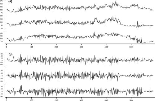
We analyze images from a preliminary experiment studying moisture on the surface of the soil provided privately to the authors by Anette Eltner from TU Dresden following discussions around modeling challenges for soil erosion with the Lancaster Environment Centre. A camera was placed over a large plot of soil and took a set of 589 pictures over the experiment. The images are taken at 10 sec intervals of a total of just over 98 min. At different times, different amounts of rainfall are artificially added to the field site and the amount of water on the soil surface changes (Eltner et al. 2017). We wish to segment the data into periods of dry, wet and surface water. The intensity of a set of pixels over time is shown in Figure 5. We can see that the mean level is clearly nonstationary. This nonstationary behavior may be attributed to two causes, changes in the background light intensity (due to a cloud passing by) and changes in the wetness of the soil which changes how much light is reflected. Since changes in the mean intensity are not necessarily associated with changes in the wetness, we instead focus on changes in the covariance structure. If pixels become wet we would expect that the correlation between the pixels should increase as they become more alike as the surface becomes uniformly water instead of the variable soil surface. Thus, changes in the covariance structure of the pixels may correspond with changes in the wetness.

Fig. 5 (a) Raw grayscale intensities for three pixels. (b) Standardized intensities for the same three pixels.

The data consists of 589 images and we analyze two subsets with p = 10, 30 pixels within a target area of the image. The original images are in color but were transferred to grayscale for computational purposes. We run a multiple changepoint analysis on the smaller subset using our approach as well as the Aue and Wang methods. We also ran a multiple changepoint analysis on the larger subset.

In order to analyze the covariance structure of the data, we first need to transform the data to have stationary mean. Estimating the mean of this series is challenging as there is stochastic volatility and the smoothness of the function appears to change over time. As a result, standard smoothing methods such as LOESS and windowed mean estimators may be inappropriate. We use a Bayesian Trend Filter with Dynamic Shrinkage (Kowal, Matteson, and Ruppert 2019), implemented in the DSP R package (Kowal 2020), which is robust to these issues. We then take the residuals. The transformed data for a subset of the pixels can be seen in Figure 5. The minimum segment length is set to 25. Considering the results in Figure B.1, choosing a minimum segment length of 25 will increase the false positive rate under no changepoints. We need to balance this against the need to detect potentially short-lived periods of change. The thresholds for significance for each method were again set to the defaults as discussed in the previous section. The results of this analysis are shown in Table 3.

Table 3 Detected changepoints for each of the three methods when applied to the soil image data.

Method	Small subset (p = 10)	Larger subset (p = 30)
Aue	66, 101, 243, 354, 451, 514, 589	NA
Wang	52,79, 184, 237, 445	445
Ratio	49, 77, 244, 347, 452, 493, 532,562	64, 125, 184, 255, 340, 450, 527

NOTE: The dimension of the larger subset means the Aue method can detect at most one changepoint.

To validate our results we worked with scientists studying this data and identified three clear time points where there is a substantial change in the amount of water on the surface at the relevant pixels. The first change is somewhat gradual going from very dry at time t = 64 to very wet from time t = 76. The second and third changes are more abrupt, with a substantial increase in the amount of water at time t = 350 and a corresponding sharp decrease at time t = 450. The Aue method reports 7 changepoints, the Wang method reports 5 changepoints and our method locates 8 changepoints. All methods detect the first and last changes. However, the Wang method does not detect any change near the second anticipated changepoint. All of the methods appear to overfit changepoints, in the sense that they report changes that do not correspond with clear changes in the amount of water on the surface. For our method and the Aue method, the majority of these overfitted changes occur when the soil is dry (before t = 64 and after t = 450). During these periods the scientists were moving around the site increasing the variability in the amount of light exposure from image to image which may explain these nuisance changes. However, we also acknowledge that, for the Ratio method, this could be due to the modified segment length increasing the false alarm rate.

For the larger dimension dataset, the minimum segment length was set to 60 (2p) and the thresholds were set to their defaults. As p is of a moderate size, the 4p minimum segment length is quite conservative (Figure B.1) so we can reduce the minimum segment length without increasing the false positive rate. For p = 30, a minimum segment length of 2p gives a null false positive rate around 0.05. The results were broadly similar for our method and quite different for the Wang method. Our approach reports 6 changes again detecting the three obvious changes in the video. We note that the reduced number of changepoints is primarily due to the increased minimum segment length. The Wang method only reports a single changepoint. This drop in reported changes is caused by the largest eigenvalue of the sample covariance being much larger. As a result, the threshold for detecting a change is 3.5 times larger to account for this and consequently, it appears that the method loses power.

On a practical note, when reducing the minimum segment length one needs to be careful on interpretation of changepoints that are closer than 4p. If the changes in covariance structure are small then these could be false alarms due to the variance of the covariance estimate for small samples rather than true changepoints. Practitioners can use Figure B.1 to guide decisions around minimum segment lengths and the risk of false alarms.

7 Conclusion

In this work, we have presented a novel test statistic for detecting changes in the covariance structure of moderate dimensional data. This geometrically inspired test statistic has a number of desirable properties that are not features of competitor methods. Most notably our approach does not require knowledge of the underlying covariance structure. We use results from Random Matrix Theory to derive a limiting distribution for our test statistic. The proposed method outperforms other methods on simulated datasets, in terms of both accuracy in detecting changes and estimation of the underlying covariance model. We then use our method to analyze changes in the amount of surface water on a plot of soil. We find that our approach is able to detect changes in this dataset that are visible to the eye and locates a number of other changes. It is not clear whether these changes correspond to true changes in the surface water and we are investigating this further.

While our method has a number of advantages, it is important to recognize some limitations. First, our method requires calculating the inverse of a matrix at each time point, which is a computationally and memory intensive operation. As a result, our approach is challenging for larger datasets that can be considered by other methods, which only require the first principle component. This could be mitigated by novel solutions to solving inverse matrices alongside GPU computation. However, as we demonstrate through simulations, there are a wide range of settings where our method produces considerable better results for a marginal increase in computational time. Finally we note that a limitation of our method is that the minimum segment length is bounded below by the dimension of the data. This means that the method cannot be applied to tall datasets (p > n) or datasets with short segments. It may be that our method could be adapted to these settings by applying recent advances in high dimensional covariance estimation, and replacing the empirical estimate of the covariance matrix with these.

Supplementary Materials

The supplemental materials contain (1) further details on the simulation study, (2) additional simulations, (3) auxillery results, (4) proof of main results, (5) standard errors for the results in section 5, (6) further details on the application.

Acknowledgments

The authors would like to thank Anette Eltner for providing the substantive application considered here as well as John Quinton and Mike James for the discussion and interpretation of the results.

Additional information

Funding

The authors gratefully acknowledge funding from EP/L015692/1, EP/R01860X/1, and NE/T012307/1.

References

- Anderson, G. W., Guionnet, A., and Zeitouni, O. (2010), An Introduction to Random Matrices (Vol. 118), Cambridge: Cambridge University Press.
- Aue, A., Hörmann, S., Horváth, L., and Reimherr, M. (2009), “Break Detection in the Covariance Structure of Multivariate Time Series Models,” The Annals of Statistics, 37, 4046–4087. DOI: 10.1214/09-AOS707.
- Avanesov, V., and Buzun, N. (2018), “Change-Point Detection in High-Dimensional Covariance Structure,” Electronic Journal of Statistics, 12, 3254–3294. DOI: 10.1214/18-EJS1484.
- Bai, Z., Jiang, D., Yao, J.-F., and Zheng, S. (2009), “Corrections to LRT on Large-Dimensional Covariance Matrix by RMT,” The Annals of Statistics, 37, 3822–3840. DOI: 10.1214/09-AOS694.
- Berens, T., Weiß, G. N., and Wied, D. (2015), “Testing for Structural Breaks in Correlations: Does it Improve Value-at-Risk Forecasting?” Journal of Empirical Finance, 32, 135–152. DOI: 10.1016/j.jempfin.2015.03.001.
- Burak, E., Dodd, I. C., and Quinton, J. N. (2021), “A mesocosm-based Assessment of Whether Root Hairs Affect Soil Erosion by Simulated Rainfall,” European Journal of Soil Science, 72, 2372–2380. DOI: 10.1111/ejss.13042.
- Cândido, B. M., Quinton, J. N., James, M. R., Silva, M. L., de Carvalho, T. S., de Lima, W., Beniaich, A., and Eltner, A. (2020), “High-Resolution Monitoring of Diffuse (Sheet or Interrill) Erosion using Structure-from-Motion,” Geoderma, 375, 114477. DOI: 10.1016/j.geoderma.2020.114477.
- Carr, J. R., Bell, H., Killick, R., and Holt, T. (2017), “Exceptional Retreat of Novaya Zemlya’s Marine-Terminating Outlet Glaciers between 2000 and 2013,” The Cryosphere, 11, 2149–2174. DOI: 10.5194/tc-11-2149-2017.
- Chen, J., and Gupta, A. (1997), “Testing and Locating Variance Changepoints with Application to Stock Prices,” Journal of the American Statistical Association, 92, 739–747. DOI: 10.1080/01621459.1997.10474026.
- Chen, J., and Gupta, A. (2004), “Statistical Inference of Covariance Change Points in Gaussian Model,” Statistics, 38, 17–28.
- Cho, H., and Fryzlewicz, P. (2015), “Multiple-Change-Point Detection for High Dimensional Time Series via Sparsified Binary Segmentation,” Journal of the Royal Statistical Society, Series B, 77, 475–507. DOI: 10.1111/rssb.12079.
- Eltner, A., Kaiser, A., Abellan, A., and Schindewolf, M. (2017), “Time Lapse Structure-from-Motion Photogrammetry for Continuous Geomorphic Monitoring,” Earth Surface Processes and Landforms, 42, 2240–2253. DOI: 10.1002/esp.4178.
- Enikeeva, F., and Harchaoui, Z. (2019), “High-Dimensional Change-Point Detection under Sparse Alternatives,” The Annals of Statistics, 47, 2051–2079. DOI: 10.1214/18-AOS1740.
- Finn, J. D. (1974), A General Model for Multivariate Analysis, New York: Holt, Rinehart & Winston.
- Frick, K., Munk, A., and Sieling, H. (2014), “Multiscale Change Point Inference,” Journal of the Royal Statistical Society, Series B, 76, 495–580. DOI: 10.1111/rssb.12047.
- Fryzlewicz, P. (2014), “Wild Binary Segmentation for Multiple Change-Point Detection,” The Annals of Statistics, 42, 2243–2281. DOI: 10.1214/14-AOS1245.
- Galeano, P., and Peña, D. (2007), “Covariance Changes Detection in Multivariate Time Series,” Journal of Statistical Planning and Inference, 137, 194–211. DOI: 10.1016/j.jspi.2005.09.003.
- Gibberd, A. J., and Nelson, J. (2014), “High Dimensional Changepoint Detection with a Dynamic Graphical Lasso,” in 2014 IEEE International Conference on Acoustics, Speech and Signal Processing (ICASSP), pp. 2684–2688. DOI: 10.1109/ICASSP.2014.6854087.
- Gibberd, A. J., and Nelson, J. (2017), “Regularized Estimation of Piecewise Constant Gaussian Graphical Models: The Group-Fused Graphical Lasso,” Journal of Computational and Graphical Statistics, 26, 623–634. DOI: 10.1080/10618600.2017.1302340.
- Grundy, T., Killick, R., and Mihaylov, G. (2020), “High-Dimensional Changepoint Detection via a Geometrically Inspired Mapping,” arXiv preprint arXiv:2001.05241.
- Haynes, W. (2013), “Bonferroni Correction,” in Encyclopedia of Systems Biology, eds. W. Dubitzky, O. Wolkenhauer, K.-H. Cho, and H. Yokota, pp. 154–154, New York: Springer. DOI: 10.1007/978-1-4419-9863-7_1213.
- Hillel, D. (2003), Introduction to Environmental Soil Physics, Amsterdam: Elsevier.
- Hocking, T. D., Schleiermacher, G., Janoueix-Lerosey, I., Boeva, V., Cappo, J., Delattre, O., Bach, F., and Vert, J.-P. (2013), “Learning Smoothing Models of Copy Number Profiles Using Breakpoint Annotations,” BMC Bioinformatics, 14, 164. DOI: 10.1186/1471-2105-14-164.
- Horváth, L., and Hušková, M. (2012), “Change-Point Detection in Panel Data,” Journal of Time Series Analysis, 33, 631–648. DOI: 10.1111/j.1467-9892.2012.00796.x.
- Inclan, C., and Tiao, G. C. (1994), “Use of Cumulative Sums of Squares for Retrospective Detection of Changes of Variance,” Journal of the American Statistical Association, 89, 913–923. DOI: 10.2307/2290916.
- Jirak, M. (2015), “Uniform Change Point Tests in High Dimension,” The Annals of Statistics, 43, 2451–2483. DOI: 10.1214/15-AOS1347.
- Killick, R., Eckley, I. A., Ewans, K., and Jonathan, P. (2010), “Detection of Changes in Variance of Oceanographic Time-Series using Changepoint Analysis,” Ocean Engineering, 37, 1120–1126. DOI: 10.1016/j.oceaneng.2010.04.009.
- Killick, R., Fearnhead, P., and Eckley, I. A. (2012), “Optimal Detection of Changepoints with a Linear Computational Cost,” Journal of the American Statistical Association, 107, 1590–1598. DOI: 10.1080/01621459.2012.737745.
- Kowal, D. R. (2020). dsp: Dynamic Shrinkage Processes. R package version 0.1.0.
- Kowal, D. R., Matteson, D. S., and Ruppert, D. (2019), “Dynamic Shrinkage Processes,” Journal of the Royal Statistical Society, Series B, 81, 781–804. DOI: 10.1111/rssb.12325.
- Lavielle, M. (2005), “Using Penalized Contrasts for the Change-Point Problem,” Signal Processing, 85, 1501–1510. DOI: 10.1016/j.sigpro.2005.01.012.
- Lavielle, M., and Teyssiere, G. (2006), “Detection of Multiple Change-Points in Multivariate Time Series,” Lithuanian Mathematical Journal, 46, 287–306. DOI: 10.1007/s10986-006-0028-9.
- Lawley, D. N. (1938), “A Generalization of Fisher’s z Test,” Biometrika, 30, 180–187. DOI: 10.1093/biomet/30.1-2.180.
- Maidstone, R., Hocking, T., Rigaill, G., and Fearnhead, P. (2017), “On Optimal Multiple Changepoint Algorithms for Large Data,” Statistics and Computing, 27, 519–533. DOI: 10.1007/s11222-016-9636-3.
- Matteson, D. S., and James, N. A. (2014), “A Nonparametric Approach for Multiple Change Point Analysis of Multivariate Data,” Journal of the American Statistical Association, 109, 334–345. DOI: 10.1080/01621459.2013.849605.
- Olshen, A. B., Venkatraman, E. S., Lucito, R., and Wigler, M. (2004), “Circular Binary Segmentation for the Analysis of Array-based DNA Copy Number Data,” Biostatistics, 5, 557–572. DOI: 10.1093/biostatistics/kxh008.
- Potthoff, R. F., and Roy, S. N. (1964), “A Generalized Multivariate Analysis of Variance Model Useful Especially for Growth Curve Problems,” Biometrika, 51, 313–326. DOI: 10.1093/biomet/51.3-4.313.
- R Core Team (2020), R: A Language and Environment for Statistical Computing, Vienna, Austria: R Foundation for Statistical Computing. Available at https://www.r-project.org/
- Rubin-Delanchy, P., Lawson, D. J., and Heard, N. A. (2016), “Anomaly Detection for Cyber Security Applications,” in Dynamic Networks and Cyber-Security, eds. N. Adams and N. Heard, pp. 137–156, Singapore: World Scientific.
- Scott, A. J., and Knott, M. (1974), “A Cluster Analysis Method for Grouping Means in the Analysis of Variance,” Biometrics, 30, 507–512. DOI: 10.2307/2529204.
- Shi, X., Gallagher, C., Lund, R., and Killick, R. (2021), “A Comparison of Single and Multiple Changepoint Techniques for Time Series Data,” arXiv, 2101.01960.
- Silverstein, J. W. (1985), “The Limiting Eigenvalue Distribution of a Multivariate f matrix,” SIAM Journal on Mathematical Analysis, 16, 641–646. DOI: 10.1137/0516047.
- Stoehr, C., Aston, J. A. D., and Kirch, C. (2020), “Detecting Changes in the Covariance Structure of Functional Time Series with Application to fmri Data,” Econometrics and Statistics, 18, 44–62. DOI: 10.1016/j.ecosta.2020.04.004.
- Tao, T. (2012), Topics in Random Matrix Theory (Vol. 132), Providence, RI: American Mathematical Society.
- Tartakovsky, A., Nikiforov, I., and Basseville, M. (2014), Sequential Analysis: Hypothesis Testing and Changepoint Detection, London: Chapman and Hall/CRC.
- Wang, D., Yu, Y., and Rinaldo, A. (2017), “Optimal Covariance Change Point Localization in High Dimension,” arXiv preprint arXiv:1712.09912.
- Wang, D., Yu, Y., and Rinaldo, A. (2018), “Optimal Change Point Detection and Localization in Sparse Dynamic Networks,” arXiv preprint arXiv:1809.09602.
- Wang, T., and Samworth, R. J. (2018), “High Dimensional Change Point Estimation via Sparse Projection,” Journal of the Royal Statistical Society, Series B, 80, 57–83. DOI: 10.1111/rssb.12243.
- Wied, D., Ziggel, D., and Berens, T. (2013), “On the Application of New Tests for Structural Changes on Global Minimum-Variance Portfolios,” Statistical Papers, 54, 955–975. DOI: 10.1007/s00362-013-0511-4.
- Wigner, E. (1967), “Random Matrices in Physics,” SIAM Review, 9, 1–23. DOI: 10.1137/1009001.
- Wilks, S. S. (1932), “Certain Generalizations in the Analysis of Variance,” Biometrika, 24, 471–494. DOI: 10.1093/biomet/24.3-4.471.
- Yin, Y., Bai, Z., and Krishnaiah, P. (1983), “Limiting Behavior of the Eigenvalues of a Multivariate f matrix,” Journal of Multivariate Analysis, 13, 508–516. DOI: 10.1016/0047-259X(83)90036-2.
- Zheng, S. (2012), “Central Limit Theorems for Linear Spectral Statistics of Large Dimensional f-matrices,” Annales de l’Institut Henri Poincaré, Probabilités et Statistiques, 48, 444–476. DOI: 10.1214/11-AIHP414.