Discrepancy Measures for Global Sensitivity Analysis

Abstract

While sensitivity analysis improves the transparency and reliability of mathematical models, its uptake by modelers is still scarce. This is partially explained by its technical requirements, which may be hard to understand and implement by the nonspecialist. Here we propose a sensitivity analysis approach based on the concept of discrepancy that is as easy to understand as the visual inspection of input-output scatterplots. First, we show that some discrepancy measures are able to rank the most influential parameters of a model almost as accurately as the variance-based total sensitivity index. We then introduce an ersatz-discrepancy whose performance as a sensitivity measure is similar that of the best-performing discrepancy algorithms, is simple to implement, easier to interpret and orders of magnitude faster.

KEYWORDS:

• Design of experiments
• Mathematical modeling
• Sobol’ indices
• Uncertainty analysis

1 Introduction

Global Sensitivity Analysis (GSA) examines model output sensitivity when varying all uncertain inputs across their entire range simultaneously (Saltelli 2002). It aids modelers and analysts in exploring the impact of assumptions, identifying influential inputs, simplifying problems and supporting model-based decision-making (Razavi et al. 2021). GSA promotes transparent modeling and aligns with guidelines from institutions like the European Commission, the Intergovernmental Panel on Climate Change and the US Environmental Protection Agency (US Environmental Protection Agency 2009; Saltelli et al. 2020; European Commission 2023; Saltelli and Di Fiore 2023).

With over 50 years of development, modelers have access to various GSA procedures and a rich literature guiding method selection for specific SA situations (Becker 2020; Puy et al. 2022). One of the most widespread routines are variance-based methods, which decompose the output variance of a d-dimensional model into contributions from individual inputs, pairs of inputs, triplets, etc., up to the dth term. Sobol’ indices quantify these components of variance: the first-order index S_i represents the main effect of each input, while the total-order index T_i accounts for the effect of an input along with all its possible interactions with other inputs (Homma and Saltelli 1996). Variance-based methods have strong statistical foundations (ANOVA), can handle factor sets and support tasks like “factor fixing” (identify which input/s are the least influential and hence can be fixed to simplify the model) and “factor prioritization” (which inputs convey the most uncertainty to the model output) (Saltelli et al. 2008).

When the output is long-tailed or displays extreme values, moment-independent methods may be preferred over variance-based methods because they do not assume normality or finite output variance. They assess sensitivities based on the entire distribution of the model output and can also deal with correlated inputs. A well-known moment-independent index is the delta measure (δ) (Borgonovo 2007), which looks at the entire input/output distribution and does not require the inputs to be independent. Another example is the PAWN index, which differs from other moment-independent approaches in its reliance on cumulative distribution functions (rather than probability distribution functions) to characterize the output variance (Pianosi and Wagener 2015; Puy, Lo Piano, and Saltelli 2020).

Recent additions to the pool of GSA methods include VARS (Razavi and Gupta 2016), Shapley effects or Kernel-based dependence measures. VARS makes use of variogram and covariogram functions to characterize the variability in the response surface. It is theoretically linked to the Sobol’ variance-based approach and is especially useful when the interest lies in appraising the topology of a given function. Shapley effects rely on Shapley values (the average marginal contribution of a given feature across all possible feature combinations) to explore sensitivities, and are also linked to Sobol’ indices given that they are bracketed by S_i and T_i (Owen 2014). As for kernel-based dependence measures, they make use of the maximum mean discrepancy or the Hilbert-Schmidt independence criterion as a distance metric between the unconditional and conditional output distributions, or the joint input–output distribution and the product of their marginals. They can deal with different types of data (categorical, multivariate), are computationally efficient under high-dimensional outputs and apt to assess how the input influences different features of the output distribution (Barr and Rabitz 2022, 2023). Other methods are also available and we refer the reader to recent reviews of the state-of-the-art for further information (Borgonovo and Plischke 2016; Pianosi et al. 2016; Razavi et al. 2021).

Despite this abundance of methods, there is still a scarce uptake of GSA in mathematical modeling. When an SA is performed, it is often conducted by moving “One variable-At-a-Time” (OAT) to determine its influence on the output, an approach that only works in low-dimensional, linear models (Saltelli et al. 2010). It has been suggested that a key reason behind this neglect is that proper GSA methods are grounded on statistical theory and may be hard to understand and implement by non-specialists (Saltelli et al. 2019). The investment of time and financial resources needed to acquire proficiency in concepts such as probability and random variables, Monte Carlo sampling, correlation, statistical moments or design of experiments may be deemed as a significant hurdle. On the other hand, while OAT approaches may lack appropriateness, they offer a more intuitive and straightforward handling: if altering a single input results in a change in the model’s output, it indicates sensitivity of the output to that particular uncertain input.

Here we propose a GSA measure whose use and interpretation requires little to no statistical training and that is as intuitive as the visual inspection of input–output scatterplots. Since the presence (absence) of “shape” in a scatterplot indicates an influential (non-influential) input, we build on the concept of discrepancy (the deviation of the distribution of points in a multi-dimensional space from the uniform distribution) to turn discrepancy into a sensitivity measure. We show that some discrepancy algorithms nicely match the behavior of the total-order sensitivity index, a variance-based measure which estimates the first-order effect of a given input plus its interactions with all the rest (Homma and Saltelli 1996). We also present a simple-to-implement ersatz discrepancy whose behavior as a sensitivity index approximates that of the best-performing discrepancy algorithms at a much more affordable computational cost. Our contribution thus provides modelers with a straightforward GSA tool by turning the concept of discrepancy upside down: from a tool to inspect the input space of a sample to an index to examine its output space.

2 Materials and Methods

2.1 The Link between Scatterplots and Discrepancy

Due to their ease of interpretation, scatterplots are widely used in GSA as a preliminary exploration of sensitivities before embarking on more quantitative approaches (Pianosi et al. 2016). To understand the rationale, let us first define $\mathbf{\Omega }={[0,1)}^d$ as a d-dimensional unit hypercube containing N_s sampling points produced with the Sobol’ quasi-random number sequence and represented by the matrix X, such that (1) $$\mathbf{X}=\left[\begin{array}{cccc}{x}_1^{(1)}& x_2^{(1)}& \cdots & x_d^{(1)}\\ x_1^{(2)}& x_2^{(2)}& \cdots & x_d^{(2)}\\ \cdots & \cdots & \cdots & \cdots \\ x_1^{(N_s)}& x_2^{(N_s)}& \cdots & x_d^{(N_s)}\end{array}\right],$$(1) where $x_k^{(i)}$ is the value taken by the kth input in the ith row, and ${\mathit{x}}^{(i)}=(x_1^{(i)},\dots ,x_d^{(i)})$. Let (2) $$\mathit{y}=\left[\begin{array}{c}{y}^{(1)}\\ y^{(2)}\\ \dots \\ y^{(N_s)}\end{array}\right]=\left[\begin{array}{c}f({\mathit{x}}^{(1)})\\ f({\mathit{x}}^{(2)})\\ \dots \\ f({\mathit{x}}^{(N_s)})\end{array}\right]$$(2) be the vector of responses after evaluating the function (model) $f(.)$ in each of the N_s rows in X. If y is sensitive to changes in x_k, a scatterplot of y against ${\mathit{x}}_k$ will display a trend or shape, meaning that the distribution of y-points over the abscissa (over input x_k) will be nonuniform (Saltelli et al. 2008, 28). Generally, the sharper the trend/shape, the larger the area without points and the stronger the influence of ${\mathit{x}}_k$ on y. In contrast, a scatterplot where the dots are uniformly distributed across the space formed by ${\mathit{x}}_k$ and y evidences a totally non-influential parameter (Figure 1(a)–(c)). This heuristic suggests that, in a two-dimensional space, the deviation of points from the uniform distribution can inform on the extent to which y is sensitive to ${\mathit{x}}_k$.

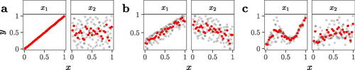
Fig. 1 Scatterplots of $x_k,k=1,2$ against y for three different two-dimensional functions. The red dots show the running mean across 100 simulations. The functions are F1, F2, and F3 in Azzini and Rosati (2022). In (a), y is completely driven by x₁ while x₂ is non-influential. In (b), x₁ is more influential than x₂ given its sharper trend. In (c), x₁ is more influential than x₂ given the presence of larger areas where points are more rarefied. Note that y has been rescaled to (0,1), while the x’s are already in (0,1) being sampled from the unit hypercube.

There are different ways to assess the “uniformity” of a sample. Geometrical criteria such as maximin or minimax respectively maximize the minimal distance between all points or minimize the maximal distance between any location in space and all points of the sample (Pronzato 2017). These criteria are notably used in circle packing problems. In contrast, uniformity criteria measure how the spread of points deviates from a uniform spread of points (in the sense of a multi-dimensional uniform distribution): taking a subspace of the parameter space $J_x=[\mathbf{0},\mathit{x})$, we count the number of points $N_{s_{[\mathbf{0},\mathit{x})}}$ in the subspace and compare it to the total number of the points N_s of the sample. The resulting value is subtracted by the volume of the subspace ${\text{Vol}}_{[\mathbf{0},\mathit{x})}$, (3) $$\left|\frac{N_{s_{[\mathbf{0},\mathit{x})}}}{N_s}-{\text{Vol}}_{[\mathbf{0},\mathit{x})}\right|.$$(3)

The resulting quantity is known as the discrepancy at point x. Notice that with this description, the origin of the domain (${[0]}^d$) is part of every subspace.

Several measures calculate the discrepancy over the whole domain, assumed to be the unit hypercube. Fang, Li, and Sudjianto (2006) proposed seven criteria to assess the quality of discrepancy measures, which we reproduce in Box 1.

Box 1. Fang, Li, and Sudjianto’s (2006) quality criteria for discrepancy measures.

1. They should be invariant under permuting factors and/or runs.

2. They should be invariant under coordinate rotation.

3. They should measure not only uniformity of the hypercube, but also of any sub-projections.

4. They should have some geometric meaning.

5. They should be easy to compute.

6. They should satisfy the Koksma-Hlawka inequality.

7. They should be consistent with other criteria in experimental design, such as the aforementioned distance criteria.

As for criteria 6 in Box 1, the Koksma-Hlawka inequality reads as (4) $$ϵ=\left|E(\mathit{y})-\overline{\mathit{y}}({\text{Vol}}_{[\mathbf{0},\mathit{x})})\right|\le V(f)D^{*},$$(4) where $E(\mathit{y})$ is the true mean of y, $\overline{\mathit{y}}({\text{Vol}}_{[0,\mathit{x})}),$ is the sample mean and V(f) is the total variation of f in the sense of Hardy and Krause (Fang, Li, and Sudjianto 2006). Hence, averaging a function over samples of points with a low discrepancy would achieve a lower integration error as compared to a random sample [also called Monte Carlo (MC) sampling]. Quasi-Monte Carlo (QMC) methods are designed with that problem in mind. For well behaved functions, they typically achieve an integration error close to $O(N_s^{-1})$. There is an extensive body of literature covering methods to create a sample with a low discrepancy. Notably, the low discrepancy sequence of Sobol’ (1967) is one of the most widely used methods and its randomized version nearly achieves a convergence rate of $O(N_s^{-3/2})$ (Owen 2021).

On the matter of discrepancy measures, the L_p-discrepancy measure (Fang et al. 2018), for instance, takes the average of all discrepancies, as (5) $$D_p={\left\{\int {\left|\frac{N_{s_{[\mathbf{0},\mathit{x})}}}{N_s}-{\text{Vol}}_{[\mathbf{0},\mathit{x})}\right|}^p d\mathit{x}\right\}}^{1/p}.$$(5)

When $p\to \infty$, the measure is known as the “star discrepancy,” which corresponds to the Kolmogorov-Smirnov goodness-of-fit statistic (Fang et al. 2018), (6) $$D^{*}=\underset{x\in \mathbf{X}}{\mathrm{\text{sup}}}\left|\frac{N_{s_{[\mathbf{0},\mathit{x})}}}{n}-{\text{Vol}}_{[\mathbf{0},\mathit{x})}\right|.$$(6)

When p = 2, the measure is known as the “star L₂ discrepancy” (Warnock 1972), which corresponds to the Cramér-Von Mises goodness-of-fit statistic (Fang et al. 2018). Its analytical formulation reads as (7) $$\begin{array}{c}S{L}^2({\mathbf{X}}_d^{N_s})=3^{-d}-\frac{2^{1-d}}{N_s}\sum _{i=1}^{N_s}\prod _{k=1}^d\left[1-{(x_k^{(i)})}^2\right]\\ \hspace{1em}+\frac{1}{N_s{}^2}\sum _{i=1}^{N_s}\sum _{j=1}^{N_s}\prod _{k=1}^d\left[1‐\mathrm{\text{max}}(x_k^{(i)},x_k^{(j)})\right].\end{array}$$(7)

The “modified discrepancy” M² slightly varies the “star L₂ discrepancy” (Franco 2008), and reads as (8) $$\begin{array}{c}{M}^2({\mathbf{X}}_d^{N_s})={\left(\frac{4}{3}\right)}^d-\frac{2^{1-d}}{N_s}\sum _{i=1}^{N_s}\prod _{k=1}^d\left[3-{(x_k^{(i)})}^2\right]\\ +\frac{1}{N_s{}^2}\sum _{i=1}^{N_s}\sum _{j=1}^{N_s}\prod _{k=1}^d\left[2‐\mathrm{\text{max}}(x_k^{(i)},x_k^{(j)})\right].\end{array}$$(8)

Equations (5)–(8) do not satisfy the quality criteria listed in Box 1 as they lack sensitivity, vary after rotation and consider the origin to have a special role. To mitigate these issues, some modified formulations of the L₂-discrepancy have been proposed. As we shall see, these methods treat the corners of the hypercube differently. The “centered discrepancy” C², for instance, does not use the origin of the domain when selecting samples to create the volumes, but the closest corner points of the domain to J_x (Hickernell 1998a), as (9) $$\begin{array}{c}{C}^2({\mathbf{X}}_d^{N_s})={\left(\frac{13}{12}\right)}^d-\frac{2}{N_s}\sum _{i=1}^{N_s}\prod _{k=1}^d(1+\frac{1}{2}|x_k^{(i)}-0.5|\\ -\frac{1}{2}|x_k^{(i)}-0.5{|}^2)\\ +\frac{1}{N_s^2}\sum _{i,j=1}^{N_s}\prod _{k=1}^d(1+\frac{1}{2}|x_k^{(i)}-0.5|+\frac{1}{2}|x_k^{(j)}-0.5|\\ -\frac{1}{2}|x_k^{(i)}-x_k^{(j)}|).\end{array}$$(9)

The “symmetric” discrepancy S² is a variation of the centered discrepancy that accounts for the symmetric volume of J_x (Hickernell 1998a): (10) $$\begin{array}{c}{S}^2({\mathbf{X}}_d^{N_s})={\left(\frac{4}{3}\right)}^d-\frac{2}{N_s}\sum _{i=1}^{N_s}\prod _{k=1}^d\left(1+2x_k^{(i)}-2{\left(x_k^{(i)}\right)}^2\right)\\ +\frac{2^d}{N_s^2}\sum _{i,j=1}^{N_s}\prod _{k=1}^d\left(1-|x_k^{(i)}-x_k^{(j)}|\right).\end{array}$$(10)

The “wraparound discrepancy” WD², on the other hand, does not use any corners nor the origin [hence it is also called “unanchored discrepancy”; see Hickernell (1998b)], (11) $$\begin{array}{c}W{D}^2({\mathbf{X}}_d^{N_s})=-{\left(\frac{4}{3}\right)}^d\\ +\frac{1}{N_s^2}\sum _{i,j=1}^{N_s}\prod _{k=1}^d\left(\frac{3}{2}-|x_k^{(i)}-x_k^{(j)}|+|x_k^{(i)}-x_k^{(j)}{|}^2\right).\end{array}$$(11)

The centered discrepancy C² and the wraparound discrepancy WD² are the most commonly used formulations nowadays. As per numerical complexity, these equations have a complexity of $O(N_s^{2}d)$.

2.2 An Ersatz Discrepancy

The discrepancies presented in (5)–(11) are state-of-the-art measures used in the design of computer experiments, requiring statistical training to understand. They are also computationally complex due to their reliance on column-wise and row-wise loops, which limits their scalability for larger sample sizes and higher-dimensional settings. Here, we propose an ersatz discrepancy (S-ersatz hereafter) that addresses these issues and leverages the link between scatterplots, discrepancy, and sensitivity discussed in Section 2.1.

We suggest to split the ${\mathit{x}}_k$, y plane into a uniform grid formed by $\lceil \sqrt{N_s}\rceil \times \lceil \sqrt{N_s}\rceil$ cells, where $\lceil .\rceil$ stands for the ceiling function, and calculate the ratio between the number of cells with points (N_P) and the total number of cells (N_T). Mathematically, this translates into (12) $$S_{\text{ersatz}}=\frac{N_P}{N_T}.$$(12)

Let us now define N_x and N_y as the number of cells along the x- (y-) axis of the grid, and $n_k^{(i)}$ as the number of points in the cell at the intersection of the ith row and the kth column. Based on the properties of a uniform grid, we can also write (13) $$\begin{array}{c}{N}_x=N_y=\lceil \sqrt{N_s}\rceil \hfill \\ N_T=N_x{N}_y\hfill \\ N_P=\sum _{i=1}^{N_x}\sum _{k=1}^{N_y}\mathbb{I}[n_k^{(i)}>0]\hfill \end{array}$$(13) where $\mathbb{I}(.)$ is the indicator function which evaluates to 1 if the condition inside the parentheses is true and 0 otherwise. Hence, (14) $$S_{\text{ersatz}}=\frac{\sum _{i=1}^{N_x}\sum _{k=1}^{N_y}\mathbb{I}[n_k^{(i)}>0]}{N_x{N}_y}.$$(14)

Algorithm 1

The S-ersatz of discrepancy.

1: Calculate the number of cells along the x and y axes of the grid:

2: $$\hspace{1em}{N}_x=N_y=\lceil \sqrt{N_s}\rceil$$

3: Calculate the total number of cells in the grid:

4: $$\hspace{1em}{N}_T=N_x·N_y$$

5: Initialize a variable N_P to 0 ⊳ Count of cells with points

6: for i = 1 to N_x do

7: for k = 1 to N_y do

8: if $N_p(i,k)>0$ then ⊳ Using the indicator function

9: Increment N_P by 1

10: end if

11: end for

12: end for

13: Calculate the ersatz score $S_{\text{ersatz}}$:

14: $$\hspace{1em}{S}_{\text{ersatz}}=\frac{N_P}{N_T}$$

We also provide an algorithmic description of (14) (Algorithm 1). The S-ersatz value thus informs on the fraction of cells that are populated by at least one point: the closer this value is to 1, the more the design approaches a uniform distribution, and the less influential ${\mathit{x}}_k$ is.

Note that the S-ersatz is very close to the general definition of the discrepancy, but differs from previous discrepancy measures in the following features:

1. S-ersatz counts 1 for a cell containing a point and 0 if not, in contrast to the conventional method that calculates the ratio of points to samples in each cell. This results in exact upper and lower bounds: under Quasi-Monte Carlo (QMC) sampling, S-ersatz $\in [1/N_s,1]$, whereas under random sampling, S-ersatz $\in [1/N_s,0.63]$ (proof provided below). Other methods lack straightforward lower bound expressions that cover all combinations of sample sizes and dimensions.

2. Cells are intentionally pre-defined as a uniform grid, corresponding to “property A” described by Sobol’ (1976). “Property A” for a low-discrepancy sequence implies that within any binary segment of the n-dimensional sequence of length $2^{N_s}$, there is precisely one point in each $2^{N_s}$ hyper-octant resulting from subdividing the unit hypercube along its length extensions into halves (Kucherenko, Albrecht, and Saltelli 2015). This property is fundamental in designing certain QMC methods, such as the Sobol’ low-discrepancy sequence.

3. Larger values signify superior uniform properties. For (5)–(11), smaller values are preferable, as they indicate a smaller difference between the distribution of sampling points and a distribution with an equal proportion of points in each explored sub-region of the unit hypercube.

We graphically represent our approach in Figure 2 for both random (a) and quasi-random (b) numbers [Quasi-Monte Carlo (QMC), using the low discrepancy sequence of Sobol’]. The latter are known to outperform the former in sampling the unit hypercube by leaving smaller unexplored volumes. This means that a design with QMC should display larger S-ersatz values than a design based on random numbers. For $N_s=2^2$ (first column), the plane is partitioned into four cells given that $\lceil \sqrt{N_s}\rceil \times \lceil \sqrt{N_s}\rceil =4$. For $N_s=2^b,b=4,6$ (second and third columns), the plane is partitioned into 16 and 64 cells, respectively. The ratio of sampled cells to the total number of cells is $3/4=0.75,11/16=0.68$ and $40/64=0.62$ in a), and $3/4=0.75,12/16=0.75$ and $59/64=0.92$ in b). The behavior of the S-ersatz therefore nicely matches the well-known capacity of quasi-random sequences in covering the domain of interest more evenly and quicker than random numbers (Figure 2(c)).

Fig. 2 The S-ersatz discrepancy. (a) and (b) show planes with sampling points produced using random and QMC (Sobol’ sequence), respectively, for a total sample size of $N_s=2^b,b=2,4,6$. (c) Evolution of the S-ersatz through different N_s .

Figure 2 also indicates that the S-ersatz upper bound for non-influential parameters sampled with QRN approaches 1, while with random numbers, it stabilizes at around $\sim 0.63$. This is because, on average, if we randomly sample n cells with n sampling points, the fraction of cells with at least one point would equal $1-\frac{1}{e}=0.6321206$.

The proof is as follows: let us define the probability of a specific grid cell remaining non-sampled when n points are allocated to n grid cells as ${(1-\frac{1}{n})}^n$. In consequence, and using the concept of complementary probabilities, the probability of a sampled grid cell can be defined as $1-{(1-\frac{1}{n})}^n$, with the average number of cells sampled at least one time denoted as $n\left[1-{(1-\frac{1}{n})}^n\right]$. With n approaching infinity, we have $\underset{n\to \infty }{\mathrm{\text{lim}}}{(1-\frac{1}{n})}^n=e^{-1}=\frac{1}{e}$. It follows that the average number of cells with at least one sampling point is $n\left(1-\frac{1}{e}\right)$, and hence the fraction of cells with at least one sampling point is $\frac{n\left(1-\frac{1}{e}\right)}{n}=1-\frac{1}{e}=0.6321206$.

If we compare our S-ersatz measure with Fang, Li, and Sudjianto’s (2006) quality criteria for discrepancy measures, we see that it displays all properties except number 3 (Box 1):

1,2. It is invariant under rotation and ordering, meaning that changing the order or rotating the space only alters the positions of the subdividing cells, with the respective fractions and global metric remaining unaffected. It is also an unanchored discrepancy, as the origin and corners of the hypercube do not play specific roles.

3. The measure indicates the discrepancy for a given sub-projection. Nevertheless, a composite measure can account for all sub-projections.

4. It holds a geometrical meaning, directly linked to the spread of points in the space’s subdivision.

5. It is simple to approach and implement, in contrast to other SA methods such as Sobol’, and it is computationally fast due to low algorithmic complexity.

6,7. S-ersatz’s definition derives from the discrepancy’s definition, satisfying the Koksma-Hlawka inequality. A high value indicates a lower integration error.

Furthermore, as opposed to classical discrepancy measures, both the upper and lower bounds are exactly known. The worst case would place all points in a single cell, while the ideal case would place a point per cell. This implies S-ersatz $\in [1/N_s,1]$. Other methods do not have simple expressions for their lower bounds which work for all combinations of number of samples and dimensions.

2.3 A Sensitivity Analysis Setting

To explore the extent to which the concept of discrepancy is apt to distinguish influential from non-influential inputs, we benchmark the performance of (7)–(11) and of the S-ersatz (Algorithm 1) in a GSA setting. Specifically, we assess how well each discrepancy measure ranks the most influential parameters, that is, those that convey the most uncertainty to the model output. While the number of influential parameters varies based on the model’s functional form, GSA practitioners generally observe that a small fraction of model inputs typically drives most output variations. This reflects the Pareto principle, where 20% of inputs account for 80% of effects. Consequently, most practitioners focus on identifying only the top-ranked inputs (Sheikholeslami et al. 2019).

As a yardstick of quality, we compare the ranking produced by each discrepancy measure against the ranking produced by Jansen’s (1999) estimator, one of the most accurate variance-based total-order estimators (Saltelli et al. 2010; Puy et al. 2022). Total-order estimators measure the proportion of variance conveyed to y by the first-order effect of x_k jointly with its interactions with all the other parameters (Homma and Saltelli 1996). The total-order effect is computed as follows: (15) $$\begin{array}{c}{T}_k=1-\frac{V_{{\mathit{x}}_{\sim k}}[E_{x_k}(y|{\mathit{x}}_{\sim k})]}{V(y)}\\ =\frac{E_{{\mathit{x}}_{\sim k}}[V_{x_k}(y|{\mathit{x}}_{\sim k})]}{V(y)},\end{array}$$(15) where $E(.)$ and $V(.)$ are the mean and the variance operator, respectively, and ${\mathit{x}}_{\sim k}$ denotes all parameters but x_k. We provide Jansen’s (1999) estimator of T_k in (16).

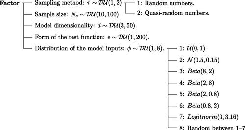
To minimize the influence of the benchmarking design on the results of the analysis, we randomize the main factors that condition the accuracy of sensitivity estimators: the sampling method τ, base sample size N_s, model dimensionality d, form of the test function ϵ and distribution of model inputs $\varphi$ (Becker 2020; Puy et al. 2022). We describe these factors with probability distributions selected to cover a wide range of sensitivity analysis settings, from low-dimensional, computationally inexpensive designs to complex, high-dimensional problems formed by inputs whose uncertainty is described by dissimilar mathematical functions (Figure 3). Although not exhaustive, this approach permits us to go beyond classic benchmarking exercises, which tend to focus on a handful of test functions or just move one design factor at-a-time (Pianosi and Wagener 2015; Azzini and Rosati 2021).

Fig. 3 Tree diagram with the uncertain inputs, their distributions and their levels. $\mathcal{D}\mathcal{U}$ and Logitnorm stand for “discrete uniform” and “log-normal” distribution, respectively.

We first create a $2^9\times 5$ sample matrix using quasi-random numbers (Sobol’ 1967, 1976), where the ith row represents a random combination of $\tau ,N_s,d,ϵ,\varphi$ values and each column is a factor whose uncertainty is described with its selected probability distribution (Figure 3). In the ith row of this matrix we do the following (Saltelli et al. 2010):

1. We construct two sample matrices with the sampling method as defined by ${\tau }^{(i)}$:

   • A $C^{(i)}\times d^{(i)}$ sample matrix, where $C^{(i)}=N_s^{(i)}(d^{(i)}+1)$. This sample matrix is formed by an A matrix and $d^{(i)} {\mathbf{A}}_{B_k}$ matrices. In the latter, all columns come from A except the kth, which comes from B. This sampling design is required to run a sensitivity analysis with the Jansen estimator (Lo Piano et al. 2021b; Puy et al. 2022). We refer to this matrix as the “Jansen matrix”.

   • A $C^{(i)}\times d^{(i)}$ sample matrix formed by an A matrix only given that discrepancy measures do not require a specific sampling design. We match the number of rows of the Jansen matrix to ensure that the comparison between the latter and the discrepancy measures is done on the same total number of model runs. We refer to this matrix as the “Discrepancy matrix”.

2. We define the distribution of each input in these matrices according to the value set by ${\varphi }^{(i)}$ (Figure S1).

3. We run a metafunction rowwise through both the Jansen and the Discrepancy matrices and produce two vectors with the model output, which we refer to as ${\mathit{y}}_J$ and ${\mathit{y}}_D$, respectively. Our metafunction, whose functional form is defined by ${ϵ}^{(i)}$, is based on the Becker (2020) metafunction and randomizes over 13 univariate functions representing common responses in physical systems and in classic SA functions (from cubic, exponential or periodic to sinusoidal, see Figure S2). A detailed explanation of the metafunction can be found in Becker (2020) and in Puy et al. (2022).

4. We use ${\mathit{y}}_J$ to produce a vector with the total-order indices T, calculated with the Jansen (1999) estimator, which reads as follows:

   $\frac{\frac{1}{2N_s}{\sum }_{i=1}^{N_s}{\left[f{(\mathit{A})}^{(i)}-f{({\mathit{A}}_{B_k})}^{(i)}\right]}^2}{V(y)},$ (16)

   where $f(.)$ is the function or model of interest and V(y) the unconditional variance of the model output y. We also use ${\mathit{y}}_D$ to produce seven vectors with the discrepancy values D, one vector for each of the seven discrepancy measures tested.

5. We rank-transform T and D using Savage scores, which emphasize and downplay top and low ranks, respectively (Iman and Conover 1987; Savage 1956). Savage scores are computed by summing the reciprocals of the ranks assigned to a specific element and all the elements below it in a ranked set. Mathematically, if S_s represents the Savage score, and r is the rank assigned to the kth element in a vector of length d, the Savage score is given by the formula

   $S_s={\sum }_{r=k}^d\frac{1}{r}$ (17)

   where r is the rank assigned to the kth element of a vector of length d. For example, if you have a vector $\mathit{x}=(x_1,x_2,x_3)$ where $x_1>x_2>x_3$, the Savage scores would be $S_{s_1}=1+\frac{1}{2}+\frac{1}{3},S_{s_2}=\frac{1}{2}+\frac{1}{3}$, and $S_{s_3}=\frac{1}{3}$.

To check how well discrepancy measures match the ranks produced with the Jansen estimator, we calculate for each discrepancy measure the Pearson correlation between T and D, which we denote as r.

3 Results

3.1 Discrepancy Measures for Sensitivity Analysis

Figure 4(a) presents the results of the analysis in a non-orthogonal domain given that the total number of model runs C is a function of the sample size N_s and the function dimensionality d (Point 1 in Section 2.3). We observe that the symmetric (S²), the centered (C²), the wraparound (WD²) and the S-ersatz present consistently high r values throughout most of the domain investigated, with lower values concentrating largely on the leftmost part of the domain (characterized by simulations with low sample sizes and increasing dimensionality). In contrast, no discernible pattern is visible for the star, L2, centered (C²) or modified (M²) measures, which comparatively present a much larger number of low and negative r values (Figure 4(a)).

Fig. 4 Results of the benchmarking. (a) Distribution of the Pearson correlation r between the Savage scores-transformed ranks yielded by each discrepancy measure and the Savage scores-transformed ranks produced by the Jansen (1999) estimator. Each dot is a simulation that randomizes the sample size N_s, the dimensionality d, the underlying probability distributions $\varphi$, the sampling method τ and the functional form of the metafunction ϵ. The x-axis shows the total cost of the analysis C (the number of model runs), for $C=N_s(d+1)$, and hence the non-orthogonality of the sampling domain. The total number of simulations is 2⁹. (b) Density plots of r values. (c) Tile plot showing the p-values of a pairwise Mood test on medians. (d) Hierarchical clustering.

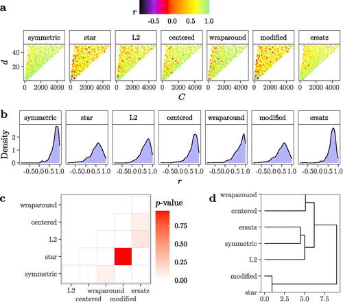
Overall, the distribution of r values is left-skewed for all discrepancy measures. This suggests that they are able to properly approximate the Savage-transformed ranks produced by the Jansen estimator in a non-negligible number of SA settings. According to median values, the discrepancy measure that better matches the Jansen Savage-transformed ranks is the symmetric (S²) (r = 0.81), followed by the wraparound (WD²) (r = 0.78) and the centered (C²) (r = 0.74). The S-ersatz also displays a good performance (r = 0.72), and its spread is as small as that of the symmetric (S²) (Figure 4(b)).

To check whether these median r values come from different distributions, we conduct a pairwise Mood test on medians with corrections for multiple testing and set the probability of a Type I error at $\alpha =0.05$. The pairwise Mood test on medians is a nonparametric test that compares the medians of several independent continuous distributions (Mood, Graybill, and Boes 2007).

We cannot reject the null hypothesis of a difference in medians between the wraparound (WD²) and the symmetric (S²), between the modified (M²) and the star (SL²), or between the ersatz, the L2 and the centered measure (C²) (Figure 4(c)). A hierarchical cluster analysis suggests that the difference in the distribution of r values is mainly between two groups: the group formed by the modified (M²) and the star, and the group formed by all the rest. The star and the modified (M²) discrepancy present the most similar distributions, followed by the S-ersatz and the symmetric (S²) discrepancy (Figure 4(d)).

The capacity of discrepancy measures in matching the Savage-transformed ranks of the Jansen estimator seems to be mostly determined by high-order interactions between the benchmark factors selected in our analysis (Figure 3). The model dimensionality (d) and the base sample size (N_s) are the only factors with a small but still discernible effect on the accuracy of discrepancy measures, especially on the S-ersatz: higher dimensionalities and larger sample sizes tend to respectively diminish and increase their performance (Figure 5). Interestingly, the variability in the performance of discrepancy measures does not seem to be critically determined by the functional form of the model (ϵ), the underlying distribution ($\varphi$) or the sampling method used to design the sample matrix (τ).

Fig. 5 Scatterplot of x_k against r (the Pearson correlation) for each discrepancy measure. The red hexbins display simulations where r < 0. The number of simulations in each facet is $N_s=2^9$.

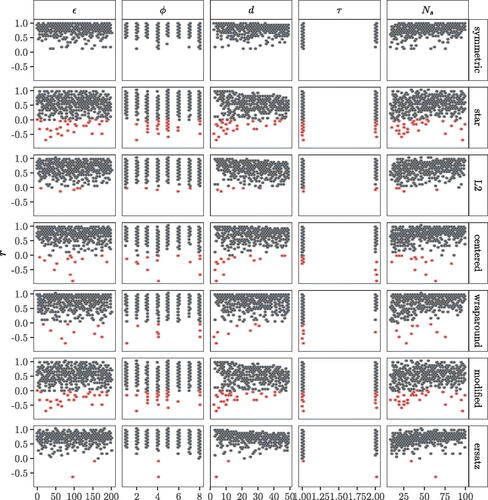
As displayed in Figures 4–5, some simulations yield r < 0. To explore the reasons underlying this rank reversal, we plot all simulations where at least one discrepancy measure yielded r < 0 and cross-check the other r values. We observe that the production of negative r values is measure-specific: in the same simulation some discrepancy measures yielded r < 0 while others produced very high r values and hence accurately matched the rankings of the Jansen estimator (Figures S4–S13). This indicates that certain discrepancy measures, especially the modified (M²) and the star, may be more volatile than the rest when used in an SA setting.

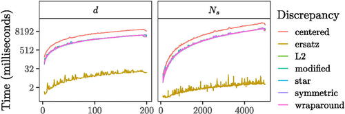
3.2 Computational Complexity

The numerical efficiency of a sensitivity analysis method (how much time it requires to run its algorithmic implementation) is an important property to take into account when deciding which SA approach to use. If the model of interest is already computationally burdensome, the large sample size needed to compute Sobol’ indices or the extra computational strain added by a demanding discrepancy measure may make the implementation of the latter unfeasible. To pinpoint the computational requirements of discrepancy measures, we calculate the time it takes to evaluate each expression with the R package microbenchmark (Mersmann 2021), which uses sub-millisecond accurate timing functions. We use the implementations of (7)–(11) in the R package sensitivity (Iooss et al. 2022), which are written in C++. Our implementation of the S-ersatz algorithm uses base R language (Puy 2022). To gain robust insights into the time complexity of all these discrepancy measures, we explore their efficiency through a wide range of sample sizes N_s (100–5000) and dimensionalities d (3–100), which we treat as random factors following the approach described in Section 2.3. The results, which are presented in Figure 6, match the expected numerical complexity of the different discrepancy measures, $O(N_s^{2}d)$, and of the S-ersatz, $O(N_{s}d)$.

Fig. 6 Time complexity of discrepancy measures. In the d facet N_s = 500, while in the N_s facet, d = 5.

4 Discussion and Conclusions

SA is a key method to ensure the quality of model-based inferences and promote responsible modeling (Saltelli et al. 2020; Saltelli and Di Fiore 2023). Here we investigate the utility of using discrepancy measures as tools to assess the sensitivity of a model output to its input uncertainties. Our contribution can be summarized in three key aspects:

1. We try to make SA more accessible to the non-specialist by linking the sensitivity of a given input to this input’s capacity to leave “holes” in the input-output scatterplot. The use of discrepancy measures as a SA method thus permits an easy explanation as to why a factor is identified as more influential than another: for instance, x₁ is more influential than x₂ when the scatterplot of x₁ against y displays a more discernible shape and more “holes” than the scatterplot of x₂ against y. The capacity to be translated into comprehensive language is regarded as a desirable property of a good SA method (Saltelli et al. 2008), and this feature is also shared by variance-based methods: the first-order index (S_i) says that x₁ is more important than x₂ when fixing x₁ leads on average to a greater reduction in the output variance than fixing x₂. As for the total-order index (T_i), it says that x₁ is more important than x₂ when fixing all factors but x₁ leaves on average a greater residual variance than doing the same on x₂.

2. We present numerical evidence that discrepancy is an effective proxy for Sobol’s total-order sensitivity index, whose use is considered best practice in variance-based SA (Homma and Saltelli 1996; Saltelli et al. 2008). We cannot compare the discrepancy measure against the theoretical, analytic values of the Sobol’ indices as this would limit our analysis to those functions for which such a solution exists [a library of such functions is available in Kucherenko et al. (2011)]. Instead, our analysis randomly generates test functions over broad ranges of linearity and additivity to ensure that our results remain independent of the choice of the test function. Such approach also aligns better with current SA practices: most of the time the effects of nonlinearities and non-additivities in models are unknown to analysts before running the model, including the “true” Sobol’ indices. Overall, our approach might have greater appeal for those users that have less familiarity with statistical or mathematical concepts such as ANOVA of functional decompositions. The results might also be easier to communicate by the analyst to the owner of the problem for those cases where the two are not the same person.

   Finally, it is also worth stating that, although the S-ersatz is able to capture effects given by interactions like the total-order index, it can not treat group (set) effects as this would imply to plot y along the sorted set. A future exploration of this topic could be attempted using Fourier decompositions as in the sensitivity analysis method known as FAST (Saltelli, Tarantola, and Chan 1999).

3. We introduce an ersatz discrepancy whose behavior in an SA setting approximates the best discrepancy measures at a much reduced computational cost. We observe the existence of two groups: (a) the group formed by the wraparound, the centered, the symmetric, the L2 and the S-ersatz, and (b) the group formed by the modified and the star discrepancies. The second group matches the behavior of the Jansen estimator worse than the first group because both the modified and the star discrepancy give the origin of the domain (${[0]}^d$) a special meaning: points further away from the origin affect less the measures. As for discrepancy measures in the first group, their behavior is similar because they also treat the origin and corner points in the same way. Their differences due to the dimensionality do not play an important role here given our focus on 2D sub-projections.

   Our results suggest that the symmetric is the most robust discrepancy measure for SA, and that it should be prioritized over the other measures if the practitioner is interested in a discrepancy-based SA. However, its numerical complexity might make it computationally unaffordable for high-dimensional models or if several model runs are required. In those settings, the S-ersatz offers a much lighter and efficient alternative without trading too much in accuracy. If the correlation between the Jansen and the symmetric equals r = 0.81 and the correlation between the Jansen and the S-ersatz equals r = 0.72, this implies a 9% accuracy loss if using the latter.

Regardless of whether the symmetric or the S-ersatz measure is selected, it is crucial to ensure the quality of the sampling by using randomized QMC methods like Sobol’ low-discrepancy sequences, which ensure uniformity on sub-projections (Sobol’ 1967; Kucherenko, Albrecht, and Saltelli 2015). It is important to have a uniform distribution on the sample axis because we are constructing 2D sub-projections between x_k and y and because the S-ersatz discretizes the projected space into boxes. It is not sufficient to only have good sub-projection on 1D sub-projections as the output is still determined by the sample values in all dimensions.

The use of discrepancy measures in an SA setting can be extended to higher dimensions to appraise high order interactions. Both the centered and the wraparound discrepancy, however, are known to have shortcomings with regards to dimensionality: the centered suffers from the curse of dimensionality, whereas the wraparound is not sensitive to a shift of dimension (Zhou, Fang, and Ning 2013; Fang et al. 2018). Our results may therefore change should we increase the sub-projections’ dimensionality. Recently, some work has been done to combine the complementary benefits of both the centered and the wraparound discrepancy into a single measure: the mixture discrepancy MD² (see Zhou, Fang, and Ning 2013). This method could also prove to be efficient here as it should give a more uniform importance to every part of the domain. Finally, and given that our study has focused on scalar outputs only, further work can be directed to explore how discrepancy measures perform as SA tools under multi-variate outputs. In current SA practices, the most appropriate method appears to be contingent upon the nature of the output, be it a map, a time-series or a multi-variate result (Constantine 2015; Razavi et al. 2021).

Supplementary Materials

In the online Supplementary Materials we include Figures S1–S13, which provide additional information about the metafunction used in Section 2.3 and the results presented in Section 3.1. In the zip file we include the R code to reproduce our results and all the figures of the manuscript, as well as a README file with instructions on how to execute the code. The R code can also be retrieved from Puy (2022). Finally, a function to calculate the S-ersatz is available in the R package sensobol (Puy et al. 2022) and the Python library SALib (Herman and Usher 2017).

Disclosure Statement

No potential conflict of interest was reported by the author(s).

Additional information

Funding

This work was funded by UK Research and Innovation (UKRI) under the UK government’s Horizon Europe funding guarantee (project DAWN, PI Arnald Puy, EP/Y02463X/1). Andrea Saltelli acknowledges the i4Driving project (Horizon 2020, grant agreement ID 101076165).

References

- Azzini, I., and Rosati, R. (2021), “Sobol’ Main Effect Index: An Innovative Algorithm (IA) Using Dynamic Adaptive Variances,” Reliability Engineering & System Safety, 213, 107647. DOI: 10.1016/j.ress.2021.107647.
- ———(2022), “A Function Dataset for Benchmarking in Sensitivity Analysis,” Data in Brief, 42, 108071. DOI: 10.1016/j.dib.2022.108071.
- Barr, J., and Rabitz, H. (2022), “A Generalized Kernel Method for Global Sensitivity Analysis,” SIAM/ASA Journal on Uncertainty Quantification, 10, 27–54. DOI: 10.1137/20M1354829.
- ———(2023), “Kernel-based Global Sensitivity Analysis Obtained from A Single Data Set,” Reliability Engineering & System Safety, 235, 109173. DOI: 10.1016/j.ress.2023.109173.
- Becker, W. (2020), “Metafunctions for Benchmarking in Sensitivity Analysis,” Reliability Engineering and System Safety, 204, 107189. DOI: 10.1016/j.ress.2020.107189.
- Borgonovo, E. (2007), “A New Uncertainty Importance Measure,” Reliability Engineering and System Safety, 92, 771–784. DOI: 10.1016/j.ress.2006.04.015.
- Borgonovo, E., and Plischke, E. (2016), “Sensitivity Analysis: A Review of Recent Advances,” European Journal of Operational Research, 248, 869–887. DOI: 10.1016/j.ejor.2015.06.032.
- Constantine, P. G. (2015), Active Subspaces: Emerging Ideas for Dimension Reduction in Parameter Studies. SIAM Spotlights 2, 100 pp., Philadelphia: Society for Industrial and Applied Mathematics.
- European Commission. (2023), “Better Regulation Toolbox.” Available at https://ec.europa.eu/info/law/law-making-process/planning-and-proposing-law/better-regulation-why-and-how/better-regulation-guidelines-and-toolbox_en, November 25. Accessed 21/01/2024.
- Fang, K.-T., Li, R., and Sudjianto, A. (2006), Design and Modeling for Computer Experiments, London: Chapman & Hall.
- Fang, K.-T., Liu, M.-Q., Qin, H., and Zhou, Y.-D. (2018), Theory and Application of Uniform Experimental Designs (Vol. 221). Lecture Notes in Statistics. Singapore: Springer. DOI: 10.1007/978-981-13-2041-5.
- Franco, J. (2008), “Planification d’Expériences numériques en phase exploratoire pourla simulation des phénomènes complexes,” Ecole Nationale Supérieure des Mines Saint-Etienne.
- Herman, J., and Usher, W. (2017), “SALib: An open-source Python library for Sensitivity Analysis,” The Journal of Open Source Software, 2. DOI: 10.21105/joss.00097.
- Hickernell, F. J. (1998a), “A Generalized Discrepancy and Quadrature Error Bound,” Mathematics of Computation, 67, 299–322. DOI: 10.1090/S0025-5718-98-00894-1.
- ———(1998b), “Lattice Rules: How Well Do They Measure Up?” in Random and Quasi-Random Point Sets, eds. P. Hellekalek and G. Larcher, pp. 109–166, New York: Springer. DOI: 10.1007/978-1-4612-1702-2_3.
- Homma, T., and Saltelli, A. (1996), “Importance Measures in Global Sensitivity Analysis of Nonlinear Models,” Reliability Engineering & System Safety, 52, 1–17. DOI: 10.1016/0951-8320(96)00002-6.
- Iman, R. L., and Conover, W. J. (1987), “A Measure of Top-Down Correlation,” Techno Metrics, 29, 351–357. DOI: 10.2307/1269344.
- Iooss, B., Da Veiga, S., Janon, A., Pujol, G., with contributions from Broto, B., Boumhaout, K., Delage, T., El Amri, R., Fruth, J., Gilquin, L., Guillaume, J., Herin, M., Il Idrissi, M., Le Gratiet, L., Lemaitre, P., Marrel, A., Meynaoui, A., Nelson, B. L., Monari, F., Oomen, R., Rakovec, O., Ramos, B., Roustant, O., Sarazin, G., Song, E., Staum, J., Sueur, R., Touati, T., Verges, V., and Weber, F. (2022), “Sensitivity: Global Sensitivity Analysis of Model Outputs,” manual.
- Jansen, M. (1999), “Analysis of Variance Designs for Model Output,” Computer Physics Communications, 117, 35–43. DOI: 10.1016/S0010-4655(98)00154-4.
- Kucherenko, S., Albrecht, D., and Saltelli, A. (2015), “Exploring Multi-Dimensional Spaces: A Comparison of Latin Hypercube and Quasi Monte Carlo Sampling Techniques,” DOI: 10.48550/ARXIV.1505.02350.
- Kucherenko, S., Feil, B., Shah, N., and Mauntz, W. (2011), “The Identification of Model Effective Dimensions Using Global Sensitivity Analysis,” Reliability Engineering & System Safety, 96, 440–449. DOI: 10.1016/j.ress.2010.11.003.
- Lo Piano, S., Ferretti, F., Puy, A., Albrecht, D., and Saltelli, A. (2021), “Variance-based Sensitivity Analysis: The Quest for Better Estimators and Designs between Explorativity and Economy,” Reliability Engineering & System Safety, 206, 107300. DOI: 10.1016/j.ress.2020.107300.
- Mersmann, O. (2021), microbenchmark: Accurate Timing Functions. Manual.
- Mood, A. M., Graybill, F. A., and Boes, D. C. (2007), Introduction to the Theory of Statistics (3rd ed), McGraw-Hill Series in Probability and Statistics, 564 pp., New York: McGraw-Hill.
- Owen, A. B. (2014), “Sobol Indices and Shapley Value,” SIAM-ASA Journal on Uncertainty Quantification, 2, 245–251. DOI: 10.1137/130936233.
- ———(2021), On Dropping the First Sobol’ Point, arXiv: 2008.08051 [math.NA].
- Pianosi, F., and Wagener, T. (2015), “A Simple and Efficient Method for Global Sensitivity Analysis based on Cumulative Distribution Functions,” Environmental Modelling and Software, 67, 1–11. DOI: 10.1016/j.envsoft.2015.01.004.
- Pianosi, F., Beven, K., Freer, J., Hall, J. W., Rougier, J., Stephenson, D. B., and Wagener, T. (2016), “Sensitivity Analysis of Environmental Models: A Systematic Review with Practical Workflow,” Environmental Modelling and Software, 79, 214–232. DOI: 10.1016/j.envsoft.2016.02.008.
- Pronzato, L. (2017), “Minimax and Maximin Space-Filling Designs: Some Properties and Methods for Construction,” Journal de la Société Française de Statistique, 158, 7–36.
- Puy, A. (2022), “Code of Discrepancy Measures for Global Sensitivity Analysis,” Zenodo. DOI: 10.5281/zenodo.6760348.
- Puy, A., Becker, W., Lo Piano, S., and Saltelli, A. (2022), “A Comprehensive Comparison of Total-Order Estimators for Global Sensitivity Analysis,” International Journal for Uncertainty Quantification, 12, 1–18. DOI: 10.1615/Int.J.UncertaintyQuantification.2021038133.
- Puy, A., Lo Piano, S., and Saltelli, A. (2020), “A Sensitivity Analysis of the PAWN Sensitivity Index,” Environmental Modelling & Software, 127, 104679. DOI: 10.1016/j.envsoft.2020.104679.
- Puy, A., Lo Piano, S., Saltelli, A., and Levin, S. A. (2022), “sensobol: an R Package to Compute Variance-based Sensitivity Indices,” Journal of Statistical Software, 102, 1–37. DOI: 10.18637/jss.v102.i05.
- Razavi, S., and Gupta, H. V. (2016), “A New Framework for Comprehensive, Robust, and Efficient Global Sensitivity Analysis: 1. Theory,” Water Resources Research, 52, 423–439. DOI: 10.1002/2015WR017559.
- Razavi, S., Jakeman, A., Saltelli, A., Prieur, C., Iooss, B., Borgonovo, E., Plischke, E., Lo Piano, S., Iwanaga, T., Becker, W., Tarantola, S., Guillaume, J. H. A., Jakeman, J., Gupta, H., Melillo, N., Rabitti, G., Chabridon, V., Duan, Q., Sun, X., Smith, S., Sheikholeslami, R., Hosseini, N., Asadzadeh, M., Puy, A., Kucherenko, S., and Maier, H. R. (2021), “The Future of Sensitivity Analysis: An Essential Discipline for Systems Modeling and Policy Support,” Environmental Modelling & Software, 137, 104954. DOI: 10.1016/j.envsoft.2020.104954.
- Saltelli, A. (2002), “Sensitivity Analysis for Importance Assessment,” Risk Analysis, 22, 579–590. DOI: 10.1111/0272-4332.00040.
- Saltelli, A., Aleksankina, K., Becker, W., Fennell, P., Ferretti, F., Holst, N., Li, S., and Wu, Q. (2019), “Why So Many Published Sensitivity Analyses are False: A Systematic Review of Sensitivity Analysis Practices,” Environmental Modelling and Software, 114, 29–39. DOI: 10.1016/j.envsoft.2019.01.012.
- Saltelli, A., Annoni, P., Azzini, I., Campolongo, F., Ratto, M., and Tarantola, S. (2010), “Variance based Sensitivity Analysis of Model Output. Design and Estimator for the Total Sensitivity Index,” Computer Physics Communications, 181, 259–270. DOI: 10.1016/j.cpc.2009.09.018.
- Saltelli, A., Bammer, G., Bruno, I., Charters, E., Di Fiore, M., Didier, E., Espeland, W. N., Kay, J., Lo Piano, S., Mayo, D., Pielke Jr, R., Portaluri, T., Porter, T. M., Puy, A., Rafols, I., Ravetz, J. R., Reinert, E., Sarewitz, D., Stark, P. B., Stirling, A., van der Sluijs, J., and Vineis, P. (2020), “Five Ways to Ensure that Models Serve Society: A Manifesto,” Nature, 582, 482–484. DOI: 10.1038/d41586-020-01812-9.
- Saltelli, A., and Di Fiore, M., eds. (2023), The Politics of Modelling. Numbers Between Science and Policy, Oxford: Oxford University Press.
- Saltelli, A., Ratto, M., Andres, T., Campolongo, F., Cariboni, J., Gatelli, D., Saisana, M., and Tarantola, S. (2008), Global Sensitivity Analysis. The Primer, Chichester, UK: Wiley. DOI: 10.1002/9780470725184.
- Saltelli, A., Tarantola, S., and Chan, K. P.-S. (1999), “A Quantitative Model-Independent Method for Global Sensitivity Analysis of Model Output,” Technometrics: A Journal of Statistics for the Physical, Chemical, and Engineering Sciences, 41, 39. DOI: 10.2307/1270993.
- Savage, I. R. (1956), “Contributions to the Theory of Rank Order Statistics - The Two Sample Case,” Annals of Mathematical Statistics, 27, 590–615. DOI: 10.1214/aoms/1177728170.
- Sheikholeslami, R., Razavi, S., Gupta, H. V., Becker, W., and Haghnegahdar, A. (2019), “Global Sensitivity Analysis for High-Dimensional Problems: How to Objectively Group Factors and Measure Robustness and Convergence While Reducing Computational Cost,” Environmental Modelling and Software, 111, 282–299. DOI: 10.1016/j.envsoft.2018.09.002.
- Sobol’, I. M. (1967), “On the Distribution of Points in a Cube and the Approximate Evaluation of Integrals,” USSR Computational Mathematics and Mathematical Physics, 7, 86–112. DOI: 10.1016/0041-5553(67)90144-9.
- ———(1976), “Uniformly Distributed Sequences with an Additional Uniform Property,” USSR Computational Mathematics and Mathematical Physics, 16, 236–242. DOI: 10.1016/0041-5553(76)90154-3.
- US Environmental Protection Agency. (2009), Guidance on the Development, Evaluation, and Application of Environmental Models. Office of the Science Advisor, Council for Regulatory Environmental Modeling, pp. 1–99.
- Warnock, T. T. (1972), “Computational Investigations of Low-Discrepancy Point Sets,” in Applications of Number Theory to Numerical Analysis, eds. S. K. Zaremba, pp. 319–343, New York: Academic Press. DOI: 10.1016/B978-0-12-775950-0.50015-7.
- Zhou, Y.-D., Fang, K.-T., and Ning, J.-H. (2013), “Mixture Discrepancy for Quasirandom Point Sets,” Journal of Complexity 29(3):283–301. DOI: 10.1016/j.jco.2012.11.006.