Active sampling: A machine-learning-assisted framework for finite population inference with optimal subsamples

Abstract

Data subsampling has become widely recognized as a tool to overcome computational and economic bottlenecks in analyzing massive datasets. We contribute to the development of adaptive design for estimation of finite population characteristics, using active learning and adaptive importance sampling. We propose an active sampling strategy that iterates between estimation and data collection with optimal subsamples, guided by machine learning predictions on yet unseen data. The method is illustrated on virtual simulation-based safety assessment of advanced driver assistance systems. Substantial performance improvements are demonstrated compared to traditional sampling methods. Supplementary materials for this article are available online.

Keywords:

• active learning
• adaptive importance sampling
• computer simulation experiments
• inverse probability weighting
• optimal design
• traffic safety assessment

Disclaimer

As a service to authors and researchers we are providing this version of an accepted manuscript (AM). Copyediting, typesetting, and review of the resulting proofs will be undertaken on this manuscript before final publication of the Version of Record (VoR). During production and pre-press, errors may be discovered which could affect the content, and all legal disclaimers that apply to the journal relate to these versions also.

1 Introduction

We consider a deterministic computer simulation experiment which for a given input z returns a fixed output y. The input space is assumed to be discrete and the simulation experiment hence characterized by the set of complete input-output pairs ${\{({\mathit{z}}_i,{\mathit{y}}_i)\}}_{i=1}^N$, where N is the size of the experiment. The aim our experiment it to calculate a characteristic(1) $$\theta =h({\mathit{t}}_{\mathit{y}}),\hspace{1em}{\mathit{t}}_{\mathit{y}}=\sum _{i=1}^N{\mathit{y}}_i,$$(1) for some differentiable function $h:{ℝ}^d\to ℝ$ and d-dimensional vector of totals ${\mathit{t}}_{\mathit{y}}$. Examples of such a characteristic include, e.g., a total, mean, ratio, or correlation coefficient. This is also known as a finite population inference problem (Beaumont and Haziza, 2022). We further assume that N is large, as is the computational cost of each single experiment, rendering complete enumeration unfeasible. In such circumstances, researches often resort to subsampling.

Subsampling methods have seen a huge increase in popularity over the past few years across many different areas of statistics. For instance, Ma et al. (2015, 2022) introduced leverage sampling for big data regression, which subsequently inspired similar developments for logistic regression (Wang et al., 2018; Yao and Wang, 2019) generalized linear models (Ai et al., 2021b; Yu et al., 2022), and quantile regression (Ai et al., 2021a; Wang et al., 2021). Similarly, Dai et al. (2022) developed an optimal subsampling method for regression using a minimum energy criterion. Sometimes subsampling is induced by economical rather than computational constraints. In this setting, Imberg et al. (2022) developed an optimal subsampling method for two-phase sampling experiments. A similar measurement-constrained experiment problem was addressed by Zhang et al. (2021) using a sequential subsampling procedure and by Meng et al. (2021) using a space-filling Latin hypercube sampling method.

For computer simulation experiments, subsampling methods using adaptive design for Gaussian process response surface modeling are commonly employed. Together with active learning and Bayesian optimization, this provides a powerful framework for computer experiment emulation (Gramacy and Apley, 2015; Sun et al., 2017; Lei et al., 2021; Lim et al., 2021). Another popular approach is model-free space-filling methods using, e.g., Latin hypercube sampling designs (see, e.g., Cioppa and Lucas, 2007; Zhang et al., 2024; Zhou et al., 2024). Others have utilized methods based on optimal transport, e.g., for kernel density estimation (Zhang et al., 2023). For estimating a simple statistic, such as a mean or ratio, however, importance sampling and adaptive importance sampling remains prominent (Bucher, 1988; Oh and Berger, 1992; Feng et al., 2021). Importance sampling is widely known, easy to implement, and provides consistent estimates under minimal assumptions (Fishman, 1996; Fuller, 2009). Some recent developments include adaptive importance sampling for quantile estimation (Pan et al., 2020) and online monitoring of data streams (Liu et al., 2015; Xian et al., 2018).

There has also been a considerable interest in subsampling and adaptive design in machine learning, particularly in the context of active learning (MacKay, 1992; Cohn, 1996; Settles, 2012). Adaptive importance sampling methods for active learning were developed in, e.g., Bach (2007), Beygelzimer et al. (2009) and Imberg et al. (2020). Active learning has also been utilized for deep learning (Ren et al., 2021), Gaussian processes (Sauer et al., 2023) and adaptive design of experiments (Lookman et al., 2019; Sun et al., 2021), to mention a few.

Returning to the finite population inference problem (1), this is a classical problem in statistics and hence has achieved considerable attention over the years, particularly in the survey sampling literature. Common approaches to estimation include importance sampling methods and/or using estimators that utilize information of known auxiliary variables to improve estimator efficiency (see, e.g., Cassel et al., 1976; Deville and Särndal, 1992; Kott, 2016; Ta et al., 2020). Methods utilizing machine learning in survey sampling have just recently begun to emerge (Breidt and Opsomer, 2017; Kern et al., 2019; McConville and Toth, 2019; Sande and Zhang, 2021). Although there has been a substantial amount of work on subsampling and adaptive design in the statistical literature, there is to our knowledge little done at the intersection of machine learning and adaptive design for the finite population inference problem (1).

Contributions

To fill the gap in adaptive design and machine learning for finite population inference, we propose an active sampling strategy for estimation of finite population characteristics. Our method iterates between estimation and data collection with optimal subsamples, guided by machine learning predictions on yet unseen data. The proposed sampling strategy interpolates in a completely data-driven manner between simple random sampling when no auxiliary information is available and optimal importance sampling as more information is acquired. Consistency and asymptotic normality of the active sampling estimator is established using martingale central limit theory. Methods for variance estimation are proposed and conditions for consistent variance estimation presented.

Outline

The structure of this paper is as follows: We start by presenting a motivating example in crash-causation-based scenario generation for virtual vehicle safety assessment in Section 2. Mathematical preliminaries and notation is introduced in Section 3. In the end of this section we also derive an optimal importance sampling scheme for estimating a finite population characteristic while accounting for uncertainty in the study variables of interest. This is then incorporated in the active sampling algorithm proposed in Section 4. An empirical evaluation on simulated data is conducted in Section 5 and application to virtual vehicle safety assessment in Section 6. Additional theoretical results and proofs are provided in the Supplementary Material.

2 Motivating example

Traffic safety is a problem worldwide (World Health Organization, 2018). Safety systems have been developed to improve traffic safety and have shown the potential to avoid or mitigate crashes. However, when developing both advanced driver assistance systems and automated driving systems, there is a need to assess the impact on safety of the systems before they are on the market. One way to do that is by running virtual simulations comparing the outcome of simulations both with and without a specific system (Seyedi et al., 2021; Leledakis et al., 2021).

We consider a virtual simulation experiment based on a glance-and-deceleration crash-causation model where a driver’s off-road glance behavior and braking profile are represented by discrete (empirical) probability distributions, using a similar setup as in Bärgman et al. (2015) and Lee et al. (2018). The outcome of the simulations is a distribution of impact speeds of all the crashes generated by all combinations of the eyes-off-road glace duration and the maximum deceleration during braking. Here “all combinations” is the problem. Complete enumeration becomes practically unfeasible in high-dimensional (many parameters varied) or high-resolution (many levels per parameter) settings, and subsampling is inevitable.

A small toy example of our problem and illustration of the proposed active sampling method is provided in Figure 1. The figure shows the output of a computer simulation experiment to evaluate the impact speed reduction with an automatic emergency braking system (AEB) compared to a baseline manual driving scenario (without AEB) in a rear-end collision generation. The impact speed and impact speed reduction depend on the maximal deceleration during braking and the driver’s off-road glance duration, i.e., the time the driver of the ’following’ car is looking off-road (e.g., due to distraction). By iteratively learning to predict the response surface of Figure 1 A while running the experiment, an accurate estimate of the overall safety benefit of the AEB system may be obtained by adaptive importance sampling (Figure 1 B). In doing so, computational demands can be substantially reduced compared to complete enumeration.

3 Finite population sampling

We introduce the mathematical framework and notation in Section 3.1, presented in the context of the crash-causation-based scenario generation application outlined above. Traditional methods for sample selection and estimation are reviewed in Section 3.2 and optimal importance sampling schemes discussed in Section 3.3.

3.1 Target characteristic and scope of inference

Assume we are given an index set or dataset $\mathcal{D}$ with N instances or elements $i=1,\dots ,N$. Associated with each element i in $\mathcal{D}$ is a vector $({\mathit{y}}_i,{\mathit{z}}_i)$, where ${\mathit{y}}_i$ is a vector of outcomes or response variables, and ${\mathit{z}}_i$ a vector of design variables and auxiliary variables. We are interested in a characteristic $\theta =h({\mathit{t}}_{\mathit{y}})$ for some differentiable function $h:{ℝ}^d\to ℝ$ and d-dimensional vector of totals ${\mathit{t}}_{\mathit{y}}={\sum }_{i=1}^N{\mathit{y}}_i$.

In the context of crash-causation-based scenario generation, the index set $\mathcal{D}$ represents a collection of N potential simulation scenarios of interest. The response variables ${\mathit{y}}_i$ are outcomes of the simulation, including, e.g., whether a crash occurred or not, impact speed if there was a crash, and impact speed reduction with an advanced driver assistance system compared to some baseline driving scenario. The auxiliary variables ${\mathit{z}}_i$ contain scenario information, such as simulation settings and parameters that are under the control of the investigator, and any additional information that is available without running the actual simulation. Characteristics of interest include, e.g., the mean impact speed reduction and crash avoidance rate with an advanced driver assistance system compared to some baseline driving scenario, when restricted to the relevant set of crashes (Figure 1).

3.2 Unequal probability sampling

In our application, as in many computer simulation experiment applications, running all N simulations of interest to observe the outcomes ${\left\{{\mathit{y}}_i\right\}}_{i=1}^N$ is computationally unfeasible. Hence, we assume that observing complete data is affordable only for a subset $\mathcal{S}\subset \mathcal{D}$ of size n. We consider the case when the subset $\mathcal{S}$ is selected using unequal probability sampling, i.e., by a random mechanism where each instance $i\in \mathcal{D}$ has a strictly positive and possibly unique probability of selection. In this section we also restrict ourselves to non-adaptive designs. We let S_i be the random variable representing the number of times an element i is selected by the sampling mechanism, assuming that sampling may be with replacement. Hence, the subsample $\mathcal{S}$ is the random set given by $\mathcal{S}=\{i\in \mathcal{D}:S_i>0\}$. We will primarily consider multinomial sampling designs but note that the methodology of our paper is applicable also for other designs, such as the Poisson sampling design (Tillé, 2006), with minimal modifications.

In this context, an estimator for the finite population characteristic (1) may be obtained by sample weighting as(2) $$\widehat{\theta }=h({\widehat{\mathit{t}}}_{\mathit{y}}),\hspace{1em}{\widehat{\mathit{t}}}_{\mathit{y}}=\sum _{i\in \mathcal{S}}{S}_i{w}_i{\mathit{y}}_i,$$(2) where $w_i=1/{\mu }_i$ and ${\mu }_i=\mathrm{E}[S_i]$. We note that ${\widehat{\mathit{t}}}_{\mathit{y}}$ is an unbiased estimator of the total ${\mathit{t}}_{\mathit{y}}$ provided that ${\mu }_i>0$ for all $i\in \mathcal{D}$, and furthermore a consistent estimator under general conditions (Hansen and Hurwitz, 1943; Horvitz and Thompson, 1952). Consequently, $\widehat{\theta }$ is a consistent estimator for θ under mild assumptions (see, e.g., Fuller, 2009).

3.3 Optimal importance sampling schemes

When the function h is linear and all $h({\mathit{y}}_i)$ are positive, it is well-known that the optimal sampling scheme for θ in terms of minimizing the variance of the estimator $\widehat{\theta }$ is given by ${\mu }_i\propto h({\mathit{y}}_i)$, in fact producing an estimator with zero variance (Fishman, 1996). In general, one can show that the optimal importance sampling scheme for a characteristic $\theta =h({\mathit{t}}_{\mathit{y}})$ and non-linear function $h(\mathit{u})$ is of the form ${\mu }_i\propto |\nabla h{({\mathit{t}}_{\mathit{y}})}^T{\mathit{y}}_i|$ (Proposition 1). A proof is provided in Section A in the Supplement.

Proposition 1 (Optimal importance sampling scheme, ${\mathit{y}}_i$ known). Let ${\left\{{\mathit{y}}_i\right\}}_{i=1}^N$ befixed. Let ${\left\{m_k\right\}}_{k\ge 1}$ be an increasing sequence of positive integers and ${\mathit{S}}_k=(S_{k1},\dots ,S_{kN})\sim \text{Multinomial}(m_k,\mathit{\pi })$ a corresponding sequence of random vectors. Let ${\widehat{\theta }}_k$ be defined for the $k^{\text{th}}$ random vector ${\mathit{S}}_k$ as in (2). As a function of $\mathit{\pi }=({\pi }_1,\dots ,{\pi }_N)$, the asymptotic mean squared error $\text{AMSE}(\widehat{\theta }):=\underset{k\to \infty }{\lim }\mathrm{E}[m_k{({\widehat{\theta }}_k-\theta )}^2]$ is minimized by (3) $${\pi }_i^{*}=\frac{\sqrt{c_i}}{\sum _{j=1}^N\sqrt{c_j}},\hspace{1em}i=1,\dots ,N,$$(3) with $c_i=|\nabla h{(\mathit{u})}^T{\mathit{y}}_i{|}_{\mathit{u}={\mathit{t}}_{\mathit{y}}}^2$.

We note that the result of Proposition 1 is of limited practical use as it requires all the ${\mathit{y}}_i$’s to be known. Inspired by active learning (Settles, 2012), we introduce in Section 4 an active sampling algorithm that overcomes this limitation through sequential sampling with iterative updates of the estimate for the total ${\mathit{t}}_{\mathit{y}}$ and predictions for the ${\mathit{y}}_i$’s. However, as shown in the experiments in Section 5, naively plugging in the predictions immediately to the importance sampling scheme of Proposition 1 often results in poor performance. Indeed, accounting for prediction error is essential to control the variance of the active sampling estimator. We therefore in Proposition 2 propose an optimal importance sampling scheme to minimize the expected mean squared error of our estimator for θ, treating the unobserved values of the ${\mathit{y}}_i$’s as random variables ${\mathit{Y}}_i$. Integrated with flexible machine learning models, this will be the key ingredient of the active sampling method introduced in Section 4.

Proposition 2 (Optimal importance sampling scheme, ${\mathit{y}}_i$ unknown). Let ${\left\{{\mathit{y}}_i\right\}}_{i=1}^N,{\mathit{t}}_{\mathit{y}}={\sum }_{i=1}^N{\mathit{y}}_i$ and $\theta =h({\mathit{t}}_{\mathit{y}})$ be fixed but unknown constants. Consider, as a proxy for ${\mathit{y}}_i$, a collection of random variables ${\left\{{\mathit{Y}}_i\right\}}_{i=1}^N$ with means $\mathrm{E}[{\mathit{Y}}_i]={\mathit{\eta }}_i$ and finite, positive semi-definite covariance matrices $\mathbf{Cov}({\mathit{Y}}_i)={\mathbf{\Sigma }}_i$. Let m_k, ${\mathit{S}}_k,{\widehat{\theta }}_k$ and $\text{AMSE}(\widehat{\theta })$ be defined as in Proposition 1. Then, the expected asymptotic mean squared error ${\mathrm{E}}_{\mathit{Y}}[\text{AMSE}(\widehat{\theta })]$ is minimized by (3) with $c_i={\left[{(\nabla h{(\mathit{u})}^T{\mathit{\eta }}_i)}^2+\nabla h{(\mathit{u})}^T{\mathbf{\Sigma }}_i\nabla h(\mathit{u})\right]}_{\mathit{u}={\mathit{t}}_{\mathit{y}}}$.

For a proof, see Section A in the Supplement.

4 Active sampling

In this section we propose an active sampling strategy for finite population inference with optimal subsamples using adaptive importance sampling and machine learning. The active sampling algorithm is described in Section 4.1. Variance estimation for the active sampling estimator is discussed in Section 4.2 and asymptotic properties in Section 4.3. We conclude by a brief discussion on sample size calculations for the active sampling method in Section 4.4.

4.1 Active sampling algorithm

The active sampling method is summarized in Algorithm 1. The algorithm is executed iteratively in K iterations $k=1,\dots ,K$ and chooses, in each iteration, n_k new instances at random (possibly with replacement) from the index set $\mathcal{D}=\{1,\dots ,N\}$. Once a new batch of instances has been selected, we observe or retrieve the corresponding data ${\mathit{y}}_i$ and update our estimates of the characteristics of interest. In our application, this is done by running a virtual computer simulation. The process continues until a pre-specified maximal number of iterations K is reached, or the target characteristic is estimated with sufficient precision, based on a pre-specified precision target δ for the standard error of the estimator. Methods for variance estimation are discussed in Section 4.2.

Algorithm 1 Active Sampling

Input: Index set $\mathcal{D}=\{1,\dots ,N\}$, target characteristic $\theta =h({\mathit{t}}_{\mathit{y}})$ (to be estimated), precision target $\delta >0$, maximal number of iterations K, batch sizes ${\left\{n_k\right\}}_{k=1}^K$.

Initialization: Let $m_0=0,{\widehat{\mathit{t}}}_{\mathit{y}}^{(0)}=\mathbf{0}$, and ${\mathcal{L}}_0=\varnothing$.

1: for k = 1, 2, …, K do

2: Learning (only if k > 1): Train prediction model $f({\mathit{y}}_i|{\mathit{z}}_i)$ on the labeled dataset ${\{({\mathit{y}}_i,{\mathit{z}}_i)\}}_{i\in {\mathcal{L}}_{k-1}}$. Let ${\widehat{\mathit{y}}}_i$ and ${\widehat{\mathbf{\Sigma }}}_i$ be the predicted mean and estimated residual covariance matrix for ${\mathit{Y}}_i$, respectively. ${}^{*}$

3: if k > 1 and Learning step was successful ${}^{†}$ then

4: Optimization: Calculate sampling scheme ${\mathit{\pi }}_k$ as$${\pi }_{ki}\propto \sqrt{c_i},\hspace{1em}{c}_i={\left[{(\nabla h{(\mathit{u})}^T{\widehat{\mathit{y}}}_i)}^2+\nabla h{(\mathit{u})}^T{\widehat{\mathbf{\Sigma }}}_i\nabla h(\mathit{u})\right]}_{\mathit{u}={\widehat{\mathit{t}}}_{\mathit{y}}^{(k-1)}},\hspace{1em}i\in \mathcal{D}.$$

5: else

6: Fallback: Set ${\pi }_{ki}\propto 1$ for all $i\in \mathcal{D}$.

7: end if

8: Sampling: Draw vector ${\mathit{s}}_k=(s_{k1},\dots ,s_{kN})\sim \text{Multinomial}(n_k,{\mathit{\pi }}_k)$.

9: Labeling: Retrieve data ${\mathit{y}}_i$ for selected instance(s) $i:s_{ki}>0$. Update labeled set ${\mathcal{L}}_k={\mathcal{L}}_{k-1}\cup \{i\in \mathcal{D}:s_{ki}>0\}$.

10: Estimation: Let ${\mu }_{ki}=n_k{\pi }_{ki},w_{ki}=1/{\mu }_{ki},m_k=m_{k-1}+n_k$, and$${\widehat{\mathit{t}}}_{\mathit{y},k}=\sum _{i:s_{ki}>0}{s}_{ki}{w}_{ki}{\mathit{y}}_i,\hspace{1em}{\widehat{\mathit{t}}}_{\mathit{y}}^{(k)}=\frac{1}{m_k}\left(m_{k-1}{\widehat{\mathit{t}}}_{\mathit{y}}^{(k-1)}+n_k{\widehat{\mathit{t}}}_{\mathit{y},k}\right),\hspace{1em}{\widehat{\theta }}^{(k)}=h({\widehat{\mathit{t}}}_{\mathit{y}}^{(k)}).$$

11: Estimate the variance of ${\widehat{\theta }}^{(k)}$ according to (4).

12: if $\sqrt{\widehat{\text{Var}}({\widehat{\theta }}^{(k)})}<\delta$ then

13: Termination: Stop execution. Continue to 16.

14: end if

15: end for

16: Output: Estimate ${\widehat{\theta }}^{(k)}$, labeled dataset ${\{({\mathit{y}}_i,{\mathit{z}}_i)\}}_{i\in {\mathcal{L}}_k}$ and selection history ${\{{\mathit{s}}_j,{\mathit{\mu }}_j\}}_{j=1}^k$.

${}^{*}$ Although the value of ${\mathit{y}}_i$ is assumed to be fixed (but unknown) it is modeled here as a random variable ${\mathit{Y}}_i$ to account for prediction uncertainty around the true value. ${}^{†}$ The prediction model could be fitted (converged and non-trivial model achieved) and prediction R-squared (regression) or prediction accuracy (classification) on hold-out data (e.g., by cross-validation) > 0.

A key component of the active sampling algorithm is the inclusion of an auxiliary model or surrogate model $f(\mathit{y}|\mathit{z})$ for the distribution of the unobserved data ${\mathit{y}}_i$ given auxiliary variables ${\mathit{z}}_i$. At this stage any prediction model or machine learning algorithm may be used. The first two moments of the response vector are then used as input to the optimal importance sampling scheme of Proposition 2. When the covariance matrices of the response vectors are not immediately available from the model, they may be estimated from the residuals. We suggest that this is done using the method of moments on hold-out data, e.g., by cross-validation. Underestimation of the residual variance may otherwise cause unstable performance by assigning sampling probabilities too close to zero with highly variable sample weights and increased estimation variance as a result. In practice, one may also need to make further simplifying assumptions, including assumptions about the mean-variance relationship and correlation structure of the response variables.

In each iteration k, the active sampling estimator ${\widehat{\theta }}^{(k)}$ of the characteristic θ is constructed in three steps. First, we define an estimator ${\widehat{\mathit{t}}}_{\mathit{y},k}$ for the total ${\mathit{t}}_{\mathit{y}}$ using data acquired in the current iteration. This estimator is then combined with the estimators from the previous iterations to produce a pooled estimator ${\widehat{\mathit{t}}}_{\mathit{y}}^{(k)}$. Finally, our estimator for θ is obtained using the plug-in estimator $h({\widehat{\mathit{t}}}_{\mathit{y}}^{(k)})$. We note that the pooled estimator ${\widehat{\mathit{t}}}_{\mathit{y}}^{(k)}$ is an unbiased estimator for the finite population total, provided that ${\pi }_{ki}>0$ for all k and i. Consequently, one may expect our estimator ${\widehat{\theta }}^{(k)}$ to be consistent for θ under mild assumptions. We will return to this in Section 4.3.

By gathering data in a sequential manner, we are able to learn from past observations how to sample in an optimal way in future iterations. The proposed active sampling scheme interpolates in a completely data-driven manner between simple random sampling when the prediction error is large (or no model has been fitted) and the optimal importance sampling scheme of Proposition 1 when the prediction error is small. Importantly, unbiased inferences for θ are obtained even if the surrogate model $f(\mathit{y}|\mathit{z})$ would be biased. This is due to the use of importance sampling and inverse probability weighting. However, the performance of the active sampling algorithm in terms of variance depends on the adequacy of the prediction model and capability of capturing the true signals in the data. It also depends on the signal-to-noise-ratio between the inputs or auxiliary variables ${\mathit{z}}_i$ and response vectors ${\mathit{y}}_i$. The stronger the association, the greater the potential benefit of active sampling.

4.2 Variance estimation

To estimate the variance of our estimator ${\widehat{\theta }}^{(k)}$, we first need an estimator of the covariance matrix ${\mathbf{\Psi }}^{(k)}=\mathbf{Cov}({\widehat{\mathit{t}}}_{\mathit{y}}^{(k)})$ for the pooled estimator ${\widehat{\mathit{t}}}_{\mathit{y}}^{(k)}$ of the finite population total ${\mathit{t}}_{\mathit{y}}$. Given such an estimate, the variance of ${\widehat{\theta }}^{(k)}=h({\widehat{\mathit{t}}}_{\mathit{y}}^{(k)})$ may be estimated using the delta method as(4) $$\widehat{\text{Var}}({\widehat{\theta }}^{(k)})=\nabla h{(\mathit{u})}^T{\widehat{\mathbf{\Psi }}}^{(k)}\nabla h(\mathit{u}){|}_{\mathit{u}={\widehat{\mathit{t}}}_{\mathit{y}}^{(k)}},$$(4)

(see, e.g., Sen and Singer, 1993). Three different approaches to variance estimation are presented below and evaluated empirically in Section 6. A theoretical justification is provided by Proposition S1 and Corollary S1, Section A in the Supplement.

Method 1 (Design-based variance estimator):

First, we may proceed as for the estimator of the finite population total ${\mathit{t}}_{\mathit{y}}$ and use a pooled variance estimator$${\widehat{\mathbf{\Psi }}}_1^{(k)}=m_k^{-2}\sum _{j=1}^k{n}_j^2{\widehat{\mathbf{\Phi }}}_j,$$where ${\widehat{\mathbf{\Phi }}}_j$ are (any) unbiased estimators of the conditional covariance matrices ${\mathbf{\Phi }}_j=\mathbf{Cov}({\widehat{\mathit{t}}}_{\mathit{y},j}|{\mathit{S}}_1,\dots ,{\mathit{S}}_{j-1})$. Each of the covariance matrices ${\mathbf{\Phi }}_j$ may be estimated using standard survey sampling techniques. For instance, under the multinomial design we may use Sen-Yates-Grundy estimator for ${\mathbf{\Phi }}_j$, i.e.,$${\widehat{\mathbf{\Phi }}}_j=\frac{n_j}{n_j-1}\sum _{i\in \mathcal{D}}{S}_{ji}\left(\frac{{\mathit{y}}_i}{{\mu }_{ji}}-\frac{{\widehat{\mathit{t}}}_{\mathit{y},j}}{n_j}\right){\left(\frac{{\mathit{y}}_i}{{\mu }_{ji}}-\frac{{\widehat{\mathit{t}}}_{\mathit{y},j}}{n_j}\right)}^T,\hspace{1em}{\mu }_{ji}=n_j{\pi }_{ji},$$ provided that $n_j\ge 2$ (Sen, 1953; Yates and Grundy, 1953). For fixed-size designs with n_j = 1, other estimators must be used.

Method 2 (Martingale variance estimator):

Alternatively, we may use the squared variation of the individual estimates ${\widehat{\mathit{t}}}_{\mathit{y},j}$ and estimate ${\mathbf{\Psi }}^{(k)}$ by$${\widehat{\mathbf{\Psi }}}_2^{(k)}=m_k^{-2}\sum _{j=1}^k{n}_j^2\left({\widehat{\mathit{t}}}_{\mathit{y},j}-{\widehat{\mathit{t}}}_{\mathit{y}}^{(k)}\right){\left({\widehat{\mathit{t}}}_{\mathit{y},j}-{\widehat{\mathit{t}}}_{\mathit{y}}^{(k)}\right)}^T.$$

This estimator arises immediately from the martingale theory used for our asymptotic analyses in Section A in the Supplement. This method is particularly useful when the batch sizes are small and the number of iterations large.

Method 3 (Bootstrap variance estimator):

Finally, variance estimation may be conducted by non-parametric bootstrap (Efron, 1979; Davison and Hinkley, 1997). If subsampling is done with replacement, the importance-weighted bootstrap should be used to account for possible differences in the number of selections per observation. Specifically, the bootstrap sample size should be equal to the total sample size $m_k={\sum }_{j=1}^k{n}_j$ (number of distinct selections), and the selection probabilities for the bootstrap proportional to the number of selections ${\sum }_{j=1}^k{s}_{ji}$ per instance i. One way to achieve this with ordinary bootstrap software is to create an augmented dataset with one record for each of the s_ji selections, and perform ordinary non-parametric bootstrap on the augmented dataset. An estimate of the covariance matrix of ${\widehat{\mathit{t}}}_{\mathit{y}}^{(k)}$ can then be obtained by$${\widehat{\mathbf{\Psi }}}_3^{(k)}=\frac{1}{B-1}\sum _{b=1}^B\left({\tilde{\mathit{t}}}_{\mathit{y},b}^{(k)}-{\overline{\mathit{t}}}_{\mathit{y}}^{(k)}\right){\left({\widehat{\mathit{t}}}_{\mathit{y},b}^{(k)}-{\overline{\mathit{t}}}_{\mathit{y}}^{(k)}\right)}^T,$$where ${\overline{\mathit{t}}}_{\mathit{y}}^{(k)}=\frac{1}{B}{\sum }_{b=1}^B{\tilde{\mathit{t}}}_{\mathit{y},b}^{(k)}$ is the mean of B bootstrap estimates ${\tilde{\mathit{t}}}_{\mathit{y},b}^{(k)}$ of ${\mathit{t}}_{\mathit{y}}$.

4.3 Asymptotic properties and interval estimation

Using the martingale central limit theorem of Brown (1971), we show that under mild assumptions our active sampling estimator is consistent and asymptotically normally distributed, for fixed N and bounded batch sizes n_k , as the number of iterations tends to infinity (Proposition S1 and Corollary S1, Section A in the Supplement). The essential conditions for this to hold are (in the scalar case) that:

1. the sampling probabilities are properly bounded away from zero,

2. the total variance $\text{Var}({\sum }_{j=1}^k{\widehat{t}}_{y,j})$ tends to infinity as the number of iterations $k\to \infty$, and

3. the ratio of the total variance $\text{Var}({\sum }_{j=1}^k{\widehat{t}}_{y,j})$ to the sum of conditional variances

4. ${\sum }_{j=1}^k\text{Var}({\widehat{t}}_{y,j}|{\mathit{S}}_1,\dots ,{\mathit{S}}_{j-1})$ converges in probability to 1 as $k\to \infty$.

Similar conditions are sufficient also for consistent variance estimation. In this setting, we note that the importance sampling scheme in Algorithm 1 remains optimal in the sense of minimizing the variance contribution (or mean squared error contribution) from each iteration of the algorithm, given the information available so far.

In practice, the first assumption may be violated by overfitting and underestimation of the residual variance in the learning step of the active sampling algorithm. Both of these issues may cause variance inflation and an erratic behavior of the estimator due to incidentally large sample weights. The second assumption could be violated, e.g., for a linear estimator in a noise-free setting where a perfect importance sampling scheme yielding zero variance may be found. Indeed, an optimal importance sampling estimator would in this case have zero variance and hence would not converge towards a normal limit. In most cases, however, estimation- and prediction uncertainty are intrinsic to the problem, and the second assumption is trivially fulfilled in most realistic applications. The third assumption is more of technical nature and needed to ensure that the statistical properties of the active sampling estimator can be deduced from a single execution of the algorithm. Empirical justification for these assumptions is provided in Section 6.

Confidence intervals can be calculated using the classical large sample formula(5) $${\widehat{\theta }}^{(k)}\pm z_{\alpha /2}\times {\text{SE}}_{{\widehat{\theta }}^{(k)}}$$(5) where ${\widehat{\theta }}^{(k)}$ is the estimate of the characteristic θ, ${\text{SE}}_{{\widehat{\theta }}^{(k)}}=\sqrt{\widehat{\text{Var}}({\widehat{\theta }}^{(k)})}$ the corresponding standard error, and $z_{\alpha /2}$ the $\alpha /2$-quantile of a standard normal distribution. Under the assumptions stated above, such a confidence interval has approximately $100\times (1-\alpha )$% coverage of the true population characteristic θ, under repeated subsampling from $\mathcal{D}$, in large enough samples.

4.4 How many samples are needed?

An important practical question is how many samples or iterations of the active sampling algorithm that are required for estimating a characteristic θ with sufficient precision. This question can be addressed as follows. First, a pilot sample may be selected to obtain an initial estimate of θ with a corresponding estimate for the variance. A precision calculation may then be conducted using standard theory for simple random sampling designs, and the number of samples needed for a certain level of precision deduced. This would give a conservative estimate of the sample size needed for the active sampling algorithm, which usually can be terminated for sufficient precision with much smaller samples. Importantly, the pilot sample can be re-used in the first iteration of the active sampling algorithm and hence comes at no additional cost. It also possible to monitor the precision of the active sampling estimator during execution of the algorithm and possibly update the precision target or iteration limit as needed.

5 Simulation experiments

We evaluated the empirical performance of the active sampling method by repeated subsampling on synthetic data. Methods are described in Section 5.1 and results in Section 5.2.

5.1 Data and Methods

We generated a total of 24 datasets with varying support, signal-to-noise-ratio, and degree of non-linearity in the association between a scalar auxiliary variable z_i and scalar response variable y_i . This was done as follows. First, $N={10}^3$ data points z_i were generated on a uniform grid from 0.001 to 1. This was taken as our auxiliary variable. Next we generated a variable y_i according to a Gaussian process, using a Gaussian kernel with bandwidth σ. This was taken as the study variable of interest. We varied the bandwidth $\sigma =0.1,1,10$, corresponding to a non-linear, polynomial, and linear scenario (Figure 2). We also varied the residual variance to obtain a coefficient of determination $R^2=0.10,0.50,0.75,0.90$ for the true model, corresponding to a low, moderate, high, and very high signal-to-noise ratio. Finally, we normalized the response variable to have unit variance, positive correlation with the auxiliary variable, and support on the positive real line (strictly positive scenario, ${\min }_{1\le i\le N}{y}_i=0.1$) or zero mean (unrestricted scenario, $\overline{y}=0,y_i\in ℝ$).

We used active sampling to estimate the finite population mean $\overline{y}$ using a linear estimator $h(u)=u/N,{\mathit{y}}_i=y_i$, and non-linear (Hájek) estimator $h(\mathit{u})=u_2/u_1,\mathit{y}={(1,y_i)}^T$.¹ The active sampling algorithm was implemented according to Algorithm 1 with a batch size of n_k = 10 or n_k = 50 observations per iteration. The learning step was implemented using a simple linear regression model, generalized additive model (thin plate spline), random forests, gradient boosting trees, and Gaussian process regression surrogate model for y_i given z_i . For comparison we implemented simple random sampling using the before-mentioned estimators (linear and non-linear), control variate estimator (Fishman, 1996), and ratio estimator (Särndal et al., 2003). We also compared to importance sampling with probability proportional to the auxiliary variable z_i . We finally implemented a naive version of the active sampling algorithm ignoring prediction uncertainty, i.e., setting the residual covariance matrix equal to zero in the optimization step of the algorithm. This is the same as to plug in the predictions from the surrogate model into the formula for the theoretically optimal sampling scheme of Proposition 1, treating the predictions as known true values of the y_i ’s. Each sampling method was repeated 500 times for sample sizes up to n = 250 observations.

The performance was measured by the root mean squared error of the estimator (eRMSE) for the finite population mean $\overline{y}$, calculated as(6) $$\text{RMSE}(\widehat{\theta })=\sqrt{\frac{1}{m}\sum _{m=1}^M{({\widehat{\theta }}_m(n)-\theta )}^2},$$(6) where ${\widehat{\theta }}_m(n)$ is the estimate in the $m^{\text{th}}$ simulation from a sample of size n, M = 500 the number of simulations, and $\theta =\overline{y}$ the characteristic of interest (i.e., the ground truth).

The experiments were implemented using the R language and environment for statistical computing (R Core Team, 2023), version 4.2.3. The R code is available in the Supplementary Material and at https://github.com/imbhe/ActiveSampling.

5.2 Results

The results of active sampling compared to four benchmark methods are shown in Figure 3 for the strictly positive scenario, linear estimator, batch size n_k = 10, and linear or generalized additive surrogate model. Results under other settings are presented in Section C in the Supplement.

There were substantial reductions in eRMSE with active sampling compared to both simple random sampling and standard variance reduction techniques in the non-linear ( $\sigma =0.1$) and polynomial (σ = 1) scenarios when a generalized additive surrogate model was used (Figure 3). Similar results were observed also using random forests, gradient boosting trees, and Gaussian process regression as surrogate models (Supplemental Figure S1). In contrast, there was a slight advantage of the standard variance reduction techniques in the linear setting (σ = 10). Batch size influenced the performance, with a better performance when using a smaller (n_k = 10) compared to larger batch size (n_k = 50). However, the effect of batch size was attenuated as the number of iterations increased (Supplemental Figure S2). The benefits of active sampling were somewhat smaller in the unrestricted scenario ( $\overline{y}=0,y_i\in ℝ$) and for non-linear estimators. Still, sample size reductions of up to 30% were achieved compared to simple random sampling for the same level of performance (Supplemental Figure S3 and S4).

Notably, active sampling never performed worse than simple random sampling, even for a misspecified model (i.e., when applying a linear surrogate model to non-linear data; Figure 3, Supplemental Figure S3 and S4). In contrast, a naive implementation of the active sampling algorithm, ignoring prediction uncertainty, resulted in worse performance than simple random sampling. This was particularly exacerbated in low signal-to-noise ratio settings, for non-positive data, non-linear estimators, and misspecified models (Supplemental Figure S5 and S6).

6 Application

We next implemented active sampling on the crash-causation-based scenario generation problem introduced in Section 2. The data, model, and simulation set-up is described in Section 6.1, together with methods for performance evaluation. Empirical results are presented in Section 6.2.

6.1 Data and Methods

Ground truth dataset

The data used for scenario generation in this study were reconstructed pre-crash kinematics of 44 rear-end crashes from a crash database provided by Volvo Car Corporation. This database contains information about crashes that occurred with Volvo vehicles in Sweden (Isaksson-Hellman and Norin, 2005). We constructed a ground truth dataset by running virtual simulations for all 1,005 combinations of glance duration (67 levels, 0.0–6.6s) and deceleration (15 levels, 3.3–10.3 m/s²) for all 44 crashes. Additionally, each scenario configuration was associated with a prior probability p_i of occurring in real life, estimated by the empirical probability distribution of the glance-deceleration distribution in real crashes. The simulations were run under both manual driving (baseline scenario) and automated emergency braking (AEB) system conditions, producing a dataset of 44,220 pairs of observations. Running the complete set of simulations took about 50 hours, running 26 threads in parallel on a high-performance computer equipped with 24 Intel® Xeon^® CPU E5-2620 processors.

Outcomes and measurements

The outputs of the simulations were the impact speed under both scenarios (baseline and AEB). We also calculated the impact speed reduction (continuous) and crash avoidance (binary) of the AEB system compared to the baseline scenario. The aim in our experiments was to estimate the benefit of the AEB system, as measured by mean impact speed reduction and crash avoidance rate compared to baseline manual driving, given that there was a crash in the baseline scenario. Accounting for the prior observation weights (scenario probabilities) p_i , the target characteristic θ may in this case be written as(7) $$\theta =\frac{\sum _{i=1}^N{p}_i(y_{i,0}-y_{i,1})I(y_{i,0}>0)}{\sum _{i=1}^N{p}_{i}I(y_{i,0}>0)}$$(7) where $y_{i,0}$ is the outcome of the simulation (e.g, impact speed or binary crash indicator) under the baseline scenario, $y_{i,1}$ the corresponding outcome with the countermeasure (AEB), and $I(y_{i,0}>0)$ a binary indicator taking the value 1 if there was a collision in the baseline scenario and 0 otherwise. The observation weights p_i are known a priori and need not be learned from data. This makes our problem particularly suitable for importance sampling methods. Note also that there may be large regions in the input space generating no crash (cf. Figure 1), hence providing no information for the characteristic θ. Active sampling offers an opportunity to learn and exploit this feature during the sampling process.

As auxiliary variables we used the glance duration and maximal deceleration during braking, i.e., the inputs to the virtual simulation experiment, and an a priori known maximal impact speed per original crash event. The maximal impact speed was considered as a means to summarize a 44-level categorical variable (ID of the original crash event) as a single numeric variable in the random forest algorithm used for the learning step of the active sampling method; see Implementation below and Section B in the Supplement for further details. Although comprising only three variables, this corresponds with ordinary statistical methods to an 88-dimensional vector of auxiliary variables (or greater, if non-linear terms are included), counting all the interactions between glance duration and deceleration with the 44 original crash events.

Confidence interval coverage rates

We evaluated the large-sample normal confidence intervals (5) with the three different methods for variance estimation described in Section 4.2: the design-based (pooled Sen-Yates-Grundy) estimator, martingale estimator, and bootstrap estimator. The empirical coverage rates of the confidence intervals were calculated using 500 repeated subsampling experiments.

Active sampling performance evaluation

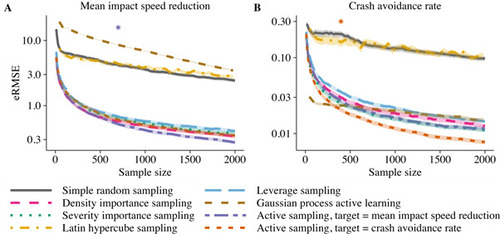
We evaluated the performance of the active sampling method for estimating the mean impact speed reduction or crash avoidance rate of an AEB system compared to baseline driving (without AEB). Active sampling performance was evaluated against simple random sampling, importance sampling, Latin hypercube sampling (Cioppa and Lucas, 2007; Meng et al., 2021), leverage sampling (Ma et al., 2015, 2022), and active learning with Gaussian processes. Two importance sampling schemes were considered: a density sampling scheme with probabilities proportional to the prior observation weights p_i , and a severity sampling scheme that additionally attempts to oversample high-severity instances (i.e., with low deceleration and long glances). Each subsampling method was repeated 500 times up to a total sample size of n = 2, 000 observations. The performance was measured by the root mean squared error of the estimator (eRMSE) compared to ground truth, calculated as in (6). The results are presented graphically as functions of the sample size, i.e., the number of baseline-AEB simulations pairs.

Implementation

The empirical evaluation was implemented using the R language and environment for statistical computing, version 4.2.1 (R Core Team, 2023). Active sampling was implemented with a batch size of n_k = 10 observations per iteration. Random forests (Breiman, 2001) were used for the learning step of the algorithm. We also performed sensitivity analyses for the choice of machine learning algorithm using extreme gradient boosting (Chen and Guestrin, 2016) and k-nearest neighbors. Latin hypercube sampling was implemented similarly to Meng et al. (2021). Statistical leverage scores for the leverage sampling method were calculated using weighted least squares with the two auxiliary variables (off-road glance duration and maximal deceleration during braking) as explanatory variables and the prior scenario probabilities p_i as weights. The Gaussian process active learning method was implemented using a probabilistic uncertainty scheme, with probabilities proportional to the posterior uncertainty (standard deviation) of the predictions. This was chosen based on computational considerations and to promote exploration of the design space. For Gaussian process active learning, estimation was conducted using a model-based estimator by evaluating the predictions over the entire input space. All other methods used observed data rather than predicted values for estimation. Further implementation details are provided in Section B in the Supplement. The R code and data are available in the Supplementary Material and at https://github.com/imbhe/ActiveSampling.

6.2 Results

Confidence interval coverage rates

The empirical coverage rates of large-sample normal confidence intervals under active sampling are presented in Figure 4. There was a clear under-coverage in small samples, as expected. Both the pooled Sen-Yates-Grundy estimator and bootstrap variance estimator produced confidence intervals that approached the nominal 95% confidence level relatively quickly as the sample size increased. Coverage rates were somewhat lower with the martingale variance estimator, and more iterations where needed before the nominal 95% level was reached.

Active sampling performance evaluation

The eRMSE with active sampling compared to five benchmark methods is presented in Figure 5. Simple random sampling and Latin hypercube sampling overall performed worst and had similar performance. Active learning using Gaussian processes had good performance for the crash avoidance (which was relatively constant over the input space, with 80% of all crashes avoided by the AEB), but poor performance for the impact speed reduction (which varied more and was harder to predict). With the other methods, estimation variance in the early iterations was largely driven by the variance of the scenario probability weights in the subsample. In contrast, estimation variance for the model-based (Gaussian process) response surface estimator was attenuated by evaluating predictions over the entire input space. Leverage sampling and the two importance sampling schemes had similar performance, with a slight advantage of severity importance sampling for estimating the crash avoidance rate. Active sampling optimized for a specific characteristic had best performance on the characteristic for which it was optimized. Significant improvements compared to the best performing benchmark method were observed from around 400 samples for estimating the crash avoidance rate and 700 observations for estimating the mean impact speed reduction.

The benefit of active sampling increased with the sample size. At n = 2, 000 observations, a reduction in eRMSE of 20–39% was observed compared to importance sampling. Accordingly, active sampling required up to 46% fewer observations than importance sampling to reach the same level of performance on the characteristic for which it was optimized. Moreover, active sampling performance was on par with that of traditional methods when evaluated on characteristics other than the one it was optimized for. Similar results were observed when using k-nearest neighbors and extreme gradient boosting as auxiliary models for the learning step of the active sampling algorithm (Supplemental Figure S7).

Active sampling was also relatively fast and required about 60 seconds for running 200 iterations (generating n = 2, 000 samples) on a laptop computer equipped with an AMD Ryzen™7 PRO 585OU 1.90 GHz processor. The Gaussian process active learning method required approximately 270 seconds to generate the same number of samples.

7 Discussion

We have presented an active sampling framework for finite population inference with optimal subsamples. Active sampling outperformed standard variance reduction techniques in non-linear settings, and also in linear settings with moderate signal-to-noise ratio. We evaluated the performance of active sampling for safety assessment of advanced driver assistance systems in the context of crash-causation-based scenario generation. Substantial improvements over traditional importance sampling methods were demonstrated, with sample size reductions of up to 50% for the same level of performance in terms of eRMSE. In our application, active sampling was also superior to space-filling, leverage sampling, and Gaussian process active learning methods.

Our work contributes to the ongoing development of subsampling methods in statistics and for computer simulation experiments in particular. In this context, Gaussian processes and space-filling methods have been particularly popular and shown great success for a variety of tasks (Cioppa and Lucas, 2007; Sun et al., 2017; Feng et al., 2020; Batsch et al., 2021; Lim et al., 2021). In our application, however, neither space-filling methods nor Gaussian process active learning performed as well as importance sampling or active sampling. Although we cannot rule out that another implementation of the Gaussian process active learning method could have had better performance, the active sampling framework is less model-dependent and thus is superior for finite population inference. Furthermore, we have proved theoretically that active sampling provides consistent estimators under general conditions. This was also confirmed in our experiments. In our application, we believe that the model-based (Gaussian process) approach to computer experiment emulation is affected by the high complexity of our problem, involving not only one but 44 response surfaces (one per original crash event) that must be learned simultaneously. Yet, this is a fairly small example for scenario generation problems (cf. Ettinger et al., 2021; Duoba and Baby, 2023) and comprises only a fraction of the crashes in the original crash database (Isaksson-Hellman and Norin, 2005). Substantial sample sizes would be needed to accurately model all of the response surfaces. Active sampling, targeting a much simpler problem, requires only a rough sketch of the response surface(s) to identify which regions are most informative for estimating the characteristic of interest.

The choice of batch size influenced the performance of the active sampling algorithm, although less so when the number of iterations were large. In practice, one may need to balance the benefits of a smaller batch size on increased statistical efficiency with the benefits of a larger batch size (involving fewer model updates) on increased computational efficiency. With flexible machine learning methods and proper hyper-parameter tuning, carefully avoiding overfitting, we expect this to hold irrespective of the dimension of the problem, although in higher dimensions larger batch sizes may be favored both for computational efficiency and numerical stability. The choice of prediction model had limited influence on performance, as long as the model was flexible enough to capture the true signals in the data. In computer simulation experiment applications, both computational aspects and anticipated performance should be considered for choosing an appropriate model. It is also possible to utilize several machine learning algorithms in the early iterations of the active sampling algorithm to identify the computationally simplest possible model that does not compromise the accuracy of the estimate. Importantly, active sampling was never worse than simple random sampling, even for a misspecified model. Moreover, using an overly complex model (e.g., a non-linear auxiliary model when the true association is linear) only resulted in a minor loss of efficiency of the active sampling estimator. In contrast, ignoring prediction uncertainty resulted in poor performance, particularly in non-linear settings and for misspecified models.

This paper illustrated the active sampling method in an application to generation of simulation scenarios for the assessment of automated emergency braking. In this application, the computation time for running the active sampling algorithm is orders of magnitudes smaller than the computation time for running the corresponding virtual computer experiment simulations. The computational overhead of the training and optimization steps of the active sampling algorithm is thus negligible. The gain in terms of sample size reductions for a given eRMSE therefore translates to a corresponding reduction in total computation time of equal magnitude. The precision obtained by active sampling at n = 2, 000 observations corresponds to an error margin of about ± 0.5 km/h for the mean impact speed reduction and ±1.0 percentage points for the crash avoidance rate, which may be considered sufficient in a practical setting. This corresponds to savings of about 95% in computation time compared to complete enumeration. Not only can the method be applied more broadly in the traffic safety domain, such as for virtual safety assessment of self-driving vehicles of the future, but it can be applied to a wide range of subsampling applications. Future research on the topic may pursue more efficient methods of partitioning the dataset into areas where the outcomes are more precisely predicted or known (where subsampling is less useful) and those where outcomes are less precisely predicted, as well as demonstrate practical applications further.

8 Conclusion

We have introduced a machine-learning-assisted active sampling framework for finite population inference, with application to a deterministic computer simulation experiment. We proved theoretically that active sampling provides consistent estimators under general conditions. It was also demonstrated empirically to be robust under different choices of machine learning model. Methods for variance and interval estimation have been proposed, and their validity in the active sampling setting was confirmed empirically. Properly accounting for prediction uncertainty was crucial for the performance of the active sampling algorithm. Substantial performance improvements were observed compared to traditional variance reduction techniques and response surface modeling methods. Active sampling is a promising method for efficient sampling and finite population inference in subsampling applications.

Acknowledgment

We would like to thank Volvo Car Corporation for allowing us to use their data and simulation tool, and in particular Malin Svärd and Simon Lundell at Volvo for supporting in the simulation setup. We further want to thank Marina Axelson-Fisk and Johan Jonasson at the Department of Mathematical Sciences, Chalmers University of Technology and University of Gothenburg, for valuable comments on the manuscript.

Funding

This research was supported by the European Commission through the SHAPE-IT project under the European Union’s Horizon 2020 research and innovation programme (under the Marie Skłodowska-Curie grant agreement 860410), and in part also by the Swedish funding agency VINNOVA through the FFI project QUADRIS. Also Chalmers Area of Advance Transport funded part of this research.

Conflict of interest

The authors report there are no competing interests to declare.

SUPPLEMENTARY MATERIAL

Supplemental methods and results: Additional theoretical results and proofs (Section A), details on the implementation of the sampling methods in the application (Section B), and additional experiment results (Section C). (.pdf file)

R code and data: R code and data used for the empirical evaluation in Section 5, application in Section 6, and replication of main results (Figure 3–5). (.zip file). Also available at https://github.com/imbhe/ActiveSampling.

Note

¹ In the non-adaptive setting, the linear estimator is given by $N^{-1}\sum _{i\in \mathcal{S}}{S}_i{w}_i{y}_i$ and the Hájek estimator by ${\widehat{N}}^{-1}\sum _{i\in \mathcal{S}}{S}_i{w}_i{y}_i,\widehat{N}=\sum _{i\in \mathcal{S}}{S}_i{w}_i$.

Figure 1 A: Simulated impact speed reduction with an automatic emergency braking system (AEB) compared to a baseline manual driving scenario (without AEB) in a computer experiment of a rear-end collision generation. In the bottom right corner, no crash was generated in the baseline scenario; such instances are non-informative with regards to safety benefit evaluation. B: Corresponding optimal active sampling scheme. Active sampling oversamples instances in regions where there is a high probability of generating a collision in the baseline scenario (attempting to generate only informative instances) and with a large predicted deviation from the average. These instances will be influential for estimating the safety benefit of the AEB system.

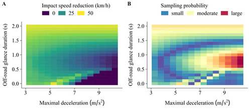
Figure 2 Examples of three synthetic datasets with varying degree of non-linearity. Data were generated according to a Gaussian process, using a Gaussian kernel with bandwidth σ.

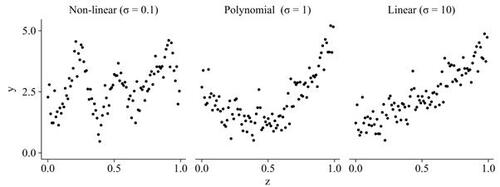
Figure 3 Performance of active sampling using a linear surrogate model (LM) or generalized additive surrogate model (GAM) compared to simple random sampling, ratio estimator, control variates, and importance sampling for estimating a finite population mean in a strictly positive scenario (all $y_i>0$) using a linear estimator ( $h(u)=u/N$) and batch size n_k = 10. Results are shown for 12 different scenarios with varying signal-to-noise ratio (R²) and varying degree of non-linearity (σ) (cf. Figure 2). Shaded regions are 95% confidence intervals for the root mean squared error of the estimator (eRMSE) based on 500 repeated subsampling experiments. Asterisks show the smallest sample sizes for which there were persistent significant improvements (p <.05) with active sampling compared to simple random sampling.

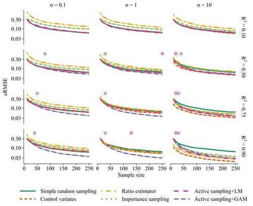
Figure 4 Empirical coverage rates of 95% confidence intervals for the mean impact speed reduction (A) and crash avoidance rate (B) using active sampling. The lines show the coverage rates with three different methods for variance estimation in 500 repeated subsampling experiments. A batch size of n_k = 10 observations per iteration was used.

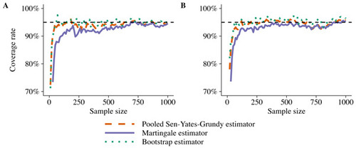
Figure 5 Root mean squared error (eRMSE) for estimating the mean impact speed reduction (A) and crash avoidance rate (B). The lines show the performance using simple random sampling, importance sampling, Latin hypercube sampling, leverage sampling, Gaussian process active learning, and active sampling optimized for the estimation of the mean impact speed reduction and crash avoidance rate. Shaded regions represent 95% confidence intervals for the eRMSE based on 500 repeated subsampling experiments. Asterisks show the smallest sample sizes for which there were persistent significant improvements (p <.05) with active sampling compared to the best performing benchmark method.