Evolutionary hyper-heuristic for solving the strip-packing problem

Abstract

Strip-packing problem (marker making) is an optimization problem, where a set of cutting parts needs to be placed on a marker so that the items do not overlap, and do not exceed the boundaries of a marker. In this research a novel Grid algorithm is introduced, and improvement methods: Grid-BLP and Grid-Shaking. These algorithms were combined with genetic algorithm, and a novel placement order All equal first. An individual representation of a genetic algorithm has been developed that is consisted of placement sequence, rotation of a cutting part, the choice of a placement algorithm, and dynamic grid parameter. Experiments were conducted to determine the best placement algorithm for a dataset, and hyper-heuristic efficiency. The implementation has been developed and experiments were conducted in MATLAB using GEATbx toolbox on five datasets from textile industry: ALBANO, DAGLI, MAO, MARQUES and MAN SHIRT. The marker efficiency in percentage was recorded with best results: 85.17, 81.76, 78.67, 84.67 and 87.19% obtained for the datasets, respectively.

Keywords:

• Strip-packing
• marker making
• genetic algorithm
• grid algorithm
• optimization

1. Introduction

In computer science, a strip-packing problem (marker making, lay-planning) is a combinatorial optimization problem, where a set of items, i.e. cutting parts CP= {cp₁, cp_2, …, cp_n}, $n=\left|CP\right|$, need to be placed on a marker M so that items cp_i and cp_j do not overlap ($c{p}_i\cap c{p}_j=0$) and items do not exceed the boundaries of a marker ($c{p}_i\cap M=c{p}_i$). Cutting parts are defined as irregular polygons, and marker is considered to be a rectangular shaped container, as in (Egeblad, 2008). Since cutting parts are irregularly shaped the problem is often referred to as nesting problem as in (Wäscher, Haußner, & Schumann, 2007).

The strip-packing problem is commonly known as marker/pattern making, pattern layout or lay plan in garment industry as presented in report (Guo, Wong, Leung, & Li, 2011). In garment manufacturing, a set of cutting parts needs to be optimally allocated on a material in order to maximize material utilization and to reduce the amount of waste.

The aim of this research was to develop novel algorithms for solving the strip-packing problem that would achieve competitive results, with possible application in small businesses, to optimize the garment production and influence their productivity. A novel algorithm called Grid is introduced, alongside its two modifications Grid-BLP and Grid-Shaking. The latter two algorithms are compaction algorithms that tighten the placement and improve the Grid solution.

To obtain the solution a genetic algorithm is employed as an optimization tool. The main role of genetic algorithm is to guide the search process and to optimize parameters. The motivation was to set the human interference on the optimization process to the minimum. Therefore, a novel individual representation for the genetic algorithm has been designed. In algorithms in the literature a permutation representation of an individual is mostly used to define the order of placement of cutting parts on a marker. Individual representation used in this research consists of four parts. In the permutation part a placement order of cutting parts is defined. In the rotation part the rotation angle of a cutting part is defined. Also, a parameter that can choose one of three different placement algorithms is added, so that each individual in a population may be placed according to a different method (hyper-heuristic). Finally, a dynamic grid method has been developed that optimizes the density of the grid.

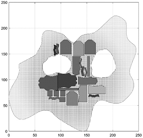
The main benefits of Grid algorithm is its universal application and flexibility. The Grid algorithm is able to place any kind of regular or irregular polygon (cutting part) on any kind of marker, whether it is a rectangular material, irregularly shaped leather (Figure 1), leather with defects or even holes (Figure 2). Therefore, it can be applied on any type of dataset.

Figure 1. Placement of dataset MAO on an irregularly shaped marker.

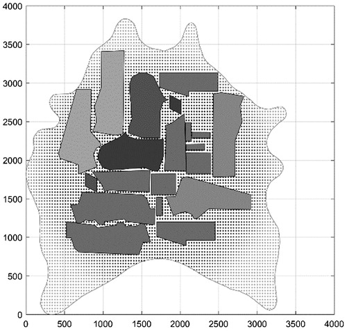
Figure 2. Placement of dataset ALBANO on an irregularly shaped marker with holes.

The benefit of Grid algorithm is that it works with cutting parts directly – it does not need any kind of approximation to lower the complexity. In many papers approximations of cutting parts are created as bounding boxes or simplified polygons with smaller number of vertices to lower the computational complexity.

2. Methodology

In this research three algorithms have been introduced: Grid, Grip-BLP, and Grid-Shaking. The most basic one of three is the Grid algorithm that places the cutting part on the first available grid point that satisfies the conditions. Since some waste (blank) space may still remain between the cutting parts, which may result in lower density marker quality, compaction algorithms: Grid-BLP and Grid-Shaking have been introduced. These algorithms are applied on the solution obtained by Grid algorithm in order to improve it.

2.1. Grid algorithms

A Grid algorithm is a 2 D method used to place cutting parts on a marker. It is based on a Dotted-board model described in (Toledo, Carravilla, Ribeiro, Oliveira, & Gomes, 2013). In the most basic version of Grid algorithm, a set of points is created and equidistantly distributed in x and y direction on the marker (Eq. 1-4). (1) $$d\left(x_i-x_{i-1}\right)-d\left(x_{i+1}-x_i\right)=0$$(1)

(2) $$d\left(y_i-y_{i-1}\right)-d\left(y_{i+1}-y_i\right)=0$$(2) (3) $$x_{i-1}\le x_i\le x_{i+1}$$(3) (4) $$y_{i-1}\le y_i\le y_{i+1}$$(4)

The number of points in grid in both x and y direction is defined as an individual parameter (as defined in Section 2.4.1.) and may vary from individual to individual in genetic algorithm even in the same generation.

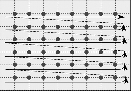
A cutting part is placed on marker so that its reference point (most bottom and left point of its bounding box) coincides with an available grid point. An available grid point is found by following the search direction, i.e. from left to right, and from bottom to the top of marker (Figure 3). Afterwards, a test is performed to determine whether the cutting part fits into the boundaries of a marker and whether it overlaps with the partial layout, i.e. previously placed cutting parts.

Figure 3. Empty grid and search direction.

An example of a placement of the first nine cutting parts from a MAN SHIRT dataset using Grid is presented in Figure 4, where numbers on the cutting parts represent the order in which they were placed on marker). By using the Grid method the waste space between cutting parts can be filled if a cutting part of appropriate size is available in the placement order (Figures 4c–e^{Figure 5}).

Figure 4. An example of cutting part placement on grid points and gap filling.

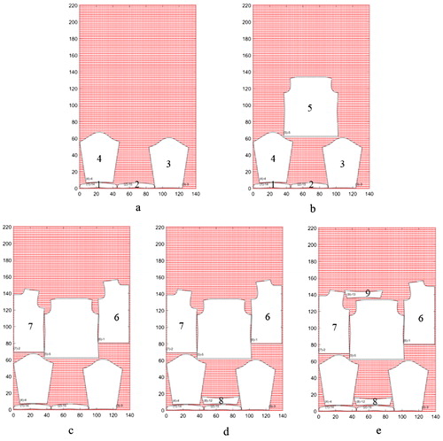
Figure 5. Pseudocode of grid variants.

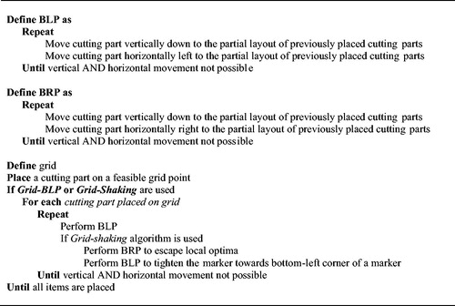
Improvement algorithms Grid-BLP and Grid-Shaking have been developed in this research. These algorithms combine the representation of a marker and the placement used in Grid, with a BLP or Shaking heuristics. These algorithms are inspired by the bottom-left heuristics and are used to obtain placement with higher efficiency.

Bottom-left (BL) is a heuristic placement routine that places polygons on a marker in a series of downwards and leftwards sliding movements. It was first applied on a rectangle placement problem in (Jakobs, 1996). Starting from the top-right corner, polygon is moved vertically downwards until it touches the partial layout, and then horizontally to the left until a polygon is touching the current placement contour from its left and bottom side.

When dealing with placement of irregular items, sliding algorithms based on rectangles (BL_, BLLT, BLD) and sliding algorithms based on polygons (BLP, BLDP, BLF) are examined in (Hopper, 2000).

In the newly developed Grid-BLP algorithm, a sliding algorithm based on polygons called BLP, as it is defined in (Hopper, 2000), is used in this research with Grid. After choosing the position of a cutting part based on Grid, waste space may appear between a cutting part and the partial layout. Therefore, the last placed cutting part is nested using iterative horizontal and vertical moves, i.e. BLP procedure, starting from the current position in a polygonal layout until a stable placement is found. A stable position of a cutting part is a position in which a cutting part cannot be moved more to the left or down without violating overlapping restrictions.

Sometimes a cutting part could have been nested even lover to the left in the partial layout, but that placement has not been obtained because BLP only moves down and left. Cutting part has been caught in the local optima. Therefore, a Grid-Shaking algorithm has been introduced to move cutting part from a local optima. Grid-Shaking applies the BLP and BRP (bottom-right) procedure iteratively. A BRP procedure is performed on the cutting part by performing a sequence of horizontal right and down movements, until a stable position is found. Shaking algorithm uses a procedure to escape local optima that moves the cutting part away from the stable position in which it has been trapped after the BLP has found a stable position.

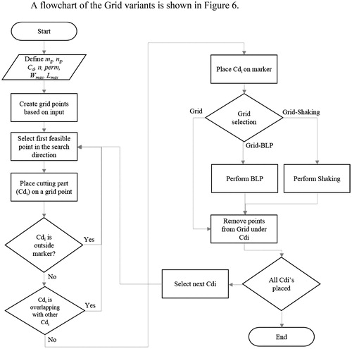
A pseudocode of Grid variants is presented in Figure 5. A flowchart of the Grid variants is shown in Figure 6.

Figure 6. Block diagram of Grid, Grid-BLP and Grid-Shaking algorithm.

2.2. All equal first (AEF) placement order

In Grid algorithm cutting parts are placed on a marker in order determined by the sequence permutation which is obtained with GA. Several equal cutting parts can often be found in a dataset (e.g. front and back cutting part of a shirt). For example, as defined in (EURO Special Interest Group on Cutting and Packing, 2015), dataset ALBANO is consisted of 24 cutting parts, while there are only eight different cutting parts in total, i.e. eight distinct groups of cutting parts – four groups of four, and four groups of two identical replicas of the same cutting part.

Therefore, a placement of groups of equal cutting parts All equal first (AEF) has been developed. The main benefit of AEF is reducing the search space. Without AEF, the search space would have been n!, which corresponds to the number of different permutations in lexicographic order, and n is the number of cutting parts in a dataset. If n_cp(n_cp<n) is the number of groups of different cutting parts in a dataset, the search space is reduced to n_cp!.

In order to implement the AEF placement order, a new individual representation for the genetic algorithm had to be invented that would suit the need of obtaining the results for this research, where each permutation sequence has been assigned an integer value in order to comply with the restrictions of the GEATbx toolbox used in the research, and for the MATLAB’s precision limitations.

The factorial number system used by (Knuth, 1997), which is also known as factoradic in combinatorics, is a mixed radix numeral system used for numbering permutations. If a number less than n! is converted to factorial representation, a sequence of n digits is obtained that can be converted to a permutation of n, either by using them as Lehmer code or as inversion table representation as in (Knuth, 1998). An algorithm for such a mapping is presented in (Knuth, 1997).

A decoding procedure had to be developed to transform the placement sequence of a group of equal elements into placement order of individual elements (Figure 7). An integer part of the individual is transformed to factoradic form, and then into a permutation sequence perm representing groups of cutting parts which are supposed to be placed on a marker based on the lexicographic order from this permutation. Perm is consisted of n_cp elements indicating groups of elements, and is subjected to decoding process to obtain a permutation of n elements. An example of decoding n_cp permutation perm= [5 4 1 6 3 2 8 7] that defines the order of placement groups into seq permutation that defines the order of cutting parts is shown in Figure 8.

Figure 7. Mapping between integers and permutation.

Figure 8. Decoder example for ALBANO dataset for seq = [13 14 15 16 … 21 22].

The integer decoder algorithm also takes into consideration the rotation of cutting parts for 180°. In the implementation a rotation for any arbitrary angle can be taken into consideration.

AEF is used for order sequence in all versions of genetic algorithm in this research.

2.3. Dynamic grid

Dynamic grid is a parameter of a novel individual representation in genetic algorithm. With dynamic grid, the grid size parameters (number of points in x-direction and y-direction; values can be defined separately) are a part of an individual in GA’s population. That way the genetic algorithm directly influences the parameter definition and further improvement across the generations.

The benefit of using dynamic grid is that, within the same generation, various grid densities are investigated alongside the placement order of cutting parts. That way the influence of grid density on the marker density can be determined. In each generation, up to n grid sizes may be tested, where n is the number of individuals in GA, instead of using just one grid size for each generation.

2.4. Genetic algorithm

Genetic algorithm (GA) is a metaheuristic algorithm based on evolutionary computation. As presented in (Golub, 2004), GA mimics nature’s evolution principle that describes the survival of the fittest. GA author, John H. Holland, presented the algorithm in the 1970s motivated by Darwin's theory of evolution. GA uses evolutionary methods to search the solution space in order to find a solution to the optimization problem.

The algorithm starts with initializing a population i.e. a set of individuals called chromosomes. Initial population is usually generated randomly within the solution space to enable searching the entire solution space. Population size depends on the type of problem, but usually the size from a few dozen to a few hundred individuals is used.

The algorithm continues with the selection process where a certain number of individuals from initial populations are selected based on their fitness to enter the reproductive process (recombination and mutation). Fitness of an individual is calculated using a fitness function f(x). Individuals with greater fitness value are considered to pass good properties to their offspring in the recombination process, and improve the quality of the population in the coming generations.

Recombination is a process of producing new individuals (offspring) by inheriting genetic material from individuals in a population (i.e. reproduction process). Individuals are reproducing in order to maintain the good properties of the population. The higher the fitness of an individual, the greater the likelihood of its survival and recombination. In the recombination process one or two offspring are created. The purpose of recombination is to create new individuals, i.e. offspring that will be just as good as or better than their parents.

After crossover some individuals mutate. Mutation is used in GA to escape local optima. Upon completion of the mutation, the new individuals are evaluated and copied into the population. Poor specimens are removed from the population. The process of selection and reproduction is repeated until the termination condition is met.

In the selection process a stochastic universal sampling described in Pohlheim (2003) is used in this research, alongside discrete recombination from Schlierkamp-Voosen and Mühlenbein (1993) and integer mutation.

According to Dasgupta, Papadimitriou, and Vazirani (2006), termination condition may include maximum number of iterations, maximum number of fitness function evaluations, the desired fitness function value, etc.

Genetic algorithm is looking for the best solution in a feasible solution space. Search space is an area of all possible solutions to a problem. One possible solution is represented by one individual in a population. A solution is feasible if it complies with the constraints of the problem. In GA, the search for the best solutions results with creating new solution in a search space.

In this research the GA is hybridized with Grid algorithms to obtain high quality results. Except for the genetic algorithm, evolutionary strategies in Wong and Leung (2009), mixed-integer programming in Fischetti and Luzzi (2009), other methods based on evolutionary computation (e.g. particle swarm optimization in Shalaby (2013)) are also used in the literature.

2.4.1. Novel individual representation

An example of a novel individual representation is depicted in Figure 9.

Figure 9. Individual representation.

Each individual consists of four parts:

1. Permutation

2. Rotation

3. Placement algorithm

4. Grid density

The size of defined individual is n_p+n + 3, where n is the number of cutting parts to be placed on marker, i.e. size of a dataset, and n_p is the number of different groups of cutting parts.

In the permutation section of an individual the order in which cutting parts are placed on a marker is defined. For example, in Figure 9, the fifth cutting part from a dataset will be placed on the marker first, followed by the third cutting part with and so on. Cutting parts are taken based on the order in this section.

The second part of an individual is the rotation part. Each gene can take the integer value n from a set {0, 2}. Rotation angle is n$\times$90°. The cutting parts are rotated or not to comply with the restrictions posed by marker making in textile technology. Each rotation gene is connected to its correspondent order gene. If cp_i is the ith cutting part in a dataset, and n is the number of cutting parts in a dataset, the corresponding rotation gene has index n + i within the chromosome.

The third part of the chromosome is the hyper-heuristic parameter that determines the algorithm which will place the cutting parts on the marker. The value is an integer number from a set {1, 2, 3}.

In order to comply with the GEATbx limitations in individual representation, a permutation part of an individual is represented as integer (Figure 10) which is later decoded to permutation as is described in Section 2.2.

Figure 10. Chromosome representation using radix.

The reason for that was imposed for two reasons. The first is the shortcoming of the GEATbx toolbox, designed by Pohlheim (2007), which is used for genetic algorithm implementation within this research. By Pohlheim (1998), individuals in GEATbx can be represented as: integer numbers, real numbers, permutation and binary tree. Multiple different data types within one individual can not be presented at the same time (e.g. one section of an individual is integer, the other section is permutation). Therefore, factoradic was used to decode integer value into permutation sequence, since a natural mapping between integers when presented in factoradic form and permutations exists. Therefore, the genetic algorithm in GEATbx uses individuals with integers values, while the fitness functions decodes integers into permutation sequence, i.e. a placement order of cutting by using this representation the possibilities of the GEATbx toolbox have been improved.

The last part of the individual holds the information of the number of grid point in the x and y coordinate direction. The values are integer number, and in this research they are in range x= [90, 110] and y = 90, 110].

2.4.2. Hyper-heuristic approach

Just as grid density is a part of an individual in GA, so is the algorithm in which cutting parts need to be placed on marker. Besides the Grid, Grid-BLP and Grid-Shaking algorithm, a hyper-heuristic approach Grid-All is developed, that is able to choose between three different algorithms for parts placement.

By its initial definition by Burke et al. (2013), a hyper-heuristic is a high-level approach that, given a particular problem instance and a number of low-level heuristics, can select and apply an appropriate low-level heuristic at each decision point.

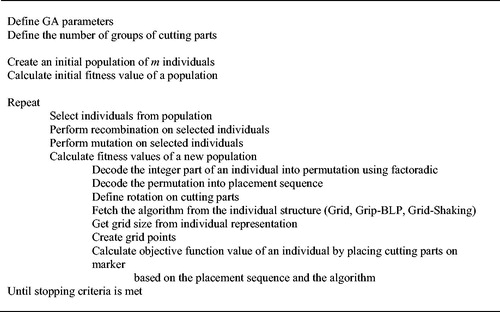
The Grid-All algorithm uses a novel individual representation to change the parameter regarding the placement algorithm choice even within the same population. Each individual in generation can use different algorithm for the placement of cutting parts: Grid, Grid-BLP or Grid-Shaking. The pseudocode for the Grid-All algorithm is shown in Figure 11.

Figure 11. Hyper-heuristic Grid-All algorithm.

2.5. Data sets

In computer science experiments to investigate marker making are conducted on four datasets: ALBANO, DAGLI, MAO and MARQUES that can be obtained from EURO Special Interest Group on Cutting and Packing (2017) in order to benchmark our obtained results with the ones obtained in the literature. These datasets are polygonal approximations of cutting parts in clothing industry for the sake of lower computational complexity, but in remainder of the paper they will be referenced as cutting parts. A dataset MAN SHIRT, which consists of real cutting parts for a man shirt, has been developed. The information about datasets is shown in Table 1.

Table 1. Datasets features.

Dataset	Number of different pieces	Number of cutting parts	Rotations	Shapes	Source
ALBANO	8	24	0, 180	Polygons, non-polygonal pieces with arcs	Scanned from sample layout in paper; approximated by polygons
DAGLI	10	30
MAO	9	20
MARQUES	8	24
MAN SHIRT	10	17			Real cutting part made in Lectra

2.6. Experimental environment and parameters

Applications have been implemented in MATLAB environment following the algorithms in Section 2. For genetic algorithm, a GEATbx (Genetic and Evolutionary Algorithms) toolbox has been used by Pohlheim (2007).

2.6.1. GA parameters

Parameters described in Table 2 are used in the GEATbx toolbox. One population consisted of 25 individuals is used in reproduction process of genetic algorithm in 50 generations. Best individual found upon this termination criterion is considered as the best solution.

Table 2. GEATbx parameters for grid algorithms with and without the dynamic grid.

Parameter		Value
Number of individuals		25
Number of generations		50
Number of experiments iterations per dataset		30
Selection	Name	Stochastic Universal Sampling
	Selective Pressure	1.6
	Generation Gap	0.96
Recombination	Name	Discrete recombination
Mutation	Name	Integer mutation
Termination	Name	Maximum number of generations

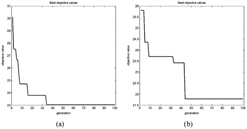
During the preliminary research experiments have been conducted with 100 generations of GA. A significant change in fitness function value has not been obtained after the 50th generation (Figure 12) or the desired change was not significant. Therefore, 50 generations have been chosen, which resulted with faster performance.

Figure 12. Fitness function in experiments with 100 generation of GA.

Stochastic universal sampling has been used for selection, with pressure factor equal to 1.6 and generation gap equal to 0.96. The value of selective pressure determines the fitness assignment and is used by the ranking algorithm, since fitness assignment is always done by ranking. As defined in Pohlheim (2007), generation gap determines the fraction of the population to be reproduced in every generation, i.e. it describes how many individuals will be produced in comparison to the number of individuals in the population. If generation gap equals to 1, than the same amount of offspring as parents is produced and all parents are replaced with offspring. Still the toolbox remembers the best individual found in all generations. If generation gap is less than 1, less offspring than parents is produced so parents with best solutions are able to survive to the next generation (elitism). In this research 24 new offspring will be produced (0.96 × 25 = 24) in each generation and one individual is always kept as best individual (elitism).

Fitness function is calculated using (5): (5) $$f\left(x\right)=1-(\text{area}CP/\text{area}BB),$$(5)

where areaCP is the area of real non approximated cutting parts obtained after the placement algorithm (Grid algorithms), and areaBB is the area of the marker.

3. Results and discussion

Three novel algorithms for marker making were introduced in this research and compared for its efficiency. Grid algorithm is the basic algorithm using which cutting parts are placed on the first feasible point of a grid. Since some waste (blank) space may still remain between the cutting parts, which may result in lower marker efficiency, the compaction algorithms: Grid-BLP and Grid-Shaking have been introduced in order to improve Grid algorithm’s efficiency. It was therefore assumed:

1. By applying the Grid-BLP and Grid-Shaking algorithms, markers with higher efficiency will be obtained compared to the markers developed by applying the Grid algorithm.

2. By applying the Grid-Shaking algorithm the best results for all datasets will be obtained, since a local optima can be avoided.

The efficiency of a hyper-heuristic placement has been calculated to determine which grid algorithm obtains a marker with the best efficiency with genetic algorithm, enabled rotation for 180°, AEF placement, and dynamic grid.

Experiments have been conducted with Grid, Grid-BLP and Grid-Shaking algorithms individually to determine the best placement algorithm. These results are compared with the results of a hyper-heuristic placement Grid-All to determine the percentage of choosing the best placement algorithm by the hyper-heuristic, the efficiency of obtained markers, and to confirm hypothesis:

• 3. By applying the hyper-heuristic Grid-All highest quality markers will be obtained.

• 4. Hyper-heuristic Grid-All will choose the best algorithm in most cases, for a particular data set.

For each dataset and algorithm 30 experiments have been conducted, and several parameters are recorded: the worst (minimum) and the best (maximum) obtained solution, the arithmetic mean of the 30 measurements (the results of placement density in percentage), the range between the minimum and the maximum solution, standard deviation, variance and the standard error.

In Figure 13, a comparison of all mean results for all datasets is shown.

Figure 13. Comparison of average mean results of all algorithms on all test datasets.

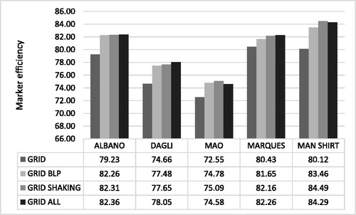
Grid algorithm obtains the worst results for all datasets and the Grid-Shaking obtained the best mean results for all algorithms. Therefore, hypothesis (1) and (2) are valid. It is proven Grid-BLP and Grid-Shaking escape the local optima.

In Table 3, the results of hyper-heuristic Grid-All efficiency are presented, i.e. the percentage of results Grid-Shaking obtained the best result for a dataset. In the remaining cases a Grid-BLP algorithm had obtained better results. Hyper-heuristic has never obtained the best results using Grid algorithm.

Table 3. Hyper-heuristic efficiency.

Dataset	Efficiency (%)
ALBANO	80.00
DAGLI	83.33
MAO	70.00
MARQUES	76.67
MAN SHIRT	90.00

Hyper-heuristic Grid-All did not always choose Grid-Shaking, due to the fact the search space is large since three algorithms can be chosen. In individual algorithm experiments, only a single algorithm has been used. However, the best results out of 30 obtained per algorithm has always been obtained when Grid-Shaking was chosen by the hyper-heuristic. Therefore, the hypothesis (3) is partially valid, and hypothesis (4) is valid.

The overall best results obtained in this research have been noted in Table 4 with a comparison with known results from the literature. Only Hopper (2000) used bottom-left methods in her research. The results of this research outperform all off Hopper’s results and are competitive with other researches as well. None of the authors relied on the AEF order but rather on order obtained by permutation. AEF placement order has been used since humans tend to group elements together, and to place bigger elements on the marker first, the aim was to investigate whether placing the equal cutting parts together will produce denser placements. The results obtained in Efi Optitex (2017) are also presented.

Table 4. Comparison with results in literature.

Author dataset	Hopper (2000)	Egeblad, Nielsen, and Odgaard (2007)	Bennell and Song (2010)	Shalaby (2013)	Optitex	Grid algorithms
ALBANO	84.09	87.88	87.88	83.36	86.37	85.17
DAGLI	77.10	87.05	87.99	83.97	82.20	81.76
MAO	68.65	85.15	84.07	78.4	79.42	78.67
MARQUES	82.73	89.82	88.92	86.47	85.89	84.67
MANSHIRT	–	–	–	–		87.19

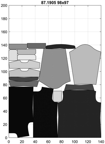
In Figures 14–18, the overall best results for presented.

Figure 14. The overall best result for ALBANO.

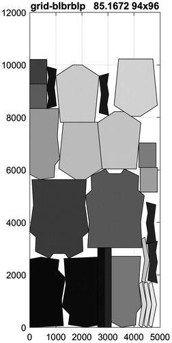
Figure 15. The overall best result for DAGLI.

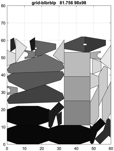
Figure 16. The overall best result for MAO.

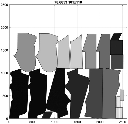
Figure 17. The overall best result for MARQUES.

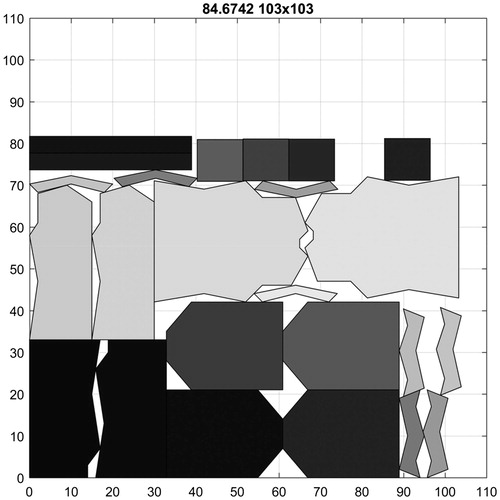
Figure 18. The overall best result for MAN SHIRT.

4. Conclusion

In this article novel algorithms: Grid, Grid-BLP, Grid-Shaking, and a hyper-heuristic approach were introduced. A novel placement order All equal first (AEF) has been introduced using which all equal cutting parts are placed on the marker first, before proceeding to the equal cutting parts of other groups. Algorithms were hybridised with genetic algorithm. An individual representation that consists of: permutation section, rotation section, hyper-heuristic section where a placement algorithm is chosen, and the section where the grid density is defined (dynamic grid). An evolutionary hyper-heuristic Grid-All was introduced that uses a placement defined in the individual structure.

Experiments have been conducted to determine the efficiency of hyper-heuristic placement and to determine which grid algorithm creates a marker with the highest efficiency. It has been shown that by applying the Grid-BLP and Grid-Shaking algorithms markers with higher efficiency than with the Grid algorithm have been obtained, with Grid-Shaking obtaining the best results for all datasets since it can escape local optima.

The best results of a hyper-heuristic version Grid-All has always been obtained by the Grid-Shaking algorithm, but this approach did not always obtain the best results overall as it was assumed, because the flexibility in choosing the placement algorithm increased the search space.

Additional information

Funding

This work has been fully supported by Croatian Science Foundation under the project number 3011 Application of mathematical modeling and intelligent algorithms in clothing construction.

References

- Bennell, J. A., & Song, X. (2010). A beam search implementation for the irregular shape placement problem. Journal of Heuristics, 16(2), 167–188. doi: 10.1007/s10732-008-9095-x
- Burke, E. K., Gendreau, M., Hyde, M., Kendall, G., Ochoa, G., Özcan, E., & Qu, R. (2013). Hyper-heuristics: A survey of the state of the art. Journal of the Operational Research Society, 64(12), 1695–1724. doi: 10.1057/jors.2013.71
- Dasgupta, S., Papadimitriou, C. H., & Vazirani, U. V. (2006). Algorithms. Retrieved from http://www.cse.ucsd.edu/∼dasgupta/mcgrawhill/
- Efi Optitex. (2017). Optitex (Version 12.3) [Computer software]. Retrieved from https://www.optitex.com
- Egeblad, J. (2008). Heuristics for multidimensional placement problems. Københavns Universitet, Faculty of Science, Datalogisk Institut, Department of Computer Science. Retrieved from http://forskningsbasen.deff.dk/Share.external?sp=S659a8b80-ac03-11de-bc73-000ea68e967b&sp=Sku
- Egeblad, J., Nielsen, B. K., & Odgaard, A. (2007). Fast neighborhood search for two- and three-dimensional nesting problems. European Journal of Operational Research, 183(3), 1249–1266. doi: 10.1016/j.ejor.2005.11.063
- EURO Special Interest Group on Cutting and Packing. (2017). albano_2007-05-15, dagli_2007-05-15, mao_2007-04-23, marques_2007-05-15 [Datasets]. Data sets – ESICUP – EURO Special Interest Group on Cutting and Packing. Retrieved from https://www.euro-online.org/websites/esicup/data-sets/#1535972088237-bbcb74e3-b507
- Fischetti, M., & Luzzi, I. (2009). Mixed-integer programming models for nesting problems. Journal of Heuristics, 15(3), 201–226. doi: 10.1007/s10732-008-9088-9
- Golub, M. (2004). Genetski algoritam: Prvi dio. Retrieved from http://www.zemris.fer.hr/∼golub/ga/ga_skripta1.pdf
- Guo, Z., Wong, W., Leung, S., & Li, M. (2011). Applications of artificial intelligence in the apparel industry: A review. Textile Research Journal, 81(18), 1871–1892. doi: 10.1177/0040517511411968
- Hopper, E. (2000). Two-dimensional placement utilising evolutionary algorithms and other meta-heuristic methods (Doctoral Thesis). University of Wales, Cardiff. Retrieved from http://vmk.ugatu.ac.ru/c%26p/article/HOPPER/PhDisser/part1.pdf
- Jakobs, S. (1996). On genetic algorithms for the placement of polygons. European Journal of Operational Research, 88(1), 165–181. doi: 10.1016/0377-2217(94)00166-9
- Knuth, D. E. (1997). The art of computer programming, Volume 2: Seminumerical algorithms (3rd ed.). Boston, MA: Addison-Wesley Longman Publishing Co., Inc.
- Knuth, D. E. (1998). The art of computer programming, Volume 3: Sorting and searching (2nd ed.). Redwood City, CA: Addison Wesley Longman Publishing Co., Inc.
- Pohlheim, H. (1998). Genetic and evolutionary algorithm toolbox for use with MATLAB. Ilmenau, Germany: Dept. Comput. Sci., Univ. Ilmenau. Retrieved from http://www.geatbx.com/download/GEATbx_Tutorial_v33c.pdf
- Pohlheim, H. (2003). Evolutionary algorithms. Heidelberg: Springer. Retrieved from http://www.geatbx.com/download/GEATbx_Intro_Algorithmen_v37.pdf
- Pohlheim, H. (2007). GEATbx: Genetic and evolutionary algorithms toolbox in Matlab. Retrieved from http://www.geatbx.com/
- Schlierkamp-Voosen, D., & Mühlenbein, H. (1993). Predictive models for the breeder genetic algorithm. Evolutionary Computation, 1(1), 25–49. doi: 10.1162/evco.1993.1.1.25
- Shalaby, M. A., & Kashkoush, M. (2013). A particle swarm optimization algorithm for a 2-D irregular strip placement problem. American Journal of Operations Research, 03(02), 268–278. doi: 10.4236/ajor.2013.32024
- Toledo, F. M. B., Carravilla, M. A., Ribeiro, C., Oliveira, J. F., & Gomes, A. M. (2013). The Dotted–Board model: A new MIP model for nesting irregular shapes. International Journal of Production Economics, 145(2), 478–487. doi: 10.1016/j.ijpe.2013.04.009
- Wäscher, G., Haußner, H., & Schumann, H. (2007). An improved typology of cutting and placement problems. European Journal of Operational Research, 183(3), 1109–1130. doi: 10.1016/j.ejor.2005.12.047
- Wong, W. K., & Leung, S. Y. S. (2009). A hybrid planning process for improving fabric utilization. Textile Research Journal, 79(18), 1680–1695. doi: 10.1177/0040517509102225