Fundamentals of vehicle–track coupled dynamics

Abstract

This paper presents a framework to investigate the dynamics of overall vehicle–track systems with emphasis on theoretical modelling, numerical simulation and experimental validation. A three-dimensional vehicle–track coupled dynamics model is developed in which a typical railway passenger vehicle is modelled as a 35-degree-of-freedom multi-body system. A traditional ballasted track is modelled as two parallel continuous beams supported by a discrete-elastic foundation of three layers with sleepers and ballasts included. The non-ballasted slab track is modelled as two parallel continuous beams supported by a series of elastic rectangle plates on a viscoelastic foundation. The vehicle subsystem and the track subsystem are coupled through a wheel–rail spatial coupling model that considers rail vibrations in vertical, lateral and torsional directions. Random track irregularities expressed by track spectra are considered as system excitations by means of a time–frequency transformation technique. A fast explicit integration method is applied to solve the large nonlinear equations of motion of the system in the time domain. A computer program named TTISIM is developed to predict the vertical and lateral dynamic responses of the vehicle–track coupled system. The theoretical model is validated by full-scale field experiments, including the speed-up test on the Beijing–Qinhuangdao line and the high-speed running test on the Qinhuangdao–Shenyang line. Differences in the dynamic responses analysed by the vehicle–track coupled dynamics and by the classical vehicle dynamics are ascertained in the case of vehicles passing through curved tracks.

Keywords:

• train–track interaction
• vehicle dynamics
• vehicle–track coupled dynamics
• curving performance
• experimental validation

1. Introduction

The classical theory of railway vehicle dynamics 1 2 usually focuses on the railway vehicle itself as the analysis object without consideration of the dynamic behaviour of the track system that supports the vehicle, i.e. the track structure is assumed to be a rigid base. In fact, the railway track is a typical elastic structure with damping. Vibrations of the vehicle can be transmitted to the track via the wheel–rail contact and excite vibrations of the elastic track structure, which can in reverse influence the vibrations of the vehicle not only in the vertical direction but in the lateral direction as well. Therefore, the vibrations of a vehicle and a track are essentially coupled with each other.

With the increase in train speed and vehicle axle load, effects of the dynamic interaction between the vehicle and the track obviously intensify. Dynamic effects of the vehicle on the track structure increase accordingly, especially in the case of increasing the train speed on existing railway track structures such as in Chinese Railways (CR) 3. Furthermore, a great interest of modern railway designers as well as maintenance engineers is motivated by the desire to improve ride comfort, to prevent vehicle hunting, to reduce deformations of the track, to minimise damage and wear of both vehicle and track components and, most important of all, to ensure running safety. All above aspects relate to the dynamic behaviour of the entire vehicle–track system. Well understanding the dynamic characteristics of the entire system provides the possibility to optimise the design parameters of both the vehicle and the track components that would minimise the dynamic interactions between the vehicle and the track. Therefore, it is necessary to systematically investigate the dynamics of a vehicle and a track from the entire vehicle–track system. This is the basic idea of the vehicle–track coupled dynamics, which was already adopted by the author in the early 1990s 4–6.

In fact, it seems to be a trend to consider the vehicle and the track as an integral system in recent studies on track dynamics and on wheel–rail dynamic interactions 7–19. The rapid development of computation technique makes it easy to analyse a large complicate vehicle–track coupled system. However, most of the research work deals with vertical dynamic problems. Very few can be found on the lateral system dynamics 8 11 16 19. It is important to analyse the lateral dynamic behaviour of a vehicle running on a viscoelastic track structure instead of a rigid track. Our field experiment results 20 showed that the lateral displacement of the top of the rail could reach 4–5 mm for the wooden sleeper track and 2–3 mm for the concrete sleeper track when a freight train is passing through a 287 m radius curve. The maximum values of the gauge enlargement corresponding to these two cases were measured to be about 9 mm and about 3 mm, respectively. So large lateral motions of the rails will definitely cause great changes in the wheel–rail contact geometry and will thereby eventually influence the lateral and vertical wheel–rail dynamic forces. It is not clear how big the difference is between the lateral dynamic indices predicted by the models with and without consideration of track vibration, for example the difference between the lateral wheel–rail forces on a curved track with a rigid track model and with an elastic track model. It is also not very clear which parameters of the track system have a significant influence on the lateral dynamic performance of the vehicle as well as on the lateral vehicle–track interaction.

This paper intends to systematically introduce the framework of the vehicle–track coupled dynamics with emphasis on new advances made by the authors in recent years. A three-dimensional model of a typical passenger coach on a ballasted track will be described in detail. A dynamic model of a non-ballasted track is also developed in consideration of the wide application of this type of track on high-speed railways. Random track irregularities varying with the rail longitudinal direction are simulated based on the track spectra and used as excitation input to the vehicle–track coupled system. The models will be validated using field measurement data obtained from the speed-up test on the Beijing–Qinhuangdao line and from the high-speed test on the Qinhuangdao–Shenyang line. Special attention will be paid to the differences of the curving performances analysed with the vehicle–track coupled dynamics and with the classical vehicle dynamics without consideration of elastic track structures.

2. Theoretical model

A vehicle–track coupled model is the theoretical foundation for analysing the vehicle–track interaction. During the last decade, a series of vehicle–track system models have been established for various research purposes. A vertical and lateral coupling model for a freight car with three-piece bogies and a ballasted track was published in an early paper by the author in 1996 11. A similar model for the vertical and lateral dynamics of the wagon–track system was presented by Sun et al. in 2003 16. This paper will present a three-dimensional coupled model for typical passenger coaches and tracks including the non-ballasted slab track.

2.1. Three-dimensional vehicle–track coupled model

Figures 1–3 illustrate the various components of the three-dimensional vehicle–track model in which subsystems describing the vehicle and the track are spatially coupled by the wheel–rail interface.

Figure 1. Three-dimensional vehicle–track coupled model (elevation).

Figure 2. Three-dimensional vehicle–track coupled model (planform).

Figure 3. Three-dimensional vehicle–track coupled model (end view).

In the vehicle submodel, the car body is supported on two double-axle bogies at each end. The bogie frames are linked with the wheelsets through the primary suspensions and linked with the car body through the secondary suspensions. Three-dimensional spring–damper elements are used to represent the primary and the secondary suspensions. Yaw dampers and anti-roll springs are considered in the secondary suspensions. Furthermore, the lateral clearances between the car body and the stop-blocks on the bogie frames are also considered in the secondary suspensions. The vehicle is assumed to move along the track with a constant travelling speed. Each component of the vehicle has five degrees of freedom (DOFs): the vertical displacement Z, the lateral displacement Y, the roll angle Φ, the yaw angle ψ and the pitch angle β with respect to its centre of mass (the pitch for a wheelset corresponds to the variation of rotation around its mean rotational speed). All angles are assumed to be small, which simplifies the kinematics and the equations of motion. As a result, the total DOFs of the passenger vehicle submodel are 35.

The track submodel shown in Figures 1 and 3 represents the typical ballasted track structure, consisting of rails, rail pads, sleepers, the ballast and the subgrade. Both the left and the right rails are treated as continuous Bernoulli–Euler beams which are discretely supported at rail–sleeper junctions by three layers of springs and dampers, representing the elasticity and damping of the rail pad, the ballast and the subgrade, respectively. The model allows the input of track parameters varying along the rail’s longitudinal direction, such as sleeper spacing or track supporting stiffness. Three kinds of vibrations of the rails are considered: vertical Z _r , lateral Y _r and torsional Φ _r . The sleeper is assumed to be a rigid body with three DOFs of the vertical displacement Z _s , the lateral displacement Y _s and the roll angle displacement Φ _s . Lateral springs and dampers are considered to represent the lateral dynamic properties in the fastener system. Similarly, the lateral springs and dampers are used to represent the elasticity and damping property between the sleeper and the ballast in the lateral direction.

For modelling the ballast, a five-parameter model of ballast under each rail-supporting point is adopted 6 21, which is based upon the hypothesis that load transmission from a sleeper to the ballast approximately coincides with cone distribution 22. Only the vertical motion Z _b of the ballast mass is taken into account. In order to account for the continuity and the coupling effects of the interlocking ballast granules, a couple of shear stiffness (K _w ) and shear damping (C _w ) is introduced between adjacent ballast masses in the ballast model. The ballast model was recently modified 21 to be able to cover the practical situation in which an overlapping of adjacent ballast masses may occur, see Figure 4. In this case, the vibrating mass of ballast under a rail-support point could be defined as the shadowed region as shown in Figure 4, where h ₀ is the height of the overlapping regions, h _b is the depth of ballast, l _s is the sleeper spacing, l _b is the width of sleeper underside and α is the ballast stress distribution angle.

Figure 4. Modified model of the ballast.

If the analysed track structure is a non-ballasted track such as the slab track, the above track dynamic model should be changed correspondingly. Figures 5 and 6 show the established three-dimensional slab track model in which the track slabs are described as elastic rectangle plates supported on viscoelastic foundation. In Figure 6, K _sv and C _sv are the vertical stiffness and damping of the CA layer, and K _sh and C _sh are the lateral stiffness and damping of the CA layer, respectively. Because the lateral bending stiffness of the slab is very large, it is sufficient to consider the rigid mode of the slab vibration in the lateral direction.

Figure 5. Three-dimensional slab track model (elevation).

Figure 6. Three-dimensional slab track model (end view).

2.2. Equations of motion

2.2.1. Equations of motion of vehicle subsystem

By using the system of coordinates moving along the track with vehicle speed, the equations of motion of the vehicle subsystem can be easily derived according to D’Alembert’s principle, which can be described in the form of second-order differential equations in the time domain: (1) where X _V , V _V and A _V are the vectors of displacements, velocities and accelerations of the vehicle subsystem, respectively; M _V is the mass matrix of the vehicle; C _V (V _V ) and K _V (X _V ) are the damping and the stiffness matrices which can depend on the current state of the vehicle subsystem to describe nonlinearities within the suspension; X _T and V _T are the vectors of displacements and velocities of the track subsystem; F _V(X _V ,V _V,X _T,V _T ) is the system load vector representing the nonlinear wheel–rail contact forces determined by the wheel–rail coupling model, which depend on the motions X _V and V _V of the vehicle and X _T and V _T of the track; and F _EXT describes external forces including gravitational forces and forces resulting from the centripetal acceleration when the vehicle is running through a curve 23.

Figure 7. Nonlinear characteristic of a yaw damper.

There are several nonlinear factors existing in the suspension systems of passenger cars, e.g. the nonlinear yaw dampers and the clearances between the car body and the stop-block on the bogie frames. Generally, the yaw damper has a saturation nonlinearity, as shown in Figure 7. The damping force of a yaw damper can be described by (2) where is the saturation force of the damper; v _xct is the relative velocity between two ends of the damper connecting the car body and the bogie frame in the longitudinal direction; and v ₀ is the unloading velocity of the damper.

Figure 8. Lateral clearance between the car body and the stop-block on the bogie frame.

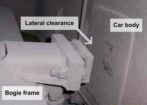
Figure 8 shows a picture of a stop-block on the bogie frame used in the secondary suspension. It can be clearly seen there is a lateral clearance between the car body and the stop-block on the bogie frame. If the lateral clearance disappears, the car body will contact the stop-block and a large contact stiffness will contribute to the secondary stiffness, as shown in Figure 9. Therefore, the lateral force of a secondary suspension can be given by (3) where δ _sc is the lateral clearance between the car body and the stop-block; K _sy is the lateral stiffness of the secondary spring; K _sc is the contact stiffness in the lateral direction if the car body is in contact with the stop-block; Y _cb is the relative displacement between two ends of the secondary spring connecting the car body and the bogie frame in the lateral direction.

Figure 9. Nonlinear characteristic of lateral stiffness in the secondary suspension.

2.2.2. Equations of motion of track subsystem

The equations of motion of the track subsystem are more complex than those of the vehicle subsystem due to the spatial continuity of rails and slabs. The equations of motion of rails are given in form of the fourth-order partial differential equations:

Vertical vibration: (4)

Lateral vibration: (5)

Torsional vibration: (6) In Equations ( 4)–( 6), Z _r(x, t), Y _r(x, t) and Φ_r(x, t) are the vertical, lateral and torsional displacements of the rail, respectively; m _r is the rail mass per unit length; ρ is the rail density; EI _y and EI _z are the rail bending stiffness to the Y-axle and to the Z-axle, respectively; I ₀ is the torsional inertia of the rail; GK is the rail torsional stiffness; F _{sv i} (t) and F _{sl i} (t) are the vertical and lateral dynamic forces at the ith rail-supporting point; P _j (t) and Q _j (t) are the jth wheel–rail vertical and lateral forces; M _si (t) and M _{w j} (t) are the moments acting on the rails due to the forces F _{sv i} (t) and F _sli (t) and due to the forces P _j (t) and Q _j (t), respectively; and δ(x) is the Dirac delta function.

Figure 10. Forces acting on the cross-section of the rail.

The moments M _{s i} (t) and M _{w j} (t) can be determined based on the forces acting on the rail cross-section, as shown in Figure 10: (7) where a is the vertical distance between the rail torsional centre and the lateral force from the fastening system; b is half of the distance between two vertical forces from the fastening system; h _r is the vertical distance from the rail torsional centre to the lateral wheel–rail force; and e is the lateral distance from the rail torsional centre to the vertical wheel–rail force.

By describing the slab as a plate supported by a viscoelastic foundation, the vertical vibrations of each slab are given by: (8) For the lateral motions, the slab is considered as a rigid body. Thus, the lateral vibrations are described by: (9) where (10) in Equations ( 8)–( 10), w(x, y, t) and y _s are the vertical and lateral displacements of the slab; C _s is the damping of the slab; D _s is the vertical bending stiffness of the slab; ρ _s is the slab density; L _s , W _s and h _s are the length, width and thickness of the slab, respectively; F _{CAv j} (t) and F _CAlj (t) are the vertical and lateral dynamic forces at the jth supporting point under the slab; E _s and ν _s are Young’s elastic modulus and Poisson’s ratio of the slab; N _p and N _b are the total number of rail fasteners on one slab and the total number of discrete supporting points under one slab used in the calculation.

In order to solve the track subsystem equations with the time-stepping integration method, the fourth-order partial differential equations of rails and slabs must be transformed into a series of second-order ordinary differential equations in terms of the generalised coordinates, which could be done by means of Ritz’s method 6 11. The transformation results for the rail equations could be found in 11. It should be pointed out that sufficient numbers of rail modes are necessary to describe the vibrations of the track system. Numerical trial results show that 0.5L/l _s is enough to be chosen as the rail mode number to study the present vehicle–track coupled dynamics, where L is the effective length of the rail used in the calculation.

For the slab equation ( 8), the solution can be assumed as (11) where X _m (x) and Y _n (y) are the mode functions of the slab with x and y coordinates respectively; T _{m n} (t) is the generalised coordinate in terms of time t; m and n are the mode numbers of X _m (x) and Y _n (y), respectively; and N _x and N _y are the total mode numbers of the slab mode functions X _m (x) and Y _n (y) selected for the calculation.

For the rectangle plate supported on the viscoelastic foundation with free boundaries, the mode functions X _m (x) and Y _n (y) are given by: (12---) where α _m and ϵ _n are the frequency coefficients corresponding to X _m (x) and Y _n (y), and β _m and ξ _n are the mode coefficients corresponding to X _m (x) and Y _n (y), respectively. (13---) (14---) Substituting Equation ( 11) into Equation ( 8) yields (15) Multiplying Equation ( 15) by X _k (x)Y _h (y) and then applying integral in the slab area yields the second-order ordinary differential equations of the slab vertical vibration in terms of the generalised coordinate T _{m n} (t) as follows: (16) where m=1,2,…,N _x , n=1,2,…, N _y . Due to the orthogonality of the mode functions, the integrals vanish for k ≠ m and h ≠ n. (17)

Therefore, the final equations of the track subsystem, either for the ballasted track structure including the equations of the sleepers and ballast blocks which are modelled as individual rigid masses or for the non-ballasted track structure could be expressed in terms of the standard matrix form as (18) where M _T is the mass matrix of the track structure; C _T and K _T are the damping and the stiffness matrices of the track subsystem; A _V is the vector of accelerations of the system; and F _T(X _V ,V _V,X _T ,V _T ) is the load vector of the track subsystem representing the nonlinear wheel–rail forces obtained by the wheel–rail coupling model.

2.3. Wheel–rail coupling model

The wheel–rail coupling model is the essential element that couples the vehicle subsystem with the track subsystem at the wheel–rail interfaces.

Unlike the early wheel–rail contact model used in the classical vehicle dynamics, in which the rails are assumed to be fixed without any movement, the dynamic wheel–rail coupling model for the analysis of the three-dimensional vehicle–track coupled dynamics should consider three kinds of rail motions in vertical, lateral and torsional directions, as shown in Figure 11. In the model, C _Lc and C _Rc are the left and the right wheel–rail contact points and δ _L and δ _R are the left and the right wheel–rail contact angles, respectively. The nonlinear Hertzian elastic contact theory is used to calculate the wheel–rail normal contact forces according to the elastic compression deformation of wheels and rails at contact points in the normal directions, which depends on the displacements of wheels and rails. The tangential wheel–rail creep forces are calculated first by the use of Kalker’s linear creep theory and then modified by the Shen–Hedrick–Elkins nonlinear model 24. Details of the new wheel–rail coupling model could be found in a recent paper by Chen and Zhai 25.

Figure 11. Wheel–rail coupling model.

The new spatial wheel–rail coupling model eliminates the assumption that the wheel and the rail are in contact all the time as used in the classical vehicle dynamics. Thus the current model is capable of dealing with the situation that the wheel loses its contact with the rail existing in practical railway operations, which may provide a new path to simulate the dynamic process of derailment.

3. System excitation

As we know, the vehicle–track coupled vibrations are mainly excited by irregularities on the surfaces of wheels and rails. Generally, there are two types of geometric irregularities existing at the wheel–rail system. One type is specific irregularities such as the wheel flat, the out-of-round wheel, the dipped rail-joint and the rail corrugation, etc., which has been widely discussed in the literature. The other type is random irregularities such as the roughness on the surfaces of wheels and rails, which mainly influence the wheel–rail rolling noise, and the random deviation of the track geometry. Random track irregularities exist in railway lines everywhere and influence the dynamic performance of vehicles moving on tracks. This paper will focus on the excitation by the random irregularity of the track.

The random track irregularity is usually expressed by a one-sided power spectrum density (PSD) function, namely track spectrum. The PSD function of the track spectrum measured on CR mainlines is expressed as a unified formula (19) where the unit of S(f) is mm²/(1/m); f=1/λ is the spatial frequency in cycle/m (λ is the wavelength, λ>1 m); A to G are the specific parameters which are different for vertical and lateral rail irregularities. Table 1 gives the values of these parameters for the CR speed-raised railway lines such as the Beijing–Shanghai line and the Beijing–Guangzhou line. Figure 12 compares the CR track spectrum with the AAR track spectra. It can be seen from Figure 12a that the rail vertical profile irregularities of the CR track spectrum are usually located between those of the AAR 5th class spectrum and 6th class spectrum. Figure 12b shows that the rail alignment irregularities of the CR track spectrum are larger than those of the AAR 5th class spectrum if 1 m<λ<7 m, smaller than those of the AAR 5th class spectrum if λ>15 m, and approximately the same at the wavelength range from 7 to 15 m.

Table 1. Values of parameters of the CR mainline track spectrum.

Parameter	A	B	C	D	E	F	G
Left rail vertical	1.1029	−1.4709	0.5941	0.8480	3.8016	−0.2500	0.0112
Right rail vertical	0.8581	−1.4607	0.5848	0.0407	2.8428	−0.1989	0.0094
Left rail alignment	0.2244	−1.5746	0.6683	−2.1466	1.7665	−0.1506	0.0052
Right rail alignment	0.3743	−1.5894	0.7265	0.4353	0.9101	−0.0270	0.0031
Cross-level	0.1214	−2.1603	2.0214	4.5089	2.2227	−0.0396	0.0073

Figure 12. Comparison of the Chinese track spectrum with AAR track spectra: (a) rail vertical profile irregularities; (b) rail alignment irregularities.

The wavelength λ in the above track spectra is >1 m. In order to excite high-frequency wheel–rail interactions, however, the irregularities with wavelength shorter than 1 m are needed. A measurement result of this type of rail vertical irregularity on the Chinese Shijiazhuang–Taiyuan line is given here 26 (20) where the range of the wavelength is 0.01  m.

In order to input the track spectrum into the vehicle–track system, the PSD function should be transformed into vertical and lateral changes of the rail geometry varying with the track’s longitudinal distance (or in time domain) by means of a time–frequency transformation technique 27. Figure 13 displays samples of the vertical and lateral irregularities of the left and right rails representing the CR mainline condition, which are transformed from Equation ( 19) with parameters listed in Table 1, superposed with vertical short wavelength irregularities on rails in the form of Equation ( 20).

Figure 13. Samples of the vertical and lateral rail irregularities obtained from the CR track spectra: (a) vertical irregularity of the left rail; (b) lateral irregularity of the left rail; (c) vertical irregularity of the right rail; (d) lateral irregularity of the right rail.

4. Numerical solution

Time-stepping integration provides the best way for a numerical solution of the equations of motion of the vehicle–track system including nonlinearities. In order to enhance the computational speed for such a large-scale dynamic system, a simple fast explicit integration method previously developed by Zhai 28 is employed. The scheme of this integration method to calculate the displacement X and the velocity V of a system is expressed as follows: (21) where Δt is the time step; the subscripts n+1, n and n−1 denote the integration time at (n+1)Δt, nΔt and (n−1)Δt, respectively; and ψ and ϕ are free parameters that control the stability and numerical dissipation of the algorithm. Usually a value of 0.5 could be assigned to ψ and ϕ to achieve good compatibility between numerical stability and accuracy.

With the help of this explicit integration method, the solution of the nonlinear vehicle–track coupled dynamics could be easily simplified without solution of any algebraic equation group. For each time step, the integration method is, respectively, applied to the vehicle subsystem and the track subsystem to explicitly calculate the responses of displacements and velocities. The nonlinear wheel–rail contact forces can then be determined based on the calculated displacements and velocities of wheels and rails. With these known results, the accelerations of the vehicle and the track subsystems are finally calculated from the equations of motion of each subsystem. Therefore, the main solution procedure for the vehicle–track coupled dynamics consists of the following six steps:

a.	calculate the displacement X V,n+1 and the velocity V V,n+1 of the vehicle subsystem at the time (n+1)Δt by using Equation ( 21) based on the states of the system at time nΔt and time (n−1)Δt;
b.	calculate the displacement X T,n+1 and the velocity V T,n+1 of the track subsystem at time (n+1)Δt using Equation ( 21) based on the states of the system at time nΔt and time (n−1)Δt;
c.	estimate the wheel–rail normal contact forces and creep forces with the wheel–rail coupling model based on the calculated displacements and velocities of wheels and rails from steps (a) and (b);
d.	calculate the load vectors F V,n+1,F EXT,n+1 and F T,n+1 at time (n+1)Δt from the wheel–rail contact forces and from the external forces due to the curvature, superelevation, etc. for the current position of each body of the vehicle;
e.	compute the acceleration A V,n+1 of the vehicle subsystem from Equation ( 1) at time (n+1)Δt: (22)
f.	compute the acceleration A T,n+1 of the track subsystem from Equation ( 18) at time (n+1)Δt: (23)

Because the mass matrices M _V of the vehicle subsystem and M _T of the track subsystems are diagonal matrices, no algebraic equations have to be solved to obtain the inverse mass matrices and required in Equations ( 22) and ( 23). Thus the computational efficiency is greatly enhanced.

Numerical trial results show that the critical time step of the integration method is Δt _cr =1.5×10⁻⁴ s when used for the solution of the present vehicle–track dynamic system, as shown in Figure 14. In order to get a high calculation accuracy, however, the actually adopted effective time step is suggested to be Δt _e =1.0×10⁻⁴ s.

Figure 14. Stability of the integration method for vehicle–track coupled dynamics: variation of the calculated wheel–rail forces P ₁ and P ₂ with the time step Δt.

5. Computer simulation

Computer simulation is a key technique to obtain the detailed responses of such a large dynamic system. Two computer simulation programs were developed using the above fast integration method to analyse the vehicle–track coupled dynamics. One is named VICT, which was developed in the early 1990s and is used for analysing the vertical dynamic interactions between vehicles and tracks. The basic features and applications of the VICT program could be found in previously published articles; see, for example, 6.

Another program, named TTISIM (Train-Track Interaction SIMulation), was developed by the authors in recent years at Southwest Jiaotong University. It is based on the three-dimensional vehicle–track coupled model involving the new wheel–rail coupling model. The flow chart of the complete simulation process is illustrated in Figure 15.

Figure 15. Flow chart of the TTISIM simulation system.

Unlike the VICT, which is mainly used to analyse vertical dynamic effects of vehicles on tracks, TTISIM can be used to investigate the dynamic behaviour of vehicles running on flexible track structures, including the lateral stability, ride comfort, curving performance, etc. The major difference between TTISIM and other popularly used vehicle system dynamics software might be that the track structure components are modelled in detail in TTISIM. Actual profiles of wheels and rails measured, for example, by the MiniProf device, from existing railways can be directly input to TTISIM as initial data. TTISIM can produce complete responses of the vehicle–track system including the vertical and lateral wheel–rail forces, rail–sleeper forces, vertical and lateral accelerations of car body, bogies and wheelsets, vertical and lateral displacements and accelerations of rails, sleepers and ballasts, etc.

6. Field experimental validation

The three-dimensional vehicle–track coupled models and the simulation program TTISIM have been validated by a lot of field measurements conducted with a variety of vehicles and track conditions representing those of Chinese main trains and mainline tracks. Full-scale field tests include the speed-up test on the Beijing–Qinhuangdao line, the high-speed running test on the Qinhuangdao–Shenyang line and the wheel–rail dynamic interaction experiment on curved tracks of the Chengdu–Chongqing line, etc. In this paper, the main results from the first two tests will be reported and compared with the calculated results obtained from the three-dimensional vehicle–track coupled model.

The speed-up test on the Beijing–Qinhuangdao line was carried out by China Academy of Railway Sciences and Beijing Railway Bureau in December 2000. The tested vehicle is a double-deck passenger coach with two double-axle bogies. The track structure on the tested section is a typical ballasted track used in CR with 60 kg/m rails and general concrete sleepers. The main parameters of the tested vehicle and the track used in the simulation are listed in Tables 2 and 3, respectively.

Table 2. Main parameters of railway vehicles used in the simulation.

Notation	Parameter	Double-deck passenger coach	‘Chinese Star’ power car
M c	Car body mass (kg)	29,600	59,364.2
M t	Bogie mass (kg)	1700	5630.8
M w	Wheelset mass (kg)	1900	1843.5
I cx	Mass moment of inertia of car body about X axis (kg m^2)	5.802×10^4	1.305×10^5
I cy	Mass moment of inertia of car body about Y axis (kg m^2)	2.139×10^6	1.723×10^6
I cz	Mass moment of inertia of car body about Z axis (kg m^2)	2.139×10^6	1.796×10^6
I tx	Mass moment of inertia of bogie about X axis (kg m^2)	1600	2202
I ty	Mass moment of inertia of bogie about Y axis (kg m^2)	1700	9487
I tz	Mass moment of inertia of bogie about Z axis (kg m^2)	1700	11,233
I wx	Mass moment of inertia of wheelset about X axis (kg m^2)	1067	1263
I wy	Mass moment of inertia of wheelset about Y axis (kg m^2)	140	219
I wz	Mass moment of inertia of wheelset about Z axis (kg m^2)	1067	1285
K px	Stiffness coefficient of primary suspension along X axis (MN/m)	24	30.8
K py	Stiffness coefficient of primary suspension along Y axis (MN/m)	5.1	4.878
K pz	Stiffness coefficient of primary suspension along Z axis (MN/m)	0.873	2.399 6
K sx	Stiffness coefficient of secondary suspension along X axis (MN/m)	1.2	0.315 6
K sy	Stiffness coefficient of secondary suspension along Y axis (MN/m)	0.3	0.315 6
K sz	Stiffness coefficient of secondary suspension along Z axis (MN/m)	0.41	0.885 8
C pz	Damping coefficient of primary suspension along Z axis (kN s/m)	30	30
C sy	Damping coefficient of secondary suspension along Y axis (kN s/m)	25	50
C sz	Damping coefficient of secondary suspension along Z axis (kN s/m)	108.7	45
l c	Semi-longitudinal distance between bogies (m)	9.0	5.73
l t	Semi-longitudinal distance between wheelsets in bogie (m)	1.2	1.5
R 0	Wheel radius (m)	0.4575	0.525

Table 3. Main parameters of the ballasted track used in the simulation.

Notation	Parameter	Value (per rail seat)
E	Elastic modulus of rail (N/m^2)	2.059×10^11
ρ	Density of rail (kg/m^3)	7.86×10^3
I 0	Torsional inertia of rail (m^4)	3.741×10^−5
I y	Rail second moment of area about Y axis (m^4)	3.217×10^−5
I z	Rail second moment of area about Z axis (m^4)	5.24×10^−6
GK	Rail torsional stiffness (N m/rad)	1.9587×10^5
m r	Rail mass per unit length (kg/m)	60.64
M s	Sleeper mass (half) (kg)	125.5
K pv	Fastener stiffness in vertical direction (N/m)	6.5×10^7
K ph	Fastener stiffness in lateral direction (N/m)	2.0×10^7
C pv	Fastener damping in vertical direction (N s/m)	7.5×10^4
C ph	Fastener damping in lateral direction (N s/m)	5.0×10^4
l s	Sleeper spacing (m)	0.545
l e	Effective support length of half sleeper (m)	0.95
l b	Sleeper width (m)	0.273
ρb	Ballast density (kg/m^3)	1.8×10^3
E b	Elastic modulus of ballast (Pa)	1.1×10^8
C b	Ballast damping (N s/m)	5.88×10^4
K w	Ballast shear stiffness (N/m)	7.84×10^7
C w	Ballast shear damping (N s/m)	8.0×10^4
α	Ballast stress distribution angle (°)	35
h b	Ballast thickness (m)	0.45
E f	Subgrade K 30 modulus (Pa/m)	9.0×10^7
C f	Subgrade damping (N s/m)	3.115×10^4

In the high-speed running test on the Qinhuangdao–Shenyang line, dynamic responses of a vehicle running on a slab track was measured in 2002. The tested vehicle is a high-speed power car, named ‘Chinese Star’, whose parameters are also given in Table 2. The tested track is a non-ballasted slab track on a curve with a radius of 4000 m and with a superelevation of 115 mm. The length, width and thickness of the slab are 4.93, 2.4 and 0.19 m, respectively. The slab mass per unit length is 1115.62 kg/m. The elastic modulus of the CA layer under the slab is 300 MPa.

6.1. Comparison of dynamic wheel–rail forces

In the speed-up test on the Beijing–Qinhuangdao line, the instrumented wheelsets were installed in the tested vehicle to measure the wheel–rail forces, which provided a possibility for the comparison of time histories of the vertical and lateral wheel–rail forces during vehicle movement.

Figures 16a and 17a give the measured lateral and vertical wheel–rail forces, respectively, when the tested vehicle is running with a velocity of 160 km/h through a curve section with a radius of 1200 m and with a superelevation of 100 mm. The lengths of the circular curve and the transition curve are 142.25 and 100 m, respectively. Figures 16b and 17b show the calculated time responses of the lateral and vertical wheel–rail forces (data given with the same time interval as the measured one). It can be seen from these figures that the time responses of both the lateral and vertical wheel–rail forces predicted by the current vehicle–track coupled model are in reasonable agreement with the field measured responses.

Figure 16. Comparison of measured and calculated lateral wheel–rail forces on a curved track.

Figure 17. Comparison of measured and calculated vertical wheel–rail forces on a curved track.

6.2. Comparison of dynamic responses of vehicle system

For the comparison of vehicle dynamic responses, ride comfort indices are chosen. In consideration of the CR standards, Sperling index is adopted here to evaluate the ride comfort of vehicles, which could be calculated with Sperling’s method based on the car body accelerations and weighted by frequencies 29.

Figures 18 and 19 compare the measured and the calculated lateral and vertical Sperling indices of the car body of the ‘Chinese Star’ power car running on the tested slab track section in the Qinhuangdao–Shenyang line. The measured track irregularities on this high-speed test section are used here as the system excitation. There are good correlations between the calculated results and the measurement data in the tested speed range, as shown in Figures 18 and 19.

Figure 18. Comparison of measured and calculated lateral Sperling indices of the car body.

Figure 19. Comparison of measured and calculated vertical Sperling indices of the car body.

6.3. Comparison of dynamic responses of track system

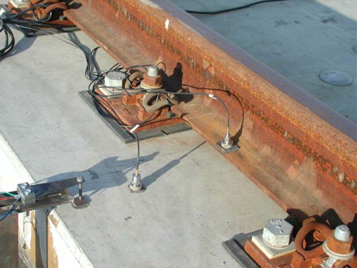
In the high-speed running test on the Qinhuangdao–Shenyang line, the vibrations of the slab track structure were measured by the authors. Figure 20 shows a picture of the position of the accelerometers for measuring the vertical accelerations of the rail and the slab in the experiment.

Figure 20. Accelerometers on the rail and on the slab.

The measured results of peak values of the vertical accelerations of the rail and the slab are given in Figures 21 and 22, respectively, in which the effective frequency band is 0–1500 Hz for the measurement of track accelerations. The calculated results obtained with the current model are also given in these figures, which are close to the measured data. It is shown from Figure 22 that the vertical acceleration of the slab increases tardily with the addition of the train speed in the tested speed range.

Figure 21. Comparison of measured and calculated vertical rail accelerations of the slab track.

Figure 22. Comparison of measured and calculated vertical slab accelerations of the slab track.

7. Case study

In order to ascertain the difference between the computational results obtained with the vehicle–track coupled dynamics model and those obtained with a classical vehicle dynamics model, vehicle curving performances on an elastic track and a rigid track are analysed, respectively. Both results are compared for two cases: general vehicle curving on a very small-radius curve with low speed (case I) and high-speed vehicle curving on a very large-radius curve with high speed (case II).

7.1. Case I: curving on very small-radius curve with low speed

In this case, a very small-radius curve is chosen so that severe lateral dynamic interaction may occur. The radius of the curve is 287 m. The superelevation of the outer rail is 125 mm. The track consists of rails with a mass of 60 kg/m, concrete sleepers and ordinary macadam ballast, which belongs to the Chinese typical ballasted track structure. The vehicle chosen is the Chinese general passenger car, which is the same as that used in the speed-up test on the Beijing–Qinhuangdao line (Section 6). The parameters of the vehicle and the track used here are the same as those given in Tables 2 and 3, respectively. The Chinese mainline track spectra, superposed with the rail short wavelength irregularities in form of Equation ( 20), are used in the calculation. The curving speed of the vehicle is 65 km/h.

Figure 23a and b shows the calculated lateral wheel–rail forces of vehicle curving on an elastic track model (using the vehicle–track coupled dynamics) and on a rigid track model (using the classical vehicle dynamics), respectively. It can be seen that the lateral wheel–rail forces calculated with the vehicle–track coupled dynamics are generally smaller than those obtained with the classical vehicle dynamics. The deviation of both the maximum values is 16.3%. A comparison of the calculated vertical wheel–rail forces for vehicle curving on the elastic track model and on the rigid track model is shown in Figure 24. It can also be seen that modelling the track as an elastic structure leads to smaller dynamic wheel–rail vertical forces than assuming the track to be a rigid base. The maximum deviation of both results is 9.7%.

Figure 23. Calculated lateral wheel–rail forces for vehicle curving on (a) the elastic track model and (b) the rigid track model.

Figure 24. Calculated vertical wheel–rail forces for vehicle curving on (a) the elastic track model and (b) the rigid track model.

In Figures 25 and 26, the PSDs of the lateral and vertical wheel–rail forces obtained with the two models are compared. Figure 25 shows a significant difference for the lateral wheel–rail forces in the frequency range above 20 Hz, whereas little difference can be found at lower frequencies. For the vertical wheel–rail forces, a significant difference is observed for the frequencies >40 Hz, as shown in Figure 26. It could be concluded from this calculation that the high-frequency vibrations of the track lead to differences in the spectral amplitudes. The viscoelastic track structure may absorb some energy relating to the high-frequency vibrations. Of course, the wheelset deformability also has some influence on the high-frequency wheel–rail forces, especially on the vertical force, which needs further research.

Figure 25. Comparison of power spectrum densities of lateral wheel–rail forces obtained from vehicle–track coupled dynamics (elastic track model) and from classical vehicle dynamics (rigid track model).

Figure 26. Comparison of power spectrum densities of vertical wheel–rail forces obtained from vehicle–track coupled dynamics (elastic track model) and from classical vehicle dynamics (rigid track model).

The main reason for the changes in the wheel–rail forces when using the elastic track model is the effect of the rail vibrations actually existing in the curving process. Figures 27–29 depict the main results reflecting the rail lateral dynamic behaviour when the vehicle passes through the curve. It can be seen from Figure 27 that the outer rail is shoved outwards by the lateral wheel–rail forces in the process of curving and the maximum lateral displacement of the rail reaches 1.9 mm. The outer rail rolls over with a maximum rolling angle of 0.38°, as shown in Figure 28. The combination of lateral displacements and rolling of the outer and the inner rails results in a dynamic enlargement of the gauge (Figure 29). The maximum dynamic enlargement of this gauge in the case is 2.1 mm.

Figure 27. Time history of rail lateral displacement during curving.

Figure 28. Time history of rail rolling angle during curving.

Figure 29. Dynamic gauge enlargement during curving.

Compared with the case of fixed rigid rails assumed in the classical theory of vehicle dynamics, where the rail lateral displacement and the rail rolling angle are all equal to zero, the elastic track modelling shows remarkable rail lateral motions during the vehicle curving. This rail lateral motion causes obvious change in positions of the wheel–rail contact points and definitely results in the change of the lateral and vertical wheel–rail dynamic forces.

7.2. Case II: curving on very large-radius curve with high speed

The ‘Chinese Star’ high-speed power car is chosen as an example in this calculation, whose parameters are given in Table 2. The curve has a radius of 6000 m and a maximum superelevation of 70 mm. The length of the transition curve is 180 m. The curving speed of the vehicle is 250 km/h.

Table 4 summarises the main results representing the curving performances calculated with the classical vehicle dynamics model assuming a rigid track and with the vehicle–track coupled dynamics model using an elastic track model. The relative deviations between both results are also given for each dynamic index in Table 4. It is clear from Table 4 that the elastic track model produces much smaller values of dynamic indices than the rigid track model does. The reduction ratios are different for different indices. For example, the reduction ratios of the lateral wheel–rail dynamic force, the vertical wheel–rail dynamic force and the derailment coefficient are 13.02%, 22.06% and 19.44%, respectively.

Table 4. Comparison of high-speed curving performance indices calculated with the classical vehicle dynamics and the vehicle–track coupled dynamics.

Dynamic index	Classical vehicle dynamics	Vehicle–track coupled dynamics	Relative deviation (%)
Wheel–rail lateral force (kN)	28.03	24.38	13.02
Wheel–rail vertical force (kN)	180.79	140.89	22.06
Wheelset lateral force (kN)	18.18	15.77	13.26
Derailment coefficient	0.36	0.29	19.44
Reduction ratio of wheel-load	0.46	0.31	32.61
Dynamic gauge enlargement (mm)	0	0.51	–

8. Conclusions

A framework has been systematically presented in this paper for investigating the overall dynamics of the vehicle–track system. A three-dimensional vehicle–track coupled model has been established in which the vehicle subsystem and the track subsystem are coupled through a spatial wheel–rail coupling model that considers the rail vibrations in vertical, lateral and torsional directions. Random track irregularities varying with the rail’s longitudinal direction have been simulated based on track spectra to excite vibrations of the vehicle–track system. Rail irregularities with short wavelengths are also considered in order to be able to excite the high-frequency wheel–rail interactions. The dynamic responses are solved numerically with a fast integration method in the time domain. The vehicle–track coupled model has been validated by full-scale field experiments, showing good correlation between theoretical and experimental results.

Significant differences between the curving performances obtained from the vehicle–track coupled dynamics and from the classical vehicle dynamics have been found for the cases of a general vehicle curving on a very small-radius curve and a high-speed vehicle curving on a large-radius curve. The deviation is usually located within the range of 10–20%. The vehicle–track coupled dynamics gives smaller values of the curving performance indices than the classical vehicle dynamics modelling does.

It is found that vehicle curving can cause obvious lateral vibrations of rails and can make the rails roll over under the action of lateral wheel–rail forces, resulting in dynamic enlargement of the gauge. The rail’s lateral motion can lead to changes in the position of the wheel–rail contact points, which influences the wheel–rail forces and thereby eventually the curving performance of the vehicle. Therefore, it is necessary to consider the vibration of the track structure when evaluating the curving performance.

The vehicle–track coupled dynamics, including the validated models and the simulation software reported in this paper, provides a method to investigate the dynamic behaviour of the entire vehicle–track system, including the wheel–rail interfaces, and also provides an efficient way to systematically optimise the design parameters of both the vehicle and the track components. A lot of future investigation is possible, for example on dynamic interactions between vehicles and non-ballasted track structures, on the effect of track lateral properties on vehicle lateral running behaviours and on the influence of curve characteristics on ride comfort of high-speed vehicles, etc.

Acknowledgements

This research was supported by National Natural Science Foundation of China (NSFC) under grants 50838006, 50823004 and 50521503 and by National Basic Research Program of China (973 Program) under grant 2007CB714706. The authors would like to thank the reviewers of this paper for their valuable suggestions.

References

- Wickens, A. H. , 2003. Fundamentals of Rail Vehicle Dynamics: Guidance and Stability . Lisse, The Netherlands: Swets & Zeitlinger Publishers; 2003.
- Garg, V. K. , and Dukkipati, R. V. , 1984. Dynamics of Railway Vehicle Systems . Canada: Academic Press; 1984.
- Zhai, W. M. , Cai, C. B. , Wang, Q. C. , Lu, Z. W. , and Wu, X. S. , 2001. Dynamic effects of vehicles on tracks in the case of raising train speed , J. Rail Rapid Transit 215 (2) (2001), pp. 125–135.
- Zhai, W. M. , 1991. Vertical coupling dynamics of vehicle and track as an integral system . Chengdu, China: Southwest Jiaotong University; 1991, Ph.D Thesis, [in Chinese].
- Zhai, W. M. , Wang, K. W. , Fu, M. H. , and Yan, J. M. , Minimizing dynamic interactions between track and heavy haul freight cars . Presented at Proceedings of the 5th International Heavy Haul Railway Conference. Beijing, June, 1993.
- Zhai, W. M. , and Sun, X. , 1994. A detailed model for investigating vertical interaction between railway vehicle and track , Veh. Syst. Dyn. 23 (Suppl.) (1994), pp. 603–615.
- Knothe, K. , and Grassie, S. L. , 1993. Modeling of railway track and vehicle/track interaction at high frequencies , Veh. Syst. Dyn. 22 (3/4) (1993), pp. 209–262.
- Diana, G. , Cheli, F. , Bruni, S. , and Collina, A. , 1994. Interaction between railroad superstructure and railway vehicles , Veh. Syst. Dyn. 23 (Suppl.) (1994), pp. 75–86.
- Nielsen, J. C.O. , and Igeland, A. , 1995. Vertical dynamic interaction between train and track – influence of wheel and track imperfections , J. Sound Vibr. 187 (5) (1995), pp. 825–839.
- Ripke, B. , and Knothe, K. , 1995. Simulation of high frequency vehicle‐track interactions , Veh. Syst. Dyn. 24 (Suppl.) (1995), pp. 72–85.
- Zhai, W. M. , Cai, C. B. , and Guo, S. Z. , 1996. Coupling model of vertical and lateral vehicle/track interactions , Veh. Syst. Dyn. 26 (1) (1996), pp. 61–79.
- Frohling, R. D. , 1998. Low frequency dynamic vehicle–track interaction: Modelling and simulation , Veh. Syst. Dyn. 28 (Suppl.) (1998), pp. 30–46.
- Oscarsson, J. , and Dahlberg, T. , 1998. Dynamic train/track/ballast interaction – Computer models and full‐scale experiments , Veh. Syst. Dyn. 28 (Suppl.) (1998), pp. 73–84.
- Popp, K. , Kruse, H. , and Kaiser, I. , 1999. Vehicle‐track dynamics in the mid‐frequency range , Veh. Syst. Dyn. 31 (5–6) (1999), pp. 423–464.
- Sun, Y. Q. , and Dhanasekar, M. , 2002. A dynamic model for the vertical interaction of the rail track and wagon system , Int. J. Solids Struct. 39 (2002), pp. 1337–1359.
- Sun, Y. Q. , Dhanasekar, M. , and Roach, D. , 2003. A three‐dimensional model for the lateral and vertical dynamics of wagon‐track systems , J. Rail Rapid Transit 217 (2003), pp. 31–45.
- Lei, X. Y. , and Mao, L. J. , 2004. Dynamic response analyses of vehicle and track coupled system on track transition of conventional high speed railway , J. Sound Vibr. 271 (3–5) (2004), pp. 1133–1146.
- Lundqvist, A. , and Dahlberg, T. , 2004. Dynamic train/track interaction including model for track settlement evolvement , Veh. Syst. Dyn. 41 (Suppl.) (2004), pp. 667–676.
- Xu, Y. L. , and Ding, Q. S. , 2006. Interaction of railway vehicles with track in cross‐winds , J. Fluids Struct. 22 (3) (2006), pp. 295–314.
- Zhai, W. M. , and Wang, K. Y. , 2006. Lateral interactions of trains and tracks on small‐radius curves: simulation and experiment , Veh. Syst. Dyn. 44 (Suppl.) (2006), pp. 520–530.
- Zhai, W. M. , Wang, K. Y. , and Lin, J. H. , 2004. Modelling and experiment of railway ballast vibrations , J. Sound Vibr. 270 (4–5) (2004), pp. 673–683.
- Ahlbeck, D. R. , Meacham, H. C. , and Prause, R. H. , 1978. "The development of analytical models for railroad track dynamics". In: Kerr, A. D. , ed. Railroad Track Mechanics & Technology . London: Pergamon Press; 1978.
- Zhai, W. M. , 2007. Vehicle–Track Coupled Dynamics . Beijing: Science Press; 2007, [In Chinese].
- Shen, Z. Y. , Hedrick, J. K. , and Elkins, J. A. , A comparison of alternative creep force models for rail vehicle dynamic analysis . Presented at Proceedings of 8th IAVSD Symposium. June, 1983.
- Chen, G. , and Zhai, W. M. , 2004. A new wheel/rail spatially dynamic coupling model and its verification , Veh. Syst. Dyn. 41 (4) (2004), pp. 301–322.
- Wang, L. , 1988. Random vibration theory of rail track structure and its application in the study of rail track vibration isolation . Beijing: China Academy of Railway Sciences; 1988, Ph.D thesis, [in Chinese].
- Chen, G. , and Zhai, W. M. , 1999. Numerical simulation of the stochastic process of railway track irregularities , J. Southwest Jiaotong Univ. 34 (2) (1999), pp. 138–142, [in Chinese].
- Zhai, W. M. , 1996. Two simple fast integration methods for large-scale dynamic problems in engineering , Int. J. Numer. Methods Eng. 39 (24) (1996), pp. 4199–4214.
- Office for Research and Experiments, 1977. Method for Assessing Riding Quality of Vehicle . Utrecht, The Netherlands. 1977, Report C116/RP8.