Influencing driver chosen cornering speed by means of modified steering feel

Abstract

This paper presents an investigation about influencing the driver's behaviour intuitively by means of modified steering feel. For a rollover indication through haptic feedback a model was developed and tested that returned a warning to the driver about too high vehicle speed. This was realised by modifying the experienced steering wheel torque as a function of the lateral acceleration. The hypothesis for this work was that drivers of heavy vehicles will perform with more margin of safety to the rollover threshold if the steering feel is altered by means of decreased or additionally increased steering wheel torque at high lateral acceleration. Therefore, the model was implemented in a test truck with active steering with torque overlay and used for a track test. Thirty-three drivers took part in the investigation that showed, depending on the parameter setting, a significant decrease of lateral acceleration while cornering.

Keywords:

• steering feel
• steering feel modification
• heavy truck
• driving tests
• driver behaviour
• rollover

1. Introduction

The senses do not deceive, the assessment deceives. (Goethe)

Rollover is a common accident among heavy commercial vehicles that are characterised by a high situated centre of gravity (CoG) in proportion to the track width.[1–3] The most common cause is high lateral acceleration as a result of excessive speed while cornering.[4] One critical road section is the exit lanes of highways. They are often designed as clothoids where the cornering radius decreases continuously. When the speed is not appropriately adjusted, this situation can cause the lateral acceleration to increase in spite of the fact that the vehicle speed decreases. One way to decrease the rollover risk is to develop driver assistance. This work is based on the idea that the driver's assessment can be deceived by a controlled change of the steering feel to warn the driver intuitively. The hypothesis of this investigation is that the drivers’ behaviour can be influenced by means of modified steering feel (MSF). Drivers of heavy vehicles are therefore expected to perform with a greater margin of safety to the rollover threshold if the steering wheel torque is decreased or additionally increased at high lateral acceleration.

Previous work by Katzourakis et al.[5,6] showed that they were able to support the drivers of passenger cars by means of active steering and make them perform better at the driving limit. By means of torque overlay, the steering stiffness was reduced at high lateral acceleration, amplifying the effect of the tyres’ lateral force saturation. In simulator as well as test track experiments, they showed that drivers performed fewer steering corrections and deviated less from their desired trajectory compared with the reference.

Roll control has been investigated by, among others, the following researchers:

Lin et al.[7] showed by simulation that the rollover threshold of a single-unit lorry could be improved by 66% by means of a limited bandwidth hydraulic actuator in series with an anti-roll bar.

Cho et al.[8] designed a unified chassis control that optimises the distribution of yaw moment generation between active front steering and differential braking by means of the electronic stability program (ESC) to optimise vehicle stability and manoeuvrability. However, the investigation was performed on passenger cars that rarely experience the problem of rollover accidents. This becomes even more clear since Cho et al. did not consider lateral acceleration but only vehicle roll, which could be improved by means of continuous damping control (CDC). In their simulations they showed that the vehicle was not necessarily braked as only ESC would achieve. The CDC will, of course, also improve rollover stability; however, it will not prevent rollover in an application with high CoG like a heavy truck.

Gáspár et al.[9] developed a yaw-roll-model controller that combined both path tracking and rollover prevention by means of active steering and active braking based on the linear parameter variation method. They conclude that ‘the controller minimises the tracking error and when the normalised load transfer has reached its critical value, the brake control is also activated in order to prevent the rollover’.

Winkler et al.[10] presented in 1999 a ‘RAS’ (see Figure 1). The system estimated the current rollover threshold and visualised it on a display in combination with the current lateral acceleration. The system was tested with different loads (including an off-centre loaded trailer) and was calibrated on a tilt table. However, the system was not tested in an Human-Machine-Interface (HMI) study, but the inventors aimed more for driver training over time than for an instantaneous warning system.

Figure 1. Roll Stability Advisor (RAS) presented by Winkler et al.[10] showing current lateral acceleration and rollover threshold.

Cheng and Cebon [11] began at the rear-end of the truck–trailer combination and improved the roll stability of an articulated heavy vehicle by means of active semi-trailer steering. A controller optimised the trade-off of path-tracking deviation of the semi-trailer rear-end and the lateral acceleration at its CoG. By simulation they could show a significant improvement of the semi-trailer's roll stability during transient manoeuvres (20% less lateral load transfer).

Futterer et al.[12] investigated rollover mitigation for light commercial vehicles by means of active braking as well as active steering. They concluded that vehicles with high CoG need more intervention by active braking to fulfil the task of avoiding rollover. Only vehicles with lower situated CoG allow a predominant intervention by active steering associated with more agility and preventing deceleration.

The results of Futterer et al.,[12] Gáspár et al.[9] and indirectly of Winkler et al.[10] show the physical limits of rollover prevention. Following a given bend with a certain radius with a certain vehicle speed, will result in a certain lateral acceleration which will act on the CoG. As long as the CoG height and the track width cannot be changed, the only way to decrease the rollover risk is by decreasing cornering speed.

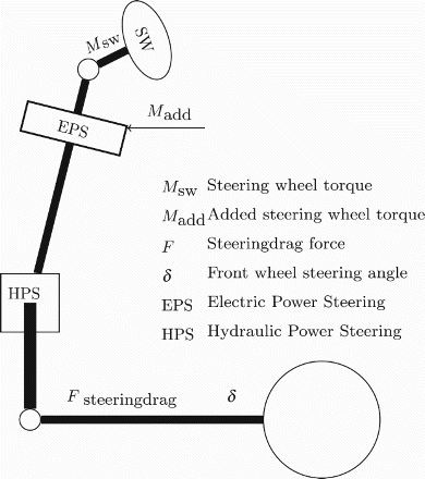
Braking represents the main intervention of ESC systems and as well as the aim of the present study – the reduction of vehicle speed while cornering to prevent rollover. ESC systems usually support the driver by decreasing the vehicle speed as much as necessary by braking and thereby decreasing the risk of rollover. However, ESC is a kind of last chance system. The goal of designing vehicles is to support the driver by making it unnecessary to throw the lifeline. In that way, the better vehicle is the one that makes the driver choose the correct vehicle speed – possibly near the limit but on the right side. Active steering, here meaning the superposition of steering wheel torque (see Figure 2), enables a modification of the steering feel of the vehicle which can be utilised to warn the driver intuitively. Therefore, in a track test the cornering behaviour of 33 drivers was investigated with respect to the lateral acceleration.

Figure 2. Schematic illustration of the active steering system with superposition of torque in a heavy truck for manipulation of steering feel.

The structure of the paper is as follows. In Section 2, a rollover strategy is presented including its safety strategy and the software-in-the-loop development environment. In Section 3, the experiment with test drivers on a closed test track and the procedure is explained. Section 4 focusses on the evaluation of the experiment including a description of the statistical methods used and the results. Section 5 gives a discussion of the results, limitations of the experiment and concluding remarks.

1.1 Problem definition

The research question in this investigation is: How should the steering feel be changed to give the driver an intuitive warning in order to decrease the vehicle speed while cornering to reduce the rollover risk? Other questions in focus are: What will be experienced as intuitive? And how must a system operate to enable the driver to perform better, meaning with more safety margin to the rollover limit?

This paper presents an MSF-functionality that changes the steering feel in case of impending rollover. It will not be able to avoid a rollover accident but it is designed as an intuitive rollover warning to the driver.

2. Rollover indication

2.1 Strategies

In the model for the MSF, there are two main strategies for rollover indication that differ in one parameter:

• Setting 1: The ice-patch strategy. A steering wheel torque is added to the driver's steering input. This decreases the necessary steering torque input for the driver. The steering feel resembles the situation when suddenly driving on low-friction road surface.

• Setting 2: The lane-keeping strategy. A steering wheel torque is subtracted from the driver's steering input. This makes the necessary steering torque input larger for the driver. In other words, the steering feel is similar to the intervention of several lane-keeping assistant systems that operate with superposition of steering torque.

These two strategies are based on different assumptions:

Setting 1 is based on the assumption that the driver expects an increasing resisting torque on the steering wheel when increasing the steering wheel angle at a certain vehicle speed. For many drivers, experiencing a decreasing torque indicates a disturbance at the front wheels, e.g. ice or oil on the road, and will alarm the driver. This means that the feedback-path steering wheel torque is manipulated in a way which indicates slippery road conditions.

Setting 2 is based on the principle that is used in several lane-keeping assistance systems in passenger cars. When leaving the lane, the steering system will steer back to the centre of the lane. Here, the increased steering wheel torque is felt by many of the drivers as an indicator for high lateral acceleration which normally co-occurs with a higher steering wheel torque. Therefore, the feedback-path steering wheel torque is manipulated in a way which indicates higher lateral acceleration than really occurs.

The general conception of manipulation of steering feel for rollover prevention in a heavy truck is illustrated in Figure 3. The added steering wheel torque is expressed as a function of lateral acceleration. The two strategies described above are expressed by the sign of the derivative of the intervention. The intervention could occur already at lower or at higher lateral acceleration (not shown in the figure) and could have different degrees of inclination.

Figure 3. General conception of the presented MSF characteristics for rollover indication in a heavy truck expressed as added steering wheel torque as a function of lateral acceleration.

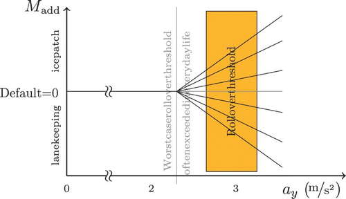
There are several reasons for an early intervention at a low lateral acceleration limit: first, the real rollover threshold varies a great deal between different commercial vehicles depending on several parameters. In any case, a rollover indication should cover all of them. The worst case rollover threshold of heavy vehicles is exceeded often which is an important difference from passenger cars. Another reason for an early intervention is unconscious recognition. Buld and Krüger [13] showed that car drivers use haptic information that is lower than the just noticeable difference (JND).¹ This means that a driver possibly does not consciously recognise the intervention but still receives the information and changes his behaviour. However, the JND is individual and has a wide scatter over a larger population.

2.2 Calculation of added steering torque

The intention and calculation of the added (or subtracted) steering wheel torque can be explained as follows. The driver should feel – consciously or unconsciously – some kind of feedback on the rollover threshold when close to it while cornering. Rollover risk depends first of all on lateral acceleration. This means that an intervention should only occur from a certain level of lateral acceleration. The intervention should increase slowly, not abruptly, to enable smooth driving and subconscious influence. The JND for steering wheel torque spreads a lot for different drivers.[14] Therefore a step-input would be detected by only a few of the drivers or too heavy for others. In addition, the steering input of most of the drivers is smooth. In the same smooth way the rollover risk increases, so an intuitive warning should occur similar smooth. A pre-test showed that a higher increase was only experienced as a heavier intervention, a non-linear intervention like a quadratic or an S-function could not be distinguished from the linear one. As a guideline for the level at which the intervention begins, the ESC intervention limit can be used. However, the steering intervention should begin at a significantly lower limit than ESC, on the one hand because of the different JNDs of different drivers, on the other hand since the driver should be able to adapt the vehicle speed before ESC intervention. In this investigation was chosen after a pre-test. The range under this start value is a dead zone.

In summary there are four inputs and parameters:

• (1) Sign (characteristic option, depending on general strategy) of added torque

• (2) Lateral acceleration

• (3) Slope (correction factor adapting the linear function to the desired output level)

• (4) Dead zone limit (intervention start)

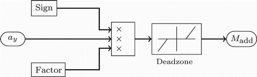
The dead zone around the area where no intervention is desired shifts the linear function to the critical area where the intervention is necessary. Figure 4 shows the base model made in Matlab Simulink.

Figure 4. Matlab Simulink model of MSF functionality for rollover indication.

2.3 Safety

The driver must always be able to control the vehicle in order to make the active steering concept safe. The safety concept is realised here by means of the limitation of the added steering wheel torque () which is easy for every driver to override. This safety concept is implemented in several steps at different positions in the system. Using the hydraulic power system as safe state makes it easier to implement a safety strategy than with other systems.

2.4 Virtual test environment

The MSF function was embedded in a test environment that provided the function with the necessary input values (see Figure 5). In this model, a vehicle and the active steering actuator were emulated and the intervention of the manipulated steering feel function was incorporated. In this pre-study the driver reaction was not taken into consideration.

Figure 5. Active steering functionality in a software-in-the-loop environment.

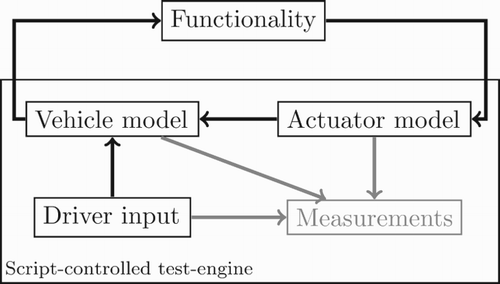
The vehicle model was described here by a bicycle model with tyres modelled according to Magic Formula [15] and rollsteer based on CoG height and a coefficient. The active steering actuator was modelled according to its dynamic properties. The input values were generated (e.g. sine or step steer) or taken from real vehicle measurements.

3. Experiment

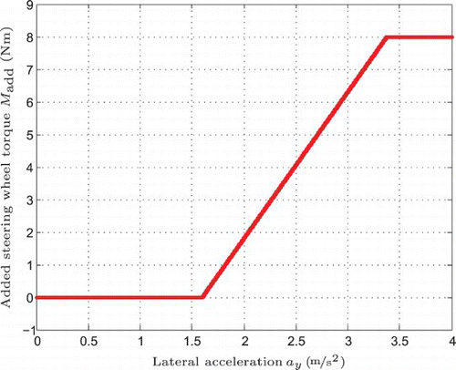
According to the hypothesis of this work, the question is ‘whether drivers of heavy vehicles will perform with more margin of safety to the rollover threshold if the steering wheel torque is decreased or additionally increased at high lateral acceleration’. With the proposed rollover indication algorithm (Section 2), the two strategies could be implemented. The intervention limit and the severity of the intervention (derivative in Figure 3) could also be tuned. The algorithm was implemented in a test vehicle that was equipped with active steering, meaning here free programmable superposition of steering wheel torque (for test vehicle properties, see Section 3.2). The final characteristic for Setting 1 was tuned like shown in Figure 6, the characteristic for Setting 2 had the same shape but a different sign.

Figure 6. Rollover indication characteristic showing the added steering wheel torque over lateral acceleration presented for Setting 1. The intervention begins at a_y=1.6 m/s² and is limited to M_{add, max}=8 N m.

3.1 Test drivers

The driver levels are defined according to:

• (A) Professional test drivers in vehicle dynamics development

• (B) Test engineers in vehicle dynamics development

• (C) Test engineers in chassis development

• (D) Other drivers with driving licence for heavy vehicles

For the present test, drivers of the categories B, C and D were utilised. Since the experiment was divided into two parts because of the different sign of the intervention, the test drivers were divided into two groups, one driving Setting 1 against the reference, and the other driving Setting 2 against the reference. There were in all 33 test drivers divided into the above named two groups. At the end, 27 of them were evaluated since for six of them problems occurred like failure of the active steering system or measuring equipment, or that the drivers chose such a low cornering speed so that they never came up to the lateral acceleration range of intervention.

3.2 Test vehicle

The test vehicle was a series production Scania tractor from 2010 (see Table 1).

Table 1.  Test vehicle properties.

Manufacturer	Scania
Type	R730
Axle configuration	4×2
Wheelbase	3.7 m
Total weight	15.1 t
Axle load distribution	51% front; 49% rear
Active steering	Electric torque overlay (in addition to HPS)

The special feature of this truck was an additional electric power steering (EPS) which worked in cooperation with the series hydraulic power steering (HPS). However, the EPS enabled free programmable additional torque which exceeds the passive HPS.

The truck normally works as a tractor in a semi-trailer–tractor combination. Here, only the tractor was loaded with a frame with extra weight to reach a realistic axle load distribution. There were several reasons for this configuration: on the one hand there were practical constraints; on the other hand the test was performed on a hilly test track and the research question was the vehicle speed chosen by the driver, not given by external constraints like vehicle power and load. If the vehicle speed is limited by external constraints and not by the driver, it will hardly be possible to evaluate the outcomes of the experiment. Even with a powerful engine a tractor–semi-trailer combination reaches its longitudinal acceleration limit quite easily uphill.

3.3 Test track

The experiment was performed on a closed test track. The track that the drivers were asked to drive was similar to a country road with some winding sections, some nearly straight parts and some hairpin bends. Every lap was 7.6 km long and contained 12 bends that forced the driver to slow down to avoid rollover and thereby could be evaluated for this investigation. Ten of these bends were qualified for evaluation. Here, the drivers could choose the vehicle speed on their own irrespectively of other traffic.

According to Schmidt,[16] haptic signals are easiest to detect when the steering activity is low like on narrow roads or in smooth bends. Therefore, the different characteristics of bends on the test track should enable the driver to detect the artificial feedback (conscious or unconscious) and adapt their driving style according to their perception.

3.4 Test procedure

The experiment was performed in Sweden in November, December and January and after 5 pm on each test day. This means that the experiment was performed in darkness and in general on wet or snowy road conditions. These were on the one hand in general adverse conditions; on the other hand, these conditions represent situations where the driver relies on the vehicle and predominantly uses the non-visual feedback.

The drivers were instructed to drive the tractor (equipped with extra load) according to their own style of driving. They knew about active steering being installed in the test vehicle but according to the instruction ‘the purpose of driving was to collect representative driving data with different drivers’. The cockpit including the tachometer was inactive, meaning black, so the drivers had to estimate the vehicle speed by their own perception. Each driver completed 10 laps at a time.

The steering feel modification system was enabled or disabled randomly from lap to lap but consistently for each lap. Bends with another vehicle ahead were discarded with the help of a protocol. The test leader was a passenger in the vehicle to operate the measurement equipment and take notes for the protocol.

3.5 Measurements

For measuring data, the on-board sensors of the test vehicle were used. Vehicle speed, vehicle driving distance, lateral acceleration and yaw rate were measured with a sampling frequency of 1–100 Hz depending on the signal frequency on the Controller Area Network (CAN) bus. The bends were defined in advance by travelled distance along the test track. A pre-test had shown that this method worked properly.

4. Evaluation

For the evaluation, the lateral acceleration log over each curve was extracted. From this a maximum value a_{y, max} and a mean value were calculated for each curve and each driver. In the best case this could theoretically have resulted in a total of 3300 mean and maximum values. For the evaluation around 15% of data was discarded because of disturbances.

The hypothesis of this investigation is that the drivers’ behaviour can be influenced by means of manipulated steering feel. This hypothesis will be tested with drivers of heavy vehicles who are expected to perform with more safety margin to the rollover threshold if the steering wheel torque is decreased or additionally increased at high lateral acceleration. According to Section 2.2 there is no intervention at all up to .

This means that a change of driver behaviour below this limit can neither be reasoned by this functionality nor is it of interest for the investigation. According to Buschardt [14] the JND is situated around 0.5 N m steering wheel torque in a passenger car for 50% of the drivers. The same steering wheel rim force is reached at by the functionality. Therefore, an evaluation window was chosen that began at and covered all measurements above that value. The reason for the difference between start of intervention and lower limit of evaluation window originates from the friction in the steering column. Below these limits there is no risk for rollover accidents due to lateral acceleration that could occur because of too high vehicle speed. The real rollover limit for heavy trucks is situated in the interval of . Ground inclination or extreme crosswind is, of course, not taken into consideration. Naturally, this limit is chosen arbitrarily but moving the limit up or down does not affect the results significantly.

4.1 Normal distributed population

Many statistical methods used for analysing whether two samples differ from each other require normal distributed populations for a stable analysis.

The Shapiro–Wilk test is a powerful test to show whether a sample originates from a normal distributed population. However, it is sensitive for ties, i.e. double or multiple existing ranks of samples. In the present investigation, the on-board sensors of a series truck were used and read via CAN bus which increased the risk for rounded (discrete) and therefore subsequently doubled values.

The Kolmogorow–Smirnow test (KS-test) enables us to test whether two probability distributions match each other by evaluating samples. The test offers high stability; however, it does not separate particularly accurately, i.e. the power of the test is low.[17] Therefore, the further developed variant, the Kolmogorow–Smirnow–Lilliefors test,[18] which is specially optimised for the comparison to normal distributions, was used to analyse whether the populations were normal distributed.

However, both tests indicated that the populations were not normally distributed.

4.2 Drift detection

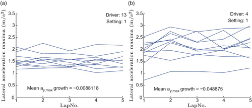
When driving several laps on a test track, the driver becomes familiar with the track. Therefore, it can be expected that the cornering strategy is adapted over several laps. However, in this test case the drivers were used to the test track because of their daily work. Nevertheless, to detect a possible drift for each bend and each driver the maximum and mean lateral acceleration were plotted. Figure 7(a) shows the mean values for each bend (each line represents one bend) for a driver who performs very evenly, with the MSF system enabled. Figure 8(b) shows the maximum values for each bend for a driver who performs more unevenly, also with enabled MSF system. However, the evenness of the plots depends mainly on the driver, not on the MSF system. The mean growth of maximum and mean values was calculated for each driver over all bends by means of the inclination of a line of best fit. This was done for five laps, once with the system enabled and once disabled. The most extreme change was 0.125 and −0.188 while the average of these values over all drivers lay between −0.0164 and 0.0351. Disabling the first lap (understanding it as the ‘learning lap’) does not influence the results significantly. This is interpreted as no indication of any learning effect.

Figure 7. Example plots for two drivers for possible drift detection in mean acceleration over the driver's laps. Every line represents a certain bend: (a) smooth driving and (b) uneven driving.

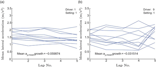
Figure 8. Example plots for two drivers for possible drift detection in maximum acceleration over the driver's laps. Every line represents a certain bend: (a) smooth driving and (b) uneven driving.

4.3 Kernel density estimation

The populations are visualised by means of the kernel density estimation which outputs the distribution function continuously. The distribution function is calculated separately for the laps driven with the reference and those with enabled system (Settings 1 and 2). To calculate comparable functions the density estimate has to be evaluated at similar values. According to the -rule the fragmentation of the estimation interval should be below the root of the number of values in the sample. This leads here to a fragmentation of on the interval [0, 4] for the mean lateral acceleration and a fragmentation of on the interval [0, 5] for the maximum lateral acceleration since every sample consisted of around 750 values inside these intervals. Figure 9(a) shows the kernel density estimation for the lateral acceleration averages for Setting 1 and its reference. The average values are more sensitive to driver failures which can arise while cornering – especially when driving in the dark and on uncertain road conditions (snow). Moreover, the beginning and the end of the bend with lateral acceleration near zero pull the average down without increasing the information content. Nevertheless, the most important section is the lateral acceleration interval between 2.0 and where a decrease of entities at high acceleration can be seen. The same characteristic, even more distinct, is visible in Figure 9(b) which shows the kernel density estimation for the lateral acceleration maxima for the reference and Setting 1. The decrease of entities at high acceleration (for maxima this is the interval between 3 and 5 m/s²) is obvious and marked as a blue area. Concurrently, an increase of entities from reference to Setting 1 at medium high lateral acceleration (interval between 2 and , marked as red area) indicates that the drivers who previously drove near the limit decreased the vehicle speed and therewith the maximum lateral acceleration. The results from Setting 2 do not show a similar affect on the drivers.

Figure 9. Setting 1 kernel density estimation and its reference calculated from the histogram data (10 curves, all drivers). The significance statement origins from Table 2: (a) absolute lateral acceleration: AVERAGES. (b) Absolute lateral acceleration: MAXIMA.

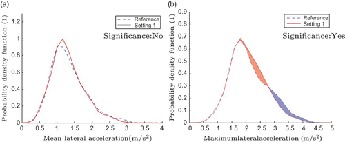
Table 2.  Significance for tests on different populations, each setting against its reference taking the samples>1.7 m/s² into consideration (p-value).

	Maxima		Averages
Ref. vs.	Setting 1	Setting 2	Setting 1	Setting 2
F-test	p=0.08%	p=61.0%	p=4.72%	p=78.5%
t-Test	p=0.84%	p=50.1%	p=43.5%	p=86.1%
U-test	p=5.38%	p=30.0%	p=89.2%	p=56.3%
KS-test	p=1.59%	p=33.5%	p=84.0%	p=77.3%

4.4 Statistic significant differences

There are several possibilities for calculating whether there are statistic significant differences between the estimated populations the samples come from.

The results of the statistical evaluation over all drivers are summarised in Table 2. The significance level is 5%; however, the calculated p-value is given, i.e. a p-value below 5% means that the runs with this setting differ significantly from its references. A driver individual evaluation gave no results because of too few observations for each driver. The results show explicitly that the lateral acceleration maxima for Setting 1 differ from their reference. For the averages and Setting 2 there are no clear differences. This coincides with the kernel density estimation graphs in Figures 9 and 10.

Figure 10. Setting 2 kernel density estimation and its reference calculated from the histogram data (10 curves, all drivers). The significance statement origins from Table 2: (a) absolute lateral acceleration: AVERAGES. (b) Absolute lateral acceleration: MAXIMA.

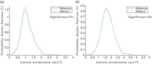
Figure 9(b) shows clearly the two calculated distribution functions from the measuring data. In the lower part, i.e. below of a lateral acceleration of 2 m/s², there is hardly any difference between the two distribution functions. Taking this lower part into consideration when comparing the functions does not provide any more information but increases the noise. To give a complete picture of the measured data, the results of the above performed statistic tests are shown in Table 3.

Table 3.  Complement to Table 2: significance for tests on different populations over full a_y-range.

	Maxima		Averages
Ref. vs.	Setting 1	Setting 2	Setting 1	Setting 2
F-test	p=0.47%	p=69.3%	p=3.97%	p=19.7%
t-Test	p=7.69%	p=99.8%	p=27.4%	p=86.8%
U-test	p=31.9%	p=86.0%	p=60.4%	p=99.4%
KS-test	p=7.52%	p=87.8%	p=73.2%	p=91.3%

Table 2 shows different test results. The aim of this table is to show that the differences that can be seen in Figure 9(b) are significant – independently of the test method used. An overview of the test methods and the particularities in this case follow:

The F-test gives a confidence for two samples coming from different normal distributed populations that differ in their variance.

The t-test gives a confidence for two samples coming from different normal distributed populations that differ in their mean value, and is normally used after a positive F-test. However, in a complex test procedure it is worth performing the t-test as long as it is not the only test on which the conclusions are based.

In spite of the fact that both F-test and t-test require normal distributed populations, which is not the case in this study, both tests were performed to find hints for different driver behaviour with enabled and disabled system. Moreover, since the number of samples is over 50, the requirement of a normal distributed population becomes increasingly weak because of the central limit theorem.[19] Thus, the test results will still be significant.

The χ² test of independence can distinguish two populations. However, it always needs pairs of samples. In this experiment, this means that, for every sample for a certain driver in a certain curve, one sample with enabled system must be compared with a corresponding sample with disabled system. But in the present data set there are several drivings with enabled as well as with disabled system available and they cannot be logically paired. Moreover, for some bends the data are not available because of another vehicle ahead. This situation makes it impossible to decide whether the driver chooses the vehicle speed himself or whether the vehicle's speed is determined by the vehicle driving ahead. One possibility was, of course, to calculate the mean values for each driver; however, this reduces the variance of the data and consequently the content of information. Moreover, the lateral acceleration had to be divided into classes for this test which also reduces the variance of data.

The Wilcoxon–Mann–Whitney test [20] (also called Mann–Whitney–U test, here only U-test) assesses whether one of the two samples of independent observations tends to have larger values than the other. The number of entities in the samples is not required to be the same, which makes this test appropriate to the present evaluation. The test is performed by comparing the calculated ranksums of the samples, i.e. it determines differences in the mean values. The ranksums will only differ significantly if the samples are from different populations.

The previously mentioned KS-test [21] assesses the difference between the estimated population of the samples and another population where the other population can be normally distributed (see above) or have another distribution, represented by other samples. Hence, it can also be used to distinguish between the laps with enabled system from the laps with disabled system. Even here the disadvantage of the relative low power of this test used with ranking scaled not normally distributed populations, must be observed.

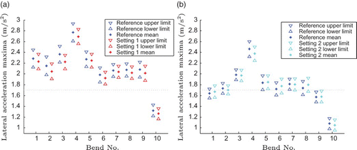
4.5 Bend individual differences

The results in detail are summarised in Table 4. The table shows the differences of mean lateral acceleration maxima and averages for each bend over all drivers. In the bottom line the mean value of each column is calculated, i.e. all drivers that drove Setting 1, take all bends in general with a 3.16% decreased maximum lateral acceleration.

Table 4.  Mean differences to reference in maximum and averaged lateral acceleration in each bend.

	Maxima		Averages
Bend	Setting 1	Setting 2	Setting 1	Setting 2
1	2.42%	−2.04%	2.19%	−2.59%
2	4.78%	1.56%	4.81%	0.85%
3	6.13%	0.63%	3.22%	−1.72%
4	2.86%	3.48%	3.31%	2.24%
5	1.15%	−0.54%	3.13%	−0.84%
6	3.00%	−3.15%	2.83%	−2.26%
7	1.09%	0.21%	−0.86%	−0.30%
8	2.40%	−3.50%	1.15%	−2.49%
9	3.29%	−0.58%	2.19%	−0.04%
10	4.45%	2.48%	2.70%	2.57%
Mean	3.16%	−0.15%	2.47%	−0.46%

This is a quite small difference, which can also be seen in Figure 11. These figures show the 95% confidence intervals of the maximum lateral acceleration over each curve for all drivers. In Figure 11(a) the intervals have a directed offset to a lower lateral acceleration maximum for Setting 1 against its reference. Despite this, the intervals intersect considerably, so this plot shows no significant differences for individual bends. In the same way Figure 11(b) shows intersecting intervals for Setting 2 and its reference. Moreover, the directions of the offsets change randomly. Both plots coincide with the previous findings. Anyway, the differences seem to be very small and cannot be visualised for individual bends.

Figure 11. Differences of maximum lateral acceleration with confidence intervals over bends: (a) Setting 1 against its reference. (b) Setting 2 against its reference.

5. Discussion and conclusions

5.1 Discussion

The hypothesis for this work was that drivers of heavy vehicles will perform with more margin of safety to the rollover threshold if the steering feel is manipulated by means of decreased or additionally increased steering wheel torque at high lateral acceleration. To prove the hypothesis, 33 test drivers (whereof 27 completed, 10 evaluable laps each) took part in an experiment, driving a truck on a test track with 10 significant bends. Five laps were driven with an unmodified vehicle as reference. Five laps were driven with a MSF system – for 15 test drivers an ice-patch-like setting was chosen, for 12 test drivers a lane-keeping-like setting. The evaluation was performed by comparing the distributions of all lateral acceleration average and maximum values measured in each curve. The comparison was done by several statistic methods and the results are shown in Table 2. Additionally, for the measurements of the references, Setting 1 and Setting 2, the distribution functions were calculated by means of kernel density estimation and plotted in Figures 9(b) and 10(b), respectively. Figure 9(b) illustrates the changes of driver behaviour from the upper lateral acceleration range to the midrange.

The driving conditions in this experiment (darkness and wet or snowy road conditions) do not represent all driving conditions. Especially the ‘ice-patch setting’ (Setting 1) will probably be understood differently in summertime; however, even in summertime unexpected slippery road conditions can occur. With the present results, it is not easy to estimate how the drivers will react on summertime road conditions. One limitation is the fact that not all drivers gained experience with driving on slippery surfaces. In certain countries, drivers will not have had to drive on snow-covered roads, for example. Moreover, the tests for Setting 2 were only carried out in snowy road conditions. The results in Figures 10(b) and 11(b) show that the drivers chose a very careful driving style from the beginning and only partially reached the range of intervention. This means that the explanatory power of the tests with Setting 2 is limited.

The test vehicle was a tractor with extra load on the rear axle but without a semi-trailer. In this kind of vehicle a rollover accident is hardly possible. Most drivers can be expected to be aware of this fact, which may influence their driving style. Perhaps the reference lateral acceleration was set at a lower level when driving with a tractor–semi-trailer combination. However, this does not influence the difference by means of manipulated steering feel.

Some drivers complained about a non-linear steering feel – perhaps it would be better to remove the deadband and adapt the slope? Or replace the characteristic by a quadratic function? However, maybe a linear slope would not be experienced distinctly enough as a warning but only as a higher self-aligning torque. In the same way, a quadratic function could be experienced as non-linear – perhaps even worse.

The change in driving behaviour cannot be shown for single drivers, probably due to too few samples – at maximum 100 samples for each driver, i.e. 50 samples for reference against 50 samples for one setting. Moreover, the differences between different drivings of the same bend by the same driver can differ quite substantially (see Figures 8 and 7).

The central limit theorem (Section 4.4) is only valid for independent random variables – the measured values here, the lateral acceleration over a certain test track, are not really random but track dependent and possibly dependent on other variables, too. Contrariwise, especially the t-test is known to be quite stable even with non-normal distributed samples.[22] Therefore, especially for the window analysis of the upper part of lateral acceleration where the sample distribution differs definitely from normal distribution, the non-parametric tests are even more important.

5.2 Conclusion

The statistical evaluation of the experimental results points out that the driver behaviour with enabled system with Setting 1 differs from when driving without the system (Table 2). The characteristic averaged lateral acceleration values show that the drivers choose a midrange cornering speed instead of a high cornering speed (Figure 9(b)). The drivers choose a vehicle speed which leads to a larger safety margin for rollover when the system is activated. Table 4 shows the percentaged decrease of lateral acceleration. However, some drivers complained about the steering feel, which means that the present system cannot be applied directly in a production vehicle.

For future work it can be concluded that the driver behaviour in general can be influenced by tightly focussed steering feel manipulation. Combinations with other systems may increase the collective effectivity of the systems, e.g. driver skill detection [23] and/or a more detailed detection of the single driver's JND. Especially in heavy trucks where the same driver operates the vehicle over many hours, a higher adaptation and personalisation could be realised. The change in driver behaviour indicates future potential for this kind of personalised driver assistance systems.

Acknowledgements

We wish to thank Tom Nyström and posthumously Rickard Lyberger at Scania. Moreover, Annika Stensson Trigell, Daniel Wanner and Johannes Edrén at KTH Vehicle Dynamics and all test drivers for their support during the course of this work.

Funding

The authors are pleased to acknowledge the financial support of Scania and FFI (Swedish Strategic Vehicle Research and Innovation Program).

Notes

1. The JND is the smallest difference between two stimuli which a person can feel. The JND can vary between human beings. The absolute threshold is a special case of the JND where the comparative stimulus is equal to zero.

References

- U.S. Department of Transportation. Large Bus and Truck Crash Facts 2007. FMCSA-RRA-09-029, edition; 2009.
- Chu D-F. Rollover prevention for vehicles with elevated CG using active control. Proceedings of 10th international symposium on advanced vehicle control; Loughborough, UK; 2010.
- Imine H. Identification of heavy vehicle parameters and steering control for rollover prevention. Proceedings of the 22nd symposium of the international association for vehicle system dynamics; Manchester; 2011.
- Chen S-K, Moshchuk N, Nardi F, Ryu J. Vehicle rollover avoidance. IEEE Control Syst. 2010;30:70–85. doi: 10.1109/MCS.2010.937004
- Katzourakis DI, Velenis E, Holweg E, Happee R. Haptic steering support when driving at the tires’ cornering limits. Proceedings of 11th international symposium on advanced vehicle control; Seoul; 2012.
- Katzourakis DI. Driver steering support interfaces near the vehicle's handling limits [PhD thesis]. The Netherlands: TU Delft; 2012.
- Lin RC, Cebon D, Cole DJ. Optimal roll control of a single-unit lorry. Proc Inst Mech Eng Part D: J Automob Eng. 2005;210(1):45–54.
- Cho W, Yoon J, Kim J, Hur J, Yi K. An investigation into unified chassis control scheme for optimised vehicle stability and manoeuvrability. Veh Syst Dyn. 2008;46:87–105. doi: 10.1080/00423110701882330
- Gáspár P, Szászi I, Bokor J. Rollover stability control in steer-by-wire vehicles based on an LPV method. Int J Heavy Veh Syst. 2006;13(1/2):125–143. doi: 10.1504/IJHVS.2006.009121
- Winkler C, Fancher P, Ervin R. Intelligent systems for aiding the truck driver in vehicle control. SAE technical paper series, reprinted from: IV: vehicle navigation systems and advanced controls (SAE 1999-01-1301); 1999.
- Cheng C, Cebon D. Improving roll stability of articulated heavy vehicles using active semi-trailer steering. Veh Syst Dyn. 2008;46:373–388. doi: 10.1080/00423110801958576
- Futterer S, Gerdes M, Niewels F, Ziegler P. Rollover mitigation for light commercial vehicles combining active brake and active steering intervention. VDI Berichte. 2007;2000:721–733.
- Buld S, Krüger H-P. Wirkung von Assistenz und Automation auf Fahrerzustand und Fahrsicherheit. Final report of the project EMPHASIS, Würzburg: Interdisziplinäres Zentrum für Verkehrswissenschaften; 2002.
- Buschardt B. Synthetische Lenkmomente [PhD thesis]. Berlin: Technical University; 2003.
- Pacejka HB. Tyre and vehicle dynamics. Oxford: Butterworth-Heinemann; 2006.
- Schmidt G. Wann spürt der Fahrer überhaupt? VDI-Berichte. 2007; 2015:15–27.
- Yap BW, Sim CH. Comparisons of various types of normality tests. J Stat Comput Simul. 2011;81(12): 2141–2155. doi: 10.1080/00949655.2010.520163
- Lilliefors HW. On the Kolmogorov–Smirnov test for normality with mean and variance unknown. J Am Stat Assoc. 1967;62:534–544. doi: 10.1080/01621459.1967.10482916
- Stevens J. Intermediate statistics. A modern approach. Mahwah, NJ: Erlbaum; 1999.
- Stokes ME, Davis CS, Koch GG. Categorical data analysis using the SAS system. 2nd ed. Cary, NC: SAS Institute Inc.; 2000.
- Feldman RM, Valdez-Flores C. Applied probability and stochastics. 2nd ed. Heidelberg: Springer; 1995.
- Benesch T. Schlüsselkonzepte zur Statistik. Heidelberg: Springer Verlag; 2013.
- Erséus A, Trigell AS, Drugge L. Methodology for finding parameters related to path tracking skill applied on a dlc test in a moving base driving simulator. Int J Veh Auton Syst. 2013;11(1):1–21. doi: 10.1504/IJVAS.2013.052271