Measurement and mathematical model of a driver's intermittent compensatory steering control

Abstract

The compensatory (feedback) component of a human driver's steering control is examined. In particular, the effect of the cognitive process is studied. Model predictive control theory is used to implement models of intermittency in cognitive processing. Experiments using a fixed-base driving simulator with periodic occlusion of the visual display are used to reveal the nature of the driver's steering behaviour. An intermittent serial-ballistic control strategy is found to match the measured behaviour better than intermittent zero-order hold or continuous control. The findings may enable some insight to driver-vehicle interaction and vehicle handling qualities.

Keywords:

• control
• robust control
• driver behaviour
• driving simulator
• driver-vehicle systems
• handling
• objective evaluation
• steering behaviour

1. Introduction

The aim of the work described in this paper is to improve theoretical understanding of human steering control, with a view to enabling the development of mathematical models that can simulate driver-vehicle dynamic behaviour and provide insight to subjective handling qualities. The task of driving a car is often decomposed into two or three levels of control. Donges [1] and Timings and Cole [2] considered the driver's task as a superposition of an open-loop feedforward control action, replaying steering actions learnt over many previous manoeuvres, and closed-loop feedback control, which compensates for internal and external disturbances and uncertainties. The present paper focuses on closed-loop feedback steering control, which will be termed ‘compensatory control’.

The three main functions of the human driver in performing compensatory steering control can be regarded as perception, cognition, and response (or action). This paper concentrates on identifying and modelling aspects of the driver's cognition in performing compensatory control.

Craik [3] was one of the first to propose the hypothesis that cognitive control operates intermittently rather than continuously, generating open-loop ‘ballistic’ movements. Birmingham and Taylor,[4] Elkind,[5] and McRuer and Krendel [6,7] also noticed the existence of intermittent control. Slifkin et al. [8] investigated the effect of intermittency on the ability of subjects to produce a target force. They found that the smallest interval over which visual information can be processed and used to make control decisions, know as the ‘psychological refractory period’ was approximately 150 ms. This is consistent with Larsen et al. [9] who reported that motion processing in the central nervous system can take around 150–300 ms.

The psychological refractory period is also apparent when two separate choice-response tasks are performed concurrently, because responses to one or both tasks can be delayed. This effect can occur even if the two tasks being performed do not share the same input and output channels. The effect is described by Pashler [10] and Ruthruff et al.,[11] and the period is estimated by Navas and Stark [12] as being 150–250 ms. It has been proposed [10,13,14] that the effect is due to a ‘central bottleneck’ in the processing system, so that central operations such as response selection can only take place on one task at a time. It seems plausible that restricting the cognitive capacity available for driving by introducing a secondary task may lead to a greater intermittency in compensatory steering control.

Gawthrop et al. [15] proposed models of intermittent control driven both by a regular clock cycle as well as being ‘event-driven’, that is, reacting to stimuli. Their proposed model of intermittent control is said to be able to ‘masquerade as continuous control’, hence explaining the ability of continuous control models to fit experimental data in some situations.

Roy et al. [16] provided a brief investigation of intermittency in driver steering control using model predictive control (MPC), making use of the first part of the MPC solution over the intermittency period. Simulation results were compared to existing published data for a lane change manoeuvre and it was concluded that ‘intermittent control behaviour is a possibility for human driver steering control without a dramatic change in the dynamics of the closed-loop system’. This observation is consistent with the idea that intermittent control can masquerade as continuous control.[15]

More recently de Kamp et al. [17] devised and performed experiments specifically to identify the refractory period in sustained visuo-manual control of 0th, 1^st, and 2nd order systems. They found that the control action could be interpreted as intermittent in nature, with the period tending to increase with the order of the system: 150–300 ms for 0th order; 250–650 ms for 2nd order.

This paper describes work to assemble and identify a mathematical model of compensatory steering control including intermittency. A particular feature of the work is the use of periodic visual occlusion in driving simulator experiments to aid identification of the open-loop control strategy employed in intermittent control. A realistic model of compensatory steering control may ultimately be helpful in understanding subjective vehicle handling quality. It may be possible, for example, to relate subjective handling quality to the nature of the trade-off between path following performance and secondary task performance. A vehicle that can be steered accurately whilst the driver devotes less cognitive resource to the steering task might be regarded as having desirable handling behaviour.[2] The present work is concerned with intermittency caused by the refractory period and the central bottleneck when input or output resources are not shared, such as a visual/manual driving task combined with a listening/speaking task. However, it should be borne in mind that significant extra delay can occur when tasks share input or output resources. For example, driving combined with operating a keypad both involve vision and manual resources.

In the next section of the paper, various hypothetical cognitive processing strategies are described. In Section 3, an MPC approach is used to represent these strategies mathematically. A parameter study is presented in Section 4. Driving simulator experiments to provide data for identifying the mathematical models are described in Section 5. The models are identified and validated using the experiment data in Section 6. Conclusions are presented in the final section of the paper.

2. Hypotheses for the cognitive process during compensatory control

2.1. Intermittent control and secondary task

Gawthrop et al. [15] propose various hypothetical models of intermittent control of a single task. In this section these models are adapted to include a secondary task.

Figure 1 shows the scheduling of two cognitive tasks: the primary task is compensatory steering control and the secondary task is some other task sharing the same cognitive resource. The central bottleneck hypothesis suggests that the cognitive parts of these two tasks cannot be performed simultaneously. At the very left end of the diagram the states of the vehicle are received from the sensory centres of the brain. There is then some cognitive activity that occupies a finite time (the primary task time τ_pri), then a control signal is sent to the neuromuscular system (NMS). If there is a secondary task then cognitive resource is also devoted to this task (secondary task time) before the states of the vehicle are measured again. The time between outputs of the primary task is the control update time (τ_ctrl), equal to the sum of the primary and secondary task times. In the absence of a secondary task, the primary task time equals the control update time.

Figure 1. Hypothesised scheduling of two tasks through a central bottleneck.

If the update time is sufficiently small then the control actions of the primary and secondary tasks might be indistinguishable from (or ‘masquerading as’ [15]) two independent continuously running (CR) controllers operating on each task separately. However, an intermittent control action might be more representative of human control. One possibility is that the control action is held constant between updates (zero-order hold, ZOH). Another possibility is that the control action is varying and open-loop between updates (serial ballistic hold, SBH).

Gawthrop et al. [15] considered a further feature of the control, which might arise from the human's limited ability to detect changes in response (perception threshold). Thus, the control action might not be updated until the errors being controlled have exceeded a threshold (an event trigger, ET). The threshold might be set by sensory perception limits, or by the driver's motivation to minimise path following errors. Table 1 summarises the cognitive control models examined in this study.

Table 1. Summary of cognitive control models.

Running	Hold	Trigger	Acronym
Continuous	None	None	CR
Continuous	None	Event	CR-ET
Intermittent	Zero order	None	ZOH
Intermittent	Zero order	Event	ZOH-ET
Intermittent	Serial ballistic	None	SBH
Intermittent	Serial ballistic	Event	SBH-ET

Figure 2, following [15], depicts the operation of each controller. The upper graph in each subfigure shows a representative lateral path following error y; the primary task of the cognitive controller is to minimise this error. The lower graph in each subfigure depicts the output θ_com from the primary task of the cognitive controller. The rectangle below this figure indicates the division of cognitive resource between the primary task and a secondary task.

Figure 2. Models of cognitive control for a primary task: (a) CR; (b) CR-ET; (c) ZOH; (d) ZOH, event triggered; (e) SBH; (f) SBH-ET. ‘1’ and ‘2’ denote hypothesised division of cognitive resource between primary and secondary tasks. Acknowledgement to [15].

Figure 2(a) shows the CR controller without a secondary task. The update time is very short compared to the dynamics of the system and thus the control action is effectively continuous. Figure 2(b) shows the continuous-running controller with an event trigger (CR-ET). The controller output for the primary task is zero whenever the path following error is less than the threshold value y_thresh. Figure 2(c) shows an intermittent controller with a secondary task. The controller output changes at the end of the primary task cognitive activity and is then held constant (ZOH) until the end of the next period of primary task cognitive activity. The effect of an ET is shown in Figure 2(d). The primary task activity only takes place when the threshold is exceeded. Otherwise all of the cognitive activity is devoted to the secondary task. Replacing the ZOH with a SBH gives the behaviours shown in Figure 2(e) and 2(f).

2.2. Periodic occlusion of vision

The key difference between the continuous running, intermittent ZOH and intermittent SBH controllers described in the previous section is the nature of the controller output when the cognitive resource is switched to the secondary task. An important objective of the work in this paper is to determine the nature of this control output. Driving simulator experiments have been performed with a secondary task and the results of these will be reported in a future paper; preliminary results can be found in [18]. There is a difficulty in identifying from these experiments the open-loop control action between control updates because it cannot be determined exactly when the cognitive resource is switching between the primary and secondary tasks. Therefore, a visual occlusion experiment was devised to allow easier identification of the open-loop control action between updates.

Experiments were performed on a fixed-base driving simulator in which vision was the only sensory measurement channel by which the driver obtained information about the state of the vehicle (aside from proprioceptive measurements of the steering input). The driver's objective was to steer the vehicle along a straight path whilst subjected to random side force and yaw moment disturbances with zero mean. The effect of a secondary task on the steering (primary) task was imitated by periodic occlusion of the visual feedback to the driver. The experiment results are described in later sections of the paper.

Figure 3 shows the hypothesised control behaviours for a primary task with periods of vision occlusion. For the continuous-running controllers (CR and CR-ET) it is assumed that the controller output is set to zero when the feedback is occluded. In the case of the ZOH hypothesis, it would be natural to assume that the ZOH might be maintained until the end of the occlusion. However, preliminary experiments revealed that this is not realistic behaviour, perhaps because the driver generally cannot predict the duration of the occlusion; it was found that a driver's steering control settles to zero during the occlusion period. Therefore, it is assumed that an update time (refractory period) continues to regulate the open-loop response during occlusion, resulting in a sequence of ZOHs. For the intermittent controllers with serial ballistic hold (SBH and SBH-ET), it is assumed that an optimal open-loop control signal continues to be played during the occlusion, eventually settling to zero. In situations where the target path is not straight or the disturbances on the vehicle have non-zero mean, the settle-to-zero assumption would not be appropriate. In these situations it is likely that the driver would maintain a suitable non-zero steering action during occlusion.

Figure 3. Behaviour of controllers with periodic occlusion. Top: Continuous-running controllers command zero action. Middle and bottom: intermittent controllers implement the remainder of the open-loop control sequence.

3. Mathematical simulation

The driver's steering task is considered as a superposition of feedforward control and feedback (compensatory) control. The simulation presented here represents only the compensatory component of the driver's steering control. Additionally, it is assumed that the vehicle makes only small deviations from a steady operating point, so that the dynamics of the vehicle can be represented by a linear system. A schematic block diagram of the driver and vehicle model is shown in Figure 4. θ_com is the commanded hand wheel (column) angle generated by the cognitive control block. θ_col is the actual hand wheel angle, resulting from adding process noise to θ_com and passing it through a cognitive delay and the NMS. The vehicle model is described in Section 3.1, the driver model is described in Section 3.2, and a parameter study is given in Section 3.3.

Figure 4. Block diagram of the driver-vehicle system model.

3.1. Vehicle model

The vehicle is represented mathematically using the familiar single-track lateral-yaw model with two degrees-of-freedom shown in Figure 5 and Equation (1). The vehicle model and parameter values are based on those reported in [19]. The model represents the linearised dynamics of the nonlinear vehicle about a nominal operating point. External disturbances are a lateral force F_dist and a yaw moment M_dist at the centre of mass. (1) $\left\{\begin{array}{c}\dot{\nu }\\ \ddot{\psi }\\ \dot{y}\\ \dot{\psi }\end{array}\right\}=\left[\begin{array}{cccc}-\frac{C_r+C_f}{MU}& \frac{b{C}_r-a{C}_f}{MU}-U& 0& 0\\ \frac{b{C}_r-a{C}_f}{IU}& -\frac{a^2{C}_f+b^2{C}_r}{IU}& 0& 0\\ 1& 0& 0& U\\ 0& 1& 0& 0\end{array}\right]\left\{\begin{array}{c}v\\ \dot{\psi }\\ y\\ \psi \end{array}\right\}+\left[\begin{array}{ccc}\frac{C_f}{GM}& \frac{1}{M}& 0\\ \frac{a{C}_f}{GI}& 0& \frac{1}{I}\\ 0& 0& 0\\ 0& 0& 0\end{array}\right]\left\{\begin{array}{c}{\theta }_{\mathrm{col}}\\ F_{\mathrm{dist}}\\ M_{\mathrm{dist}}\end{array}\right\}.$(1)

Figure 5. Lateral-yaw ‘bicycle’ model of a car.

The front and rear tyre cornering stiffnesses are set to one of three possible pairs of values, as shown in Table 2, each representing a different dynamic behaviour. The values labelled ‘Base’ represent a passenger car running along a nominally straightline trajectory with tyres operating around zero slip angle. The values labelled ‘US’ represent an understeering vehicle approaching the limit of adhesion where the front axle is nearer to saturation than the rear axle. The values labelled ‘OS’ represent an oversteering vehicle approaching the limit of adhesion where the rear axle is nearer to saturation than the front axle. The centre of mass of this vehicle is further backwards than that of the Base and US vehicles. All three vehicles are stable, but the OS vehicle is close to the limit of stability.

Table 2. Vehicle model parameter values.

Symbol	Parameter	Base	US	OS	Units
Cf	Front axle cornering stiffness	229,240	36,546	41,487	N rad^−1
Cr	Rear axle cornering stiffness	229,240	131,802	36,546	N rad^−1
M	Vehicle mass	1050	1050	1050	kg
I	Vehicle yaw inertia	1500	1500	1500	kg m^2
U	Forward speed	30	30	30	m s^−1
a	Centre of mass to front axle	0.92	0.92	1.16	m
b	Centre of mass to rear axle	1.38	1.38	1.14	m
G	Steering gear ratio	17	17	17	–

The dynamics of the NMS of the driver's arms are represented by a second-order low-pass filter with natural frequency ω_nms and damping ratio ζ_nms.[20] Time delay τ_delay is included, to account for the neuromuscular and sensory systems. The delay is implemented as a shift register.

The force and moment disturbances at the vehicle's centre of mass are filtered by a low-pass second-order Butterworth filter, cut-off frequency f_c. Cognitive and neuromuscular process noise and sensory measurement noise can be added to the simulation as shown in Figure 4.

3.2. Controller

The driver's cognitive control is represented using MPC. For details of MPC, see [21–24]. The ‘plant’ to be controlled is the vehicle and NMS described in Section 3.1. The prediction model is identical to the plant. MPC involves using the state equation and output equation (specified with A, B, C state space matrices) to predict the output of the plant up to a prediction horizon N time steps ahead, as shown in Equations (2) and (3): (2) $\left\{\begin{array}{c}{\mathbf{\text{x}}}_{(k+1)}\\ {\mathbf{\text{x}}}_{(k+2)}\\ ⋮\\ {\mathbf{\text{x}}}_{(k+N)}\end{array}\right\}=\left[\begin{array}{c}\mathbf{\text{A}}\\ {\mathbf{\text{A}}}^2\\ ⋮\\ {\mathbf{\text{A}}}^N\end{array}\right]{\mathbf{x}}_{\left(k\right)}+\left[\begin{array}{cccc}\mathbf{\text{B}}& \mathbf{\text{0}}& \cdots & \mathbf{\text{0}}\\ \mathbf{\text{AB}}& \mathbf{\text{B}}& \cdots & \mathbf{\text{0}}\\ ⋮& ⋮& \ddots & ⋮\\ {\mathbf{\text{A}}}^{N-1}\mathbf{\text{B}}& {\mathbf{\text{A}}}^{N-2}\mathbf{\text{B}}& \cdots & \mathbf{\text{B}}\end{array}\right]\left\{\begin{array}{c}{\theta }_{\mathrm{com}(k)}\\ {\theta }_{\mathrm{com}(k+1)}\\ ⋮\\ {\theta }_{\mathrm{com}(k+N-1)}\end{array}\right\},$(2) (3) $\left\{\begin{array}{c}{\mathbf{\text{y}}}_{(k+1)}\\ {\mathbf{\text{y}}}_{(k+2)}\\ ⋮\\ {\mathbf{\text{y}}}_{(k+N)}\end{array}\right\}=\left[\begin{array}{cccc}\mathbf{\text{C}}& \mathbf{\text{0}}& \cdots & \mathbf{\text{0}}\\ \mathbf{\text{0}}& \mathbf{\text{C}}& \cdots & \mathbf{\text{0}}\\ ⋮& ⋮& \ddots & ⋮\\ \mathbf{\text{0}}& \mathbf{\text{0}}& \cdots & \mathbf{\text{C}}\end{array}\right]\left\{\begin{array}{c}{\mathbf{\text{x}}}_{(k+1)}\\ {\mathbf{\text{x}}}_{(k+2)}\\ ⋮\\ {\mathbf{\text{x}}}_{(k+N)}\end{array}\right\},$(3) where x is the state vector, y is the measurement or output vector, and k is the discrete-time index. An optimal sequence of control actions is calculated that minimises a mean square cost function V of the form: (4) $V_{\left(k\right)}=\sum _{i=1}^N\left(\right|\left|{\mathbf{\text{y}}}_{(k+i)}\right|{|}_{\mathbf{\text{R}}\left(i\right)}^2+\left|\right|{\theta }_{\mathrm{com}(k+i-1)}\left|{|}_{Q\left(i\right)}^2\right),$(4) (5) ${\mathbf{\text{R}}}_{\left(i\right)}=\left[\begin{array}{cccc}{R}_y& 0& 0& 0\\ 0& 0& 0& 0\\ 0& 0& R_{\psi }& 0\\ 0& 0& 0& 0\end{array}\right],$(5) where the first term in the summation is the mean square path following errors, and the second term is the mean square control action. R_y is the weighting on lateral path error (the target path is assumed to be straight), R_ψ is the weighting on heading error and Q is the weighting on commanded steering angle.

In the case of a CR the first element of the optimal control sequence is applied to the plant and the rest of the sequence is discarded. At the next time step of the simulation a new sequence of control actions is calculated and the first of these is applied.

Intermittent control with a SBH can be simulated using MPC by simply using the optimal control sequence until the next update of feedback information, at which point a new optimal control sequence is calculated.[24] In the case of a long occlusion period the control sequence may have settled to zero, otherwise there is likely to be a discontinuity in the control.

To represent intermittent ZOH control, the MPC is formulated slightly differently. The control sequence is assumed to consist of successive ZOHs, the duration of each ZOH equal to the refractory time. The sequence of ZOH controls is delivered to the plant until the next update of feedback information.

Since all of the states of the plant are not in practice directly measurable by the driver, an observer is included to estimate the states from the noisy measurements. The measurements made by the driver are assumed to be the lateral and yaw displacements and velocities of the vehicle. The observer is implemented as a Kalman filter. The validity of such an observer to represent a human driver's estimation process is the subject of related research.[25]

4. Parameter study

The behaviour of the six controllers listed in Table 1 is investigated briefly in this section. The discrete-time simulation time step T_s is 10 ms. The driver time delay τ_delay is 130 ms, comprising 90 ms from the NMS and 40 ms from the sensory system. The prediction horizon N is 400 time steps, which is 4 s. No secondary task or occlusion is included, therefore, the primary task time τ_pri is equal to the update time τ_ctrl. For the ET controllers the lateral displacement threshold y_thresh is initially set to 0.1 m. The complete set of parameter values is given in Table 3.

Table 3. Simulation parameter values.

Symbol	Parameter	Value	Units
Ts	Simulation time step	10	ms
Tend	Simulation duration	30	s
ωnms	NMS natural frequency	5.78	rad s^−1
ζnms	NMS damping ratio	0.44	–
τdelay	NMS plus sensory time delay	130	ms
N	Prediction horizon steps	400	–
Ry	Penalty on lateral path error y	1	–
Rψ	Penalty on yaw angle error ψ	0	–
Q	Penalty on commanded hand wheel angle θcom	1	–
τctrl	Control update time	0.1	s
τpri	Primary task time	0.1	s
ythresh	Threshold on y for event trigger	0.1	m
σF	Lateral force disturbance std. dev.	14	kN
σM	Moment disturbance std. dev.	0	N m
fc	Disturbance low-pass filter frequency	2	Hz

4.1. Response to random lateral force and yaw moment disturbance

In this simulation, the target path is a straight line and random lateral force and yaw moment are applied to the centre of mass of the vehicle. The force and moment disturbances are uncorrelated random white noise signals with the standard deviations given in Table 4. These signals are then modified by the low-pass filters before being applied to the vehicle. Measurement noise and process noise are applied as indicated in Figure 4. Uncorrelated white noise signals are applied to the four measured vehicle states. The variances of the noise signals are determined from typical signal variance values divided by a signal to noise ratio, specified in Table 4.

Table 4. Noise parameter values.

Symbol	Parameter	Value	Units
σF	Force disturbance std. dev. (base/US/OS)	14.0/7.1/4.5	kN
σM	Moment disturbance std. dev. (base/US/OS)	10.0/5.0/3.2	kN m
Ξ	Signal to noise ratio	20	dB
σy	Std. dev. of typical y signal	0.58	m
σdy	Std. dev. of typical dy/dt signal	0.37	m s^−1
σψ	Std. dev. of typical ψ signal	0.07	rad
σdψ	Std. dev. of typical dψ/dt signal	0.33	rad s^−1
σθ	Std. dev. of typical θ signal	0.88	rad

Figure 6 shows the root mean square (RMS) lateral path following error on the vertical axis against primary task time on the horizontal axis. When the primary task time is less than the update time, it is assumed that a secondary task is taking place (see Figure 1). The update time cannot be less than the primary task time. The CR controller is used when the update time and primary task time are 0.01 s (the simulation discrete-time step). The lateral displacement threshold for the ET controllers is 0.1 m. RMS values were calculated from simulated time histories each of 1000 s duration.

Figure 6. RMS lateral path following error against primary task time for various control update times. Controller: circles ZOH, squares ZOH-ET, triangles SBH, crosses SBH-ET.

Looking at all the points corresponding to a primary task time of 0.01 s it can be seen that the RMS path error increases as the update time increases. As the update time increases, the SBH controllers perform better than the ZOH controllers. The effect of the ET and 0.1 m threshold is small compared to the effects of changing the primary task time and update time. Increasing the threshold causes the RMS path error to increase, but only once the threshold approaches the path error (results not shown due to lack of space). The RMS path error also tends to increase as the primary task time increases.

4.2. Response to random disturbances with periodic occlusion of vision

In this simulation, the random disturbances continue to be applied (Table 4) but vision is periodically occluded. The same random disturbance is used for each simulation to allow the time responses of the different controllers to be compared. The update time and primary task time are both set to 0.1 s and the lateral path error threshold is 0.1 m. The simulation time is 1000 s.

Figure 7 shows the simulated effect of occlusion. The upper graph shows the lateral displacement of the vehicle. The centre graph is the commanded hand wheel angle and the bottom graph is the actual hand wheel (column) angle. The difference between the commanded hand wheel angle and the actual hand wheel angle is due to the NMS dynamics. However, in this simulation, because the NMS dynamics are accounted for in the calculation of the optimum commanded hand wheel angle, as described in Section 3.2, the NMS dynamics should not necessarily be regarded as contributing uncertainty and consequent instability. Also note that, since the event threshold is small compared to the lateral path errors, there is little difference between the controllers with and without the ET.

Figure 7. Comparison of path following performance of the controllers running with periodic occlusion. Dashed: CR and CR-ET; Solid: ZOH and ZOH-ET; Dotted: SBH and SBH-ET. Event threshold y_thresh = 0.1 m. The effect of the event threshold is negligible.

The continuous-running controllers (CR and CR-ET) set the commanded hand wheel angle to zero during the occlusion (although the dynamics of the NMS mean that the column angle continues to respond after the onset of occlusion.) The consequence is large lateral displacements of the vehicle.

The intermittent controllers ZOH, ZOH-ET, SBH, and SBH-ET use the sequence of optimal control actions during the occlusion period. As with the continuous-running controllers, these control action sequences are modified by the NMS dynamics before reaching the hand wheel. Although these sequences eventually settle to zero before the end of the occlusion period, their longer duration compared to the continuous-running controllers means that they are more effective in reducing the lateral displacements.

5. Driving simulator experiment

A fixed-base driving simulator [26] was used to collect data to identify and validate the driver models described in the previous section. The three vehicle models in the simulator were identical to those described in Section 3.1 and Table 2. The driver's task was simply to steer the vehicles along a straight path in the presence of the random lateral force and yaw moment disturbances specified in Table 4.

The driving task was performed with normal vision of the oncoming road path, and with periodic visual occlusion of the road path. The periodic visual occlusion comprised vision for 0.4 s followed by occlusion for 2.5 s. The driving simulator had no motion cueing and the steering torque characteristic did not depend on the vehicle states, therefore occluding the vision prevented the driver from sensing any information on the state of the vehicle.

There were six test subjects, details are given in Table 5. The test procedure for each subject and each vehicle consisted of:

1. At least 5 min of practice under the normal driving condition;

2. The normal driving condition experiment for 7.5 min;

3. A break of approximately 10 min;

4. At least 5 min of practice under the occlusion condition;

5. The occlusion condition experiment for 7.5 min.

Table 5. Human test subjects.

Subject	Age/years	Gender	Previous driving simulator experience?	Real driving experience?
1	24	Male	Yes	6 years
2	28	Male	Yes	None
3	26	Male	No	1 year
4	25	Female	No	1 year
5	26	Male	No	None
6	24	Female	No	7 years

The total testing time was approximately 1.5 h for each subject, and subjects often elected to perform the tests over three successive days.

Typical hand wheel angle time histories are shown in Figure 8. The upper plot shows 20 s of response from test subject 1 driving the base vehicle with normal vision. The peak-to-peak steering angle in this plot is about 1 rad. The lower plot shows the response of the same subject in the same vehicle but with periodic occlusion of vision (indicated by the shaded regions at the bottom of the plot). There is a noticeable pattern of steering response that is synchronised with the occlusion cycle, and which often features a nearly constant and small angle towards the end of the occlusion part of the cycle. The peak-to-peak angle is about 2 rad. In the next section of the paper, the measured data is used to identify and validate the models of compensatory steering control.

Figure 8. Typical measured steering wheel angle time histories during (a) normal vision and (b) periodic occlusion.

6. Identification and validation

Parameter values of the CR and SBH compensatory steering controllers were identified using a direct prediction error method. A noise model was identified and used to weight the hand wheel angle prediction error to minimise bias in the estimates of the parameter values. For details of the prediction error method and bias minimisation see [26,27]. A simulation study was undertaken to confirm the operation of the identification and validation procedure, details can be found in [28].

The number of free parameters was limited in order to prevent overfitting of the data. The following model parameters were fixed: measurement and process noise variances (Table 4); NMS natural frequency and damping (Table 3). Since no secondary task was performed during any of the experiments the update time was set equal to the primary task time. The NMS plus sensory time delay τ_delay was identified for all the controllers. For ET controllers the threshold y_thresh was identified. The SBH controllers were only identified with an ET in operation, since an identified threshold value of 0 m would indicate the absence of an ET in the test subject's control action. For the intermittent controllers the control update time τ_ctrl was identified (although this was expected to be unreliable [17]).

The structure of the cost function was slightly different for the CR and SBH controllers. Inspection of the measured data from the periodically occluded driving experiments suggested that the drivers might have used a strategy in which lateral path error was prioritised for the first part of the occlusion period, after which minimising heading error was prioritised. This strategy was implemented in the SBH controllers by adjusting the cost function weights (Equation (5)) along the prediction horizon so that R_ψ = 0 for 1 < i < N_ω and R_y = 0 for N_ω < i < N, where N_ω is the number of time steps along the prediction horizon at which the transition from weighting lateral path error to heading error occurs.

Thus, for the identification of the SBH controllers, parameters R_y, R_ψ and N_ω were identified. For the CR controllers, which set the commanded control action to zero during occlusion, the cost function was assumed to be constant along the prediction horizon with R_ψ set to zero and the value of R_y to be identified. In all cases the weighting Q on commanded hand wheel angle was set to 1.

Half of the measured 7.5 min of data was used for identification and the remaining half was used for validation. The success of the validation was evaluated using the ‘normalised RMS hand wheel angle prediction error’ E defined as: (6) $E=\frac{\mathrm{RMS}({\theta }_{\mathrm{col}.\mathrm{meas}}-{\theta }_{\mathrm{col}})}{\mathrm{RMS}({\theta }_{\mathrm{col}.\mathrm{meas}})},$(6) which is the RMS of the hand wheel angle prediction error divided by the RMS of the measured hand wheel angle θ_col.meas.

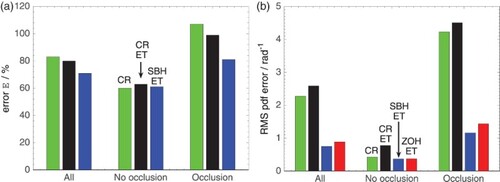
Figure 9(a) compares the prediction error averaged across all the test subjects and test vehicles. For normal vision (no occlusion) the errors are similar. For occluded vision the SBH-ET controller performs better than the continuous-running controllers (CR and CR-ET). The prediction errors are larger than reported in some other driver model identification studies, for example, [29]. However, in such studies it is usually the feedforward steering control behaviour that is of interest, and the compensatory control behaviour is removed by averaging together repeated experiments. In the present study only the compensatory control is investigated.

Figure 9. (a) Normalised RMS hand wheel angle prediction error. (b) RMS hand wheel angle probability density error. Lower values are better.

Figure 10 shows two typical time histories of the measured hand wheel angles along with the corresponding simulated responses of the identified controllers. The upper graph is test subject 4 driving the understeer vehicle with continuous vision. The simulated responses of the three identified controllers are similar to each other; the differences between them are smaller than the differences to the measured response, but note that the simulated responses in the graph do not include a contribution from the noise model. The lower graph is test subject 1 driving the oversteer vehicle with periodically occluded vision. The simulated responses of the CR and CR-ET controllers are indistinguishable because the periodic occlusion ensured that path errors were significantly larger than the drivers’ threshold. The SBH-ET controller seems to match the measured response better than the CR controllers, particularly at the peaks of response.

Figure 10. Typical time histories of hand wheel (column) angle from the experiments and from the identified controllers. (a) US vehicle, subject 4, normal vision and (b) OS vehicle, subject 1, periodic occlusion. The traces for the CR (thin dash) and CR-ET (thick dash) controllers are essentially coincident.

It is interesting to compare the time responses of hand wheel angle generated for the parameter study shown in Figure 7 with the responses of the identified controllers in Figure 10. The random disturbances were the same in each case, but it is clear that the hand wheel angle amplitudes in the parameter study were significantly smaller than in the experiment. This is explained by the weighting on path error in the cost function for the parameter study (Table 3, R_y = 1) being several orders of magnitude higher than the weightings identified from the driving simulator experiment data (see [28] for values).

Another interesting observation is that the CR, ZOH, and SBH controllers in the parameter study (Figure 7) show a much larger difference in response when compared to each other than do the CR, ZOH, and SBH controllers identified from the driving simulator experiments (Figure 10). This is because a single set of parameter values was used in all three controllers in the parameter study, whereas in the experiment parameter values were identified separately for each controller in order to achieve best fit to the measured hand wheel angle (see [28] for values).

Figures 11 shows the measured and simulated hand wheel (column) angle amplitude probability density functions for test subject 4 driving the US vehicle with periodically occluded vision. Parameter values for the ZOH-ET controller were taken from the results of identifying the SBH-ET controller. The figure shows that the SBH-ET controller fits the measured distribution much better than the other controllers. The corresponding comparison for driving with normal vision (not shown) revealed that all the controllers agreed quite well with the measured distribution. The discrepancy between measured and simulated probability density function distributions can be calculated as a RMS of the difference, evaluated across a span of −2 to +2 rad. Figure 9(b) plots these values for the continuous and the intermittent controllers, averaged across all the drivers and vehicles, confirming that the intermittent controllers better represent the measured amplitude distribution.

Figure 11. Probability density function of hand wheel (column) angle from the experiments (US vehicle, subject 4) and from the identified controllers during periodically occluded vision. The traces for the CR and CR-ET controllers are coincident.

The control update time identified for the SBH-ET controller was 136 ms, which is a little below the range of 150–650 ms reported in the literature. The difficulty of identifying this time reliably without using special experimental conditions is noted in [17]. However, the identified time is much longer than the simulation discrete-time step of T_s = 10 ms, and indicates that intermittent control is a more likely hypothesis than continuous control.

The mean value of the identified NMS and sensory time delay τ_delay was 155 ms. This is perhaps longer than other studies in the literature suggest. It is possible that some of this time delay should be allocated to the control update time.

The mean value of the N_ω parameter for the intermittent controllers identified from the occlusion experiments was 215 steps, or 2.15 s. There was no significant difference of this value between the different vehicles, but there were differences between test subjects, ranging from 150 to 350 steps.

The identified lateral path error cost function weights (see [28] for details) were generally larger for the normal driving case compared to the periodic occlusion case. This corresponds to the test subjects placing more emphasis on minimising lateral path error compared to minimising control action during normal driving.

In summary, the results of the identification and validation tend to support the hypothesis that a human driver acts like an intermittent controller, and that a serial ballistic strategy is employed when intermittency or visual occlusion prevents update of the control.

As noted in Section 2.2, an aim of the work was to determine experimentally the nature of the steering control output when the cognitive resource is switched to a secondary task. However, a difficulty was anticipated in identifying the steering control output in such an experiment because it cannot be determined exactly when the cognitive resource is switching between the steering task and secondary task. Therefore, visual occlusion was used to deprive the steering task of sensory information, instead of employing a secondary task.

The use of a fixed-base driving simulator ensured that no other sensory information was available to the driver during the occlusion period. Further work is required to determine whether the model of cognitive behaviour identified from the visual occlusion experiment is representative of driving a real car whilst performing a secondary (listening/speaking) task. In this case the driver would be subjected to continuous motion and haptic feedback as well as visual feedback; it needs to be established whether the undertaking of a secondary listening/speaking task would prevent the driver from processing this sensory information, and whether the open-loop control sequence from the steering task would continue to be played out whilst the cognitive resource is allocated to the secondary task.

A long occlusion time was chosen in this experiment to ensure that all of the driver's open-loop action was played out before vision was restored. In a real driving situation in which a secondary task shares the vision channel it is unlikely that the ratio of occlusion to vision would reach such extreme values as employed in this experiment. Further work could usefully explore smaller ratios of occlusion to vision.

7. Conclusion

A review of the literature in the field of cognitive processing strategies revealed that the concepts of intermittent control and central bottleneck had not been extensively investigated in relation to a vehicle driver's compensatory steering task. It was concluded that further research in this area might ultimately provide insight to subjective vehicle handling qualities.

MPC was used to simulate the cognitive process of a driver performing compensatory steering control along with a secondary task. Several hypotheses [15] were simulated, including continuous control, intermittent control with ZOH, and intermittent control with SBH. In addition, an ET based on a path following error threshold was simulated.

A parameter study revealed that the path following error in the presence of disturbances on the vehicle increases as the control update time increases. The path following error also increases if the control update time is fixed but the primary task time increases (time between measurement and control action). The serial-ballistic controller generated smaller path errors than the ZOH controller for the particular parameter values studied. An ET had little effect on the performance if the threshold was significantly smaller than the path following errors.

Fixed-base driving simulator experiments were performed to provide data for identification and validation of the driver compensatory steering control models. The experiments included periodic occlusion of vision to allow more reliable identification of any open-loop control by the driver.

The continuous-running and serial-ballistic-hold controllers were fitted to the measured data. It was found there was little difference in the prediction accuracy of the two controllers during the normal (no occlusion) driving, but the serial-ballistic-hold controller was significantly better than the CR in predicting the drivers’ compensatory steering action for the periodic visual occlusion condition.

The large differences in performance between the controllers using one set of parameter values in the parameter study were not so apparent when each controller was identified separately using the data from the driving simulator experiment.

Analysis of the amplitude distribution of measured and simulated steering angles suggested that the serial ballistic hold controller was better than a ZOH controller, although the parameter values of the ZOH controllers were not identified directly from the experiments.

The control update time (refractory period) was identified as 138 ms, which is just outside the range reported in the literature, but significantly larger than the 10 ms discrete-time step of the simulation.

For the periodic occlusion experiments, it was found that a cost function penalising lateral path error in the first part of the prediction horizon and heading error in the remaining part of the prediction horizon was better than a cost function penalising only lateral path error.

It is concluded that intermittent control with serial ballistic hold is suitable for representing the driver compensatory steering control behaviour observed in the fixed-base driving experiments. The work adds significantly to the findings of Roy et al.,[16] by focusing on compensatory control, and by performing dedicated experiments to identify a range of models.

Further work is underway to extend the modelling approach to deal with nonlinear vehicle dynamics arising from operation in the saturation region of the tyre characteristic. The work will also be extended to deal with combined steering and longitudinal control.

Disclosure statement

No potential conflict of interest was reported by the authors.

Additional information

Funding

This work was supported by the Engineering and Physical Sciences Research Council [EP/P505445/1]; the Qualcomm European Research Studentship Fund in Technology; and the Lotus F1 Team [RG61664]. Supporting data are available at Cambridge University digital repository: https://www.repository.cam.ac.uk/handle/1810/251180.

References

- Donges E. A two-level model of driver steering behaviour. Hum Factors. 1978;20(6):691–707.
- Timings JP, Cole DJ. Robust lap-time simulation. Proc Inst Mech Eng D J Automob Eng. 2014;228:1200–1216. doi: 10.1177/0954407013516102
- Craik KJ. Theory of the human operator in control systems: the operator as an engineering system. The Br J Psychol. 1947;38(2):56–61.
- Birmingham HP, Taylor FV. A human engineering approach to the design of man-operated continuous control systems. Technical Report NRL-4333. Washington (DC): Naval Research Laboratory; April 1954.
- Elkind JI. Characteristics of simple manual control systems [PhD thesis]. MIT; June 1956.
- McRuer DT, Krendel ES. The human operator as a servo system element: Part I. J Franklin Inst. 1959;267(5):381–403. doi: 10.1016/0016-0032(59)90091-2
- McRuer DT, Krendel ES. The human operator as a servo system element: Part II. J Franklin Inst. 1959;267(6):511–536. doi: 10.1016/0016-0032(59)90072-9
- Slifkin AB, Vaillancourt DE, Newell KM. Intermittency in the control of continuous force production. J Neurophysiol. 2000;84:1708–1718.
- Larsen A, Farrell JE, Bundesen C. Short- and long-range processes in visual apparent movement. Psychol Res. 1983;45:11–18. doi: 10.1007/BF00309348
- Pashler H. Processing stages in overlapping tasks: evidence for a central bottleneck. J Exp Psychol Hum Percept Perform. 1984;10(3):358–377. doi: 10.1037/0096-1523.10.3.358
- Ruthruff E, Pashler HE, Klaassen A. Processing bottlenecks in dual-task performance: structural limitation or strategic development? Psychon Bull Rev. 2001;8(1):73–80. doi: 10.3758/BF03196141
- Navas F, Stark L. Sampling or intermittency in hand control system dynamics. Biophys J. 1968;8(2):252–302. doi: 10.1016/S0006-3495(68)86488-4
- Wickens CD. Multiple resources and mental workload. Hum Factors. 2008;50(3):449–455. doi: 10.1518/001872008X288394
- Sarno KJ, Wickens CD. Role of multiple resources in predicting time-sharing efficiency: evaluation of three workload models in a multiple task setting. Int J Aviat Psychol. 1995;5(1):107–130. doi: 10.1207/s15327108ijap0501_7
- Gawthrop P, Loram I, Lakie M, Gollee H. Intermittent control: a computational theory of human control. Biol Cybern. 2011;104:31–51. doi: 10.1007/s00422-010-0416-4
- Roy R, Micheau P, Bourassa P. Intermittent predictive steering control as an automobile driver model. J Dyn Sys, Meas, Control. 2008; 131(1):014501-014501-6. doi:10.1115/1.3023127.
- van de Kamp C, Gawthrop PJ, Gollee H, Loram ID. Refractoriness in sustained visuo-manual control: is the refractory duration intrinsic or does it depend on external system properties? PLoS Comput Biol. 2013;9(1):e1002843. doi:10.1371/journal.pcbi.1002843.
- Johns T, Cole DJ. A model of driver compensatory steering control incorporating cognitive limitations. Proc. 23rd IAVSD Symposium on the Dynamics of Vehicles on Roads and Tracks; August 2013; Qingdao, China.
- Timings JP, Cole DJ. Minimum manoeuvre time calculation using convex optimisation. J Dyn Syst Meas Control. May 2013;135: 031015, 9p. doi: 10.1115/1.4023400
- Pick AJ, Cole DJ. Dynamic properties of a driver's arms holding a steering wheel. Proc Inst Mech Eng. 2007; 221 Part D:1475–1486.
- Maciejowski JM. Predictive control with constraints. 1st ed. Harlow: Prentice Hall; 2001. 352p.
- Cole DJ, Pick AJ, Odhams AMC. Predictive and linear quadratic methods for potential application to modelling driver steering control. Veh Syst Dyn. 2006;44(3):259–284. doi: 10.1080/00423110500260159
- Keen SD, Cole DJ. Application of time-variant predictive control to modelling driver steering skill. Veh Syst Dyn. 2011;49(4):527–559. doi: 10.1080/00423110903551626
- Johns T, Cole DJ. A model of driver compensatory steering control incorporating cognitive limitations. Proc. 11th International Symposium on Advanced Vehicle Control, AVEC 2012; September 2012; Seoul, South Korea.
- Nash CJ, Cole DJ. Development of a novel model of driver-vehicle steering control incorporating sensory dynamics. Proc. IAVSD Symposium on Dynamics of Vehicles on Roads and Tracks; August 2015; Graz, Austria.
- Odhams AMC, Cole DJ. Identification of preview steering control models using data from a driving simulator and a randomly curved road path. Int J Auton Veh Syst. 2014;12(1):44–64. doi: 10.1504/IJVAS.2014.057863
- Ljung L. System identification: theory for the user. 2nd ed. Upper Saddle River (NJ): Prentice Hall; 1998, 672p.
- Johns T. The effect of cognitive workload on a racing driver's steering and speed control [PhD thesis]. University of Cambridge; January 2014.
- Keen SD, Cole DJ. Bias-free identification of a linear model predictive steering controller from measured driver steering behavior. IEEE Trans Syst Man Cybern B. 2012;42(2):434–443. doi: 10.1109/TSMCB.2011.2167509