Establishment and verification of three-dimensional dynamic model for heavy-haul train–track coupled system

ABSTRACT

For the long heavy-haul train, the basic principles of the inter-vehicle interaction and train–track dynamic interaction are analysed firstly. Based on the theories of train longitudinal dynamics and vehicle–track coupled dynamics, a three-dimensional (3-D) dynamic model of the heavy-haul train–track coupled system is established through a modularised method. Specifically, this model includes the subsystems such as the train control, the vehicle, the wheel–rail relation and the line geometries. And for the calculation of the wheel–rail interaction force under the driving or braking conditions, the large creep phenomenon that may occur within the wheel–rail contact patch is considered. For the coupler and draft gear system, the coupler forces in three directions and the coupler lateral tilt angles in curves are calculated. Then, according to the characteristics of the long heavy-haul train, an efficient solving method is developed to improve the computational efficiency for such a large system. Some basic principles which should be followed in order to meet the requirement of calculation accuracy are determined. Finally, the 3-D train–track coupled model is verified by comparing the calculated results with the running test results. It is indicated that the proposed dynamic model could simulate the dynamic performance of the heavy-haul train well.

KEYWORDS:

• Heavy-haul train
• longitudinal train dynamics
• vehicle–track coupled dynamics
• coupler force

1. Introduction

The long freight train with the larger axle load has been a main technical measure for countries to improve the railway freight volume. A long heavy-haul train can be characterised by its huge number of vehicles, numerous degrees of freedom (DOFs), and the complicated kinematic relations. As the train brakes, there may exist simultaneously the serious longitudinal impulses and the wheel–rail interactions. For a long time, researches on the heavy-haul train dynamics were mainly carried out from three aspects, namely the train longitudinal dynamics, the three-dimensional (3-D) vehicle dynamics and the vehicle–track coupled dynamics.

The emphasis of the typical train longitudinal dynamics is to investigate the train dynamic motions in the direction of track. Generally, the train can be described as a multi-mass system only with the longitudinal motions. The total mass of a locomotive or a freight wagon is lumped to its centre of mass. The classical model and modelling method can be traced back to the 1960–1970s. Starting from the research of the buffer dynamic properties, Martin and Hay [1], Martin and Tidman [2], and Genin et al. [3] established a train longitudinal dynamic model consisting of the locomotive, the car cushioning devices and the coupler slack, and used a series of linear segments to reflect the hysteretic characteristic of the draft gear assemble. It should be noted that, the basic modelling approach and the research framework remain to be effective at present. After 1980s, the longitudinal dynamics of the train with distributed power attracted the particular attentions. Duncan and Webb [4] carried out the simulation and test researches of the coupler forces for the coal train in Queensland. Jolly and Sismey [5] discussed the longitudinal impulse of the train, especially when the train length doubled. Van Der Meulen [6] took a 200-car train as the studied object, and optimised the train operation schemes to reduce the train longitudinal impulse. During this period, the in-train forces of train with the distributed power were first measured. Another important development was that three types of coupler forces were identified, including the steady force, the impact force and the cyclic force. Their respective occurrence conditions were also defined.[7]

Entering the twenty-first century, the research contents of the train longitudinal dynamics have been expanded greatly. To deal with the problems of the large coupler force and vehicle decoupling, Bowey [8] analysed and corrected the train control for the Broken Hill Proprietary ore train based on the test data. For the precise modelling, Cole [7,9] pointed out that each freight wagon should be established in detail when the train dynamic behaviour was focused, and the action mechanism of the friction wedge should be considered further in the coupler model. Scown [10] and Simon et al. [11] introduced the analysis of train energy consumption into the train dynamics, and the huge differences of energy consumption under the different train control modes were revealed. Aiming at the heavy-haul train with 200 cars, Chou et al. [12] integrated the mathematic model of the electronically controlled pneumatic brake system into the train longitudinal dynamic model. Diana et al. [13] specially simulated the mechanical couplers equipped in the European freight trains, and calculated the contact forces of each two coupling buffers under the different line conditions. Cole and Sun [14] studied the modelling methods of the auto couplers with the standard draft gears, the auto-couplers with the unlocking features, and the traditional drawhook-buffer system. Then their dynamic responses and fatigue damages were evaluated in a train simulation model. Shabana et al. [15] and Massa et al. [16] developed a non-inertial coordinate method to describe the dynamic behaviour of a coupler. It was pointed out that the coupler inertia had little influence on the variation trend of coupler forces. In the parametric study, Ansari et al. [17] and Nasr and Mohammadi [18] theoretically discussed the influences of buffer stiffness, buffer damping, weight distributions and braking delay on the train longitudinal dynamic behaviours. Another aspect worth attention was the development in the numerical model of the train pneumatic braking characteristic, which has been improved by Specchia et al. [19] and Afshari et al.[20] In summary, the simulation models of the braking system, coupler and draft gear system have been quite accurate in the train longitudinal dynamics, while the vehicle is still simplified as a single mass in the most cases.

A number of scholars have focused on the effects of the coupler force on the train running safety based on the 3-D vehicle dynamics where both the severe wheel–rail interactions and the longitudinal impulses in the heavy-haul train were considered. Correspondingly, the train dynamic models with different DOFs were developed. In the early stage, the studies on the train lateral and vertical dynamic characteristics were carried out separately. For example, Thomas et al. [21] established a quasi-static lateral dynamic model of a train, in which the coupler lateral force was considered. However, the factors of the braking force and the track irregularity were neglected. In the same period, the train vertical dynamic model with considering the coupler vertical force was developed by Radit et al.[22] Afterwards, with the developments of the computational multi-body dynamics, the 3-D train dynamic model has obtained a rapid progress. To study the train derailment safety under the emergency braking condition, Durali and Jalili [23] developed a mixed train model which included a detailed wagon submodel with 48 DOFs and the other simplified vehicle models only with the yaw, lateral and longitudinal motions. In order to evaluate the effect of the train longitudinal impulse on the vehicle derailment, Wagner [24] obtained the coupler forces by the train longitudinal dynamics simulation, and then exerted the forces on the freight wagon dynamic model established in Vampire. Jeong et al. [25] developed a two-dimensional train model to study the derailing behaviour, where the effects of the train length, running speed and wheel–rail friction coefficient were analysed. However, the wheel–rail contact relation was simplified as a friction element between the train and the ground, so it was difficult to predict an accurate derailment case. Simon [26] built a short detailed train model consisting of several locomotives to investigate its curving performance, where the coupler force also acted on the locomotives simultaneously. Xu et al. [27] and Xu [28] developed a detailed heavy-haul locomotive model with the coupler and draft gear system in Simpack. In this study, the dynamic behaviours of the locomotive at a nominal speed were discussed by exerting the tractive force or braking force in a time interval. The similar methods were also applied in the dynamic analysis of vehicles passing through the switch sections. Belforte et al. [29] established a 3-D vehicle dynamic model subjected to the coupler forces under the braking conditions, and then discussed the vehicle running safety in the switch sections. For the same research purpose, Pugi et al. [30] put forward a mixed train model which consisted of the single-DOF wagons and the multi-DOF wagons. Recently, developing a complete train model has become the research tendency. For example, in the train longitudinal dynamic model, Cole et al. [31] considered the quasi-static lateral coupler force and analysed the transmission from the coupler longitudinal force to the wheel–rail forces when the coupler had a lateral swing angle. Zhang et al. [32] and Chi et al. [33] developed the train dynamics simulation software TPLtrain. In this platform, every vehicle was treated as a 3-D model and the coupler forces in the longitudinal, lateral and vertical directions could also be considered.

Another important aspect in the study of heavy-haul train dynamics is the dynamic interactions between the train and the track. The marked achievement is the emergence of the vehicle–track coupled dynamics. In the early 1990s, Zhai and Sun [34] and Zhai et al. [35] started the theoretical investigation on the vehicle–track coupled dynamics, and the vertical vehicle–track unified model and the vehicle–track spatially coupled model were established in succession. Since then, the related theory and research methods were widely adopted [36,37] and developed. Fröhling [38] connected the heavy-haul wagon model with the track settlement model together, and presented a method to predict the track settlement dynamic performance induced by the dynamic wheel load and the spatial variation of the track stiffness. Oscarsson and Dahlberg [39] developed a train–track–ballast model, in which the track parameters were determined by the test frequency response function. Auersch [40] introduced the dynamic characteristics of the soil subgrade into the analysis of vehicle–track interaction. Hou et al. [41] input the asymmetrical excitations like the wheel non-roundness, wheel flat, rail corrugation and rail joint into the vertical vehicle–track dynamic model, so as to study the system coupled vibrations. Further, Nielsen and Oscarsson [42] introduced the state-dependent parameters of the track elastic components into the vertical vehicle–track dynamics model, and considered the influence of dynamic wheel load on the track behaviours. Baeza et al. [43] modelled both the rail and the sleepers by the Timoshenko beam, and compared the wheel–rail dynamic responses excited by the wheel flat under the conditions of Hertz and non-Hertz contacts. To study the effects of the structure elasticity on the wheel–rail dynamic forces, Chaar [44] simulated the wheelset by the finite element method (FEM), and regarded the track as the discrete mass elements. Based on the vehicle–track coupled dynamics model, Sun and Simson [45,46] considered the torsional and bending modes of wheelset elasticity, and studied the relations between the rail corrugation and the factors of wheel–rail stick–slip vibration, wheelset torsional vibration and track vibration. Johansson et al. [47] investigated the effects of under sleeper pad properties on the wheel–rail dynamic interactions in the time and frequency domains. Oyarzabal et al. [48] developed a 3-D track model and a simplified FEM vehicle model consisting of the wheelset, brake disc and axle-box, which were used to optimise the parameters to reduce the rail corrugation development. O’Brien et al. [49] used the vehicle–track interaction model to study the relations between the wheel–rail forces and the subgrade settlement, in which the permanent deformation of subgrade was described by the power exponent function.

So far, some great progresses have been achieved in the train longitudinal dynamics, the vehicle system dynamics and the vehicle–track coupled dynamics. However, for a long heavy-haul train, it is still difficult to simulate the interactions between the longitudinal impulse and the elastic track structure by using the traditional analysis methods. Therefore, it is necessary to carry out the research by regarding the long train and track structure as an integral system. In this paper, a long train and track coupled dynamics model is established, and the corresponding solving method is proposed. The developed dynamic model is then validated by comparing the simulated results with the train running test results.

2. Basic principle of heavy-haul train–track dynamic interaction

A running train has a dynamic effect on the track structure, such as the track vibrations. In return, the vibrations of the track structure will alter the train running behaviour as well.

To expound the interactions between the two subsystems clearly, the main components of the heavy-haul train and the track system as well as their interrelationship are shown in Figure 1. The running status of the adjacent vehicles are likely to be different when the train traction/braking control is implemented, or when the train passes through the cross and vertical sections. This will undoubtedly leads to the different working states of the coupler and draft gear systems, and then causes the dynamic inter-vehicle interactions. Once a large tilt angle of coupler occurs or a mismatch of coupling heights exists in the coupler systems, the in-train forces could be transmitted to the wheelsets through the suspension system. It may affect the wheel–rail contact relations and the track structure vibrations. In reverse, the track vibration will have an impact on the vehicle dynamic responses, and finally influence the working conditions of the coupler and draft gear packages.

Figure 1. Basic principle of dynamic interaction between heavy-haul train and track.

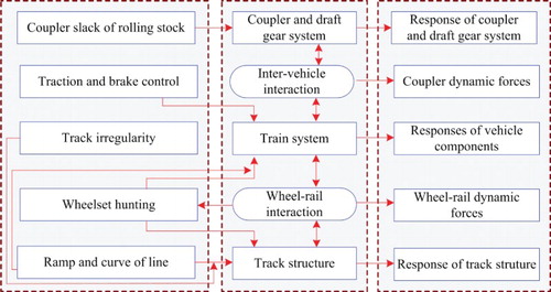
Besides, affected by the train running speed and track geometries, the wheel–rail dynamic forces excited by the track irregularities have an influence on the train–track coupled system in a wide frequency range.[50] Simultaneously, the working status of coupler and draft gear system will also be changed, thus resulting in the different interactions between the adjacent vehicles. Therefore, the coupler and draft gear subsystem, the train and the track subsystems are interrelated.

3. Modular modelling method of heavy-haul train–track coupled system

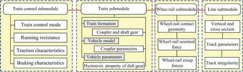
Considering the structure forms and application practices of the modern heavy-haul train and track, the heavy-haul train–track interaction model is developed based on the vehicle–track coupled dynamics.[36,50] And the modular method is applied (see Figure 2). The whole system mainly contains four parts: the train control submodule, the train submodule, the wheel–rail relation submodule, and the line submodule. The wheel–rail relation integrates the train subsystem and the track subsystem as a coupled system. The train control module provides the operation control functions for the whole train–track system, which also determines the train operation status in the different line conditions.

Figure 2. Modularised modelling of 3-D heavy-haul train–track coupled dynamics model.

4. 3-D heavy-haul train–track coupled model

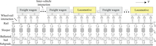
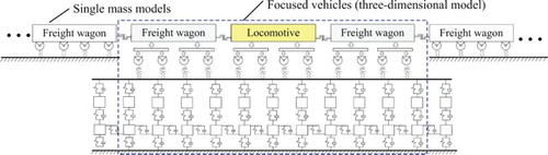
Based on the basic principle of the train–track interactions and modelling method given above, the heavy-haul train–track coupled dynamic model is established. In order to simulate the dynamic behaviours of the train and the track, their structure characteristics need to be recognised firstly. The basic components of a certain type vehicle are definite. For example, a locomotive generally consists of the carbody, bogie frames, traction motors and wheelsets, while a freight wagon is usually composed by the carbody, side frames, bolsters and wheelsets. For the ballasted track structure which is most widely used in the heavy-haul railways, it also has the normative form. Figure 3 shows the schematic diagram of the typical heavy-haul train–track coupled dynamic model, in which the locomotives are distributed in different positions of the train (Distributed Power mode), and the track is the commonly used ballasted track.

Figure 3. Heavy-haul train–track coupled dynamic model (side view).

The relevant dynamic models of the locomotive, the freight wagon and the ballasted track could be found in some literatures.[34–36] Specially, the forces such as the traction force, the braking force, the coupler forces and the running resistance should be also considered in the vehicle model. Furthermore, the possible large creepage between the wheel and the rail needs to be taken into account. Their detailed calculation methods are given as follows.

4.1. Calculation of wheel–rail forces

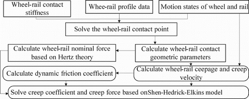
Under the train driving or braking conditions, the larger creepage may happen in the wheel–rail contact surface. To calculate the wheel–rail forces accurately in these cases, Knothe et al. [51] pointed out that the variable relationship between the wheel–rail tangential force and the creepage can be depicted by introducing the dynamic wheel–rail friction coefficient into the Vermeulen–Johnson model or the Shen–Hedrick–Elkins model. In this article, the same method is also adopted. Figure 4 shows the general calculation flow chart of the wheel–rail forces.

Figure 4. Calculation flowchart of wheel–rail forces.

In order to reflect the large creep speed and consider the effect of the rail vibrations, the creepage calculation formulas are given as, (1) where the symbols V₁, V₂ and Ω₃ are the instantaneous running speed, lateral speed and spin speed at the wheel mass centre, respectively; V_r1, V_r2 and Ω_r3 successively denote the peripheral speed, lateral speed and spin speed at the wheel contact point; and V_Ry represents the lateral speed induced by the rail vibration and track irregularity variation.

With the creep speed increasing, the wheel–rail friction coefficient has a descending trend. According to the field test results of the wheel–rail friction coefficient in the braking condition, the empirical formula of the variable friction coefficient is expressed as [52] (2) where, f_stat and f_kin represent the static and dynamic friction coefficients, respectively; v_s denotes the wheel–rail creep velocity; and f_stat is set to be 0.45 and 0.25 for the dry and the wet rail surface conditions, respectively. Then the wheel–rail creep forces are calculated by introducing the variable friction coefficient into the Shen–Hedrick–Elkins model.[53]

4.2. Calculations of train driving and braking forces

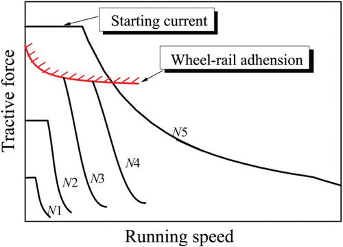
The train tractive force is an external force which can be adjusted as required. It is calculated from the perspective of the driver’s operation. For the locomotive with the property of step speed regulation, its traction characteristics can be described as a number of traction force curves related to the driver controlling handle positions, as shown in Figure 5. The different traction forces can be obtained by changing the handle positions. With the current running speed v of the locomotive and the handle position N, the traction force can be calculated by interpolating in the traction force curves. However, during the startup process, the maximum driving force is limited by the starting current and wheel–rail adhesions. As for the locomotive with the feature of stepless speed regulation, the traction force is dependent on the running speed and the given percentage, which can be calculated in formula (3). (3) where, f(v) denotes the maximum traction force, n% is the percentage of control.

Figure 5. Traction characteristic curves of a locomotive.

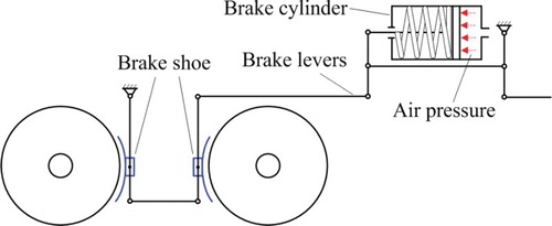
For the calculation of the braking forces, the difference of the brake modes should be considered. At present, the brake shoe braking and electric braking are the two main types used in the heavy-haul train. The force source for the brake shoe braking is from the compressed air (see Figure 6), which distributes in both the locomotives and the freight wagons. As the pneumatic bake is applied, the braking force can be expressed as the product of the brake shoe pressure and the friction coefficient of the contact interface. The brake shoe pressure K is calculated as [54] (4) where d_z is the diameter of the brake cylinder (unit: mm); p_z is the air pressure in the brake cylinder (unit: kPa); η_z is the computational transmission efficiency of foundation brake gear; γ_z is the braking leverage; and n_z and n_k are the numbers of cylinder and brake shoes, respectively. For the air pressures in the brake cylinders of the wagons and the locomotives, they can be obtained from the train pneumatic braking test. And the friction coefficient of brake shoe can be obtained from the experiments or the relevant railway occupation standards.

Figure 6. Brake shoe system.

As for the electric braking which is only applied in the locomotive, it can be regarded as the inverse process of the traction. The braking force is limited by the motor power and the wheel–rail adhesion. In the case of the step speed regulation, the electric braking force can be calculated by interpolating in the electric braking force curves according to the running speed and braking handle position. If the locomotive has the property of stepless speed regulation, the braking force is dependent on the running speed and the given percentage.

4.3. Dynamic model of coupler and draft gear system

For the heavy-haul locomotives and freight wagons in China, the non-rigid automatic couplers with the self-centring ability are commonly used. There is usually a free clearance between the two connected couplers, which permits them to move relatively in the vertical direction. And in the horizontal direction, the coupler can sway within a small angle relative to its draft key.

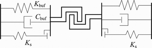
In the train longitudinal dynamics, a pair of connected couplers is usually considered as an entirety without mass. The typical simplified mathematic model [55] is shown in Figure 7. The symbols K_buf and C_buf are the stiffness and the damping of the draft gear, respectively. And K_s denotes the structural stiffness of carbody. However, K_buf and C_buf are not two constants, but have the nonlinear characteristics. For the convenient simulation, the stiffness and damping of the draft gear are usually described by the hysteresis curves. Being different from the train longitudinal dynamic model, the inter-vehicle interactions in the 3-D train model will be affected comprehensively by the coupler forces in the longitudinal, lateral and vertical directions. Therefore, for the typical coupler and draft gear package used in China, the corresponding calculation methods are given below.

Figure 7. Dynamic model of heavy-haul coupler and draft gear system.

(1) Coupler longitudinal force between vehicles

The hysteresis characteristics of the draft gear are represented as the misaligned loading and unloading curves, as shown in Figure 8.

Figure 8. Hysterisis characteristics of the draft gear.

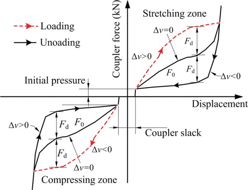
The loading or unloading working status in the draft gear is usually determined by both the relative displacement and speed between the adjacent vehicles. There exists a jump for the coupler force when the draft gear switches between the loading and unloading conditions, which means that the force variation in the draft gear is discontinuous. The problem of discontinuity point should be solved to guarantee the continuity of the differential equations and the dynamical balance of the system. The handling method of the dry friction damping is used. The formula for the calculation of the coupler longitudinal force is given as, (5) where F_cx is the coupler longitudinal force; v_f is the switching speed between the loading and unloading conditions; and F₀ and F_d represent the spring force and damping force of the coupler and draft gear system, respectively.

(2) Coupler lateral force

The coupler lateral force includes two parts, namely, the lateral component of the coupler force and the lateral force induced by the coupler restoring moment. The values of these two forces are related to the magnitude of the coupler swing angle in the horizontal plane. Besides, the typical couplers widely used in China usually have the self-centring abilities. In the simulation, it is assumed that the connected two couplers are regarded as a rigid-straight bar without the relative rotations. The swing angle of the coupler relative to the car body is defined as positive when it rotates around its draft key clockwise in the top view, otherwise it is negative.

When the train negotiates a curved track, the coupler swing angle will be affected by the line alignment. The coordinates of the track centre line are shown in Figure 9. For the ith vehicle, the positions of the front and rear centre pins are determined by the coordinates (x_ti1, y_ti1) and (x_ti2, y_ti2), respectively. Then, the coordinate values of the carbody mass centre are obtained as (6)

Figure 9. Geometric relationship between the couplers and the vehicles in a curved track.

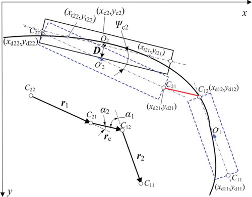
When the centre line of the draft keys in the carbody has the displacement D and the yaw angle ψ_c, the coordinates of the front and rear draft keys in the absolute coordinate system are expressed as (7) where . L equals l_cg and −l_cg for the front and rear draft keys, respectively. The coordinates of the draft keys C₁₁, C₁₂, C₂₁ and C₂₂ of the adjacent two vehicles can be finally calculated by formula (7). Connecting these four points, three two-dimensional vectors r₁, r₂ and r_c are obtained. Then the intersection angles of these vectors can be obtained conveniently. The swing angles of the couplers relative to the centre lines of the front and the rear vehicles are calculated, respectively, in formula (8). (8) where k(r) is the corresponding gradient of the vector r in the global reference system.

Actually, the coupler swing angle cannot increase continuously, and its amplitude is limited by the structures of the coupler and the draft gear system. Once the coupler angle exceeds the free swing limit (δ_y), a restoring torque will generate against its swing motion. The restoring torques can be classified into two main forms according to their action principles (see Figure 10(a)). One is called the rigid stop characteristic, which means the restoring torque changes linearly with the variation of the swing angle. The other one is called the nonlinear impedance characteristic, which indicates that the value of the restoring torque depends on the compression amount and load of the draft gear. More specifically, when the coupler swing angle exceeds the free limit value in this case, the coupler needs to firstly overcome the resistance torque caused by the initial pressure of the draft gear, and then it can compress the draft gear.

Figure 10. Calculation of coupler lateral force: (a) coupler restoring torque, (b) coupler force analysis.

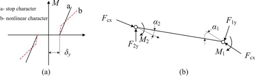
The coupler lateral forces acting on the draft keys can be calculated according to the force equilibrium conditions (see Figure 10(b)). (9) where L_cp is the length of the two coupling couplers, and M₁ and M₂ represent the coupler restoring moments.

(3) Coupler vertical force

The coupler vertical force is mainly composed of the friction force occurring in the coupler contact interface. Referring to Garg and Dukkipati,[55] the calculation model of the coupler vertical force can be simplified as a nonlinear spring-friction element with the coupler clearance. Figure 11 shows the schematic diagram of the calculation model of the coupler vertical force. The dynamic responses of the vehicle system are the main reasons that induce the vertical motion of the coupler head. And the vertical and pitching motions of the carbody have the primary influence.

Figure 11. Calculation model of coupler vertical force.

The relative displacement and speed between the adjacent vehicles in the vertical direction are calculated as (10) When the longitudinal relative displacement is smaller than the coupler slack δ_fc, the friction force in the vertical direction is F_cz = 0. Otherwise, two different cases need to be clarified as follows.

(1) If , then (11)

(2) If , then (12) where v_r is the switching speed, and μ₀ and μ_d are the static and dynamic friction coefficients, respectively.

4.4. Mathematical model of cross and vertical section in railway line

From the aspect of the geometry, the railway line can be regarded as the combinations of the vertical section and cross sections. These two type sections have different effects on the train dynamic behaviours.

(1) Vertical section model of railway line

Lots of researches have shown that, the line gradient i% is the key factor affecting the train longitudinal impulse. The mathematical description of the vertical section variation can be simplified as the changing gradient i% along the line length l, that is i% = f(l) .

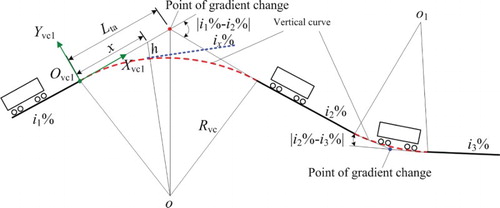
However, the issue concerning whether the vertical curve should be considered in the vertical section model needs to be further clarified. At the point of gradient change in the actual line, the vertical curve is inserted to connect the two slopes when the gradient difference of the adjacent slopes exceeds a threshold value. In the previous model of the vertical section, the influence of the vertical curve is usually neglected. In general, the vertical curve cannot significantly change the influence extent of the slope gradient difference on the train longitudinal impulse, but it can affect the distributions of the coupler longitudinal forces. Therefore, the vertical curve is considered in this article.

Figure 12 shows the geometric relationship between the slope and the vertical curve with radius R_vc. The tangent line length of the vertical curve is ,[56] and the length of the vertical curve is . Then, the gradient in the vertical curve can be expressed as, (13) where, the top and bottom signs of ± are selected for the convex and concave vertical curves, respectively.

Figure 12. Geometric relation between slope and vertical curve.

(2) Cross section model of railway line

The basic elements of the railway plane line mainly include the straight lines, the transition curves and the circular curves. In a curved track, both the superelevation and the track curvature will directly influence the vehicle running behaviours. Furthermore, the plane coordinates of the railway line affect the relative positions of the adjacent vehicles significantly, which may have a great effect on the inter-vehicle lateral interaction. Considering the above factors comprehensively, it is necessary to establish the cross section model in detail.

For the plane curve with the radius of R, both the lengths of the entry and exit transition curves are assumed to be l_h, and the deflection angles of the transition curve and circular curve are defined as θ_tc = l_h/(2R) and θ_cc, respectively. Their local coordinate systems are shown in Figure 13(a). OXY represents the global coordinate system of the plane curve, O_tc1X_tc1Y_tc1, O_ccX_ccY_cc and O_tc2X_tc2Y_tc2 denote the local coordinate systems of the entry transition curve, the circular curve and the exit transition curve in sequence.

Figure 13. Cross section geometries: (a) coordinate; (b) coordinate transform of exit transition curve.

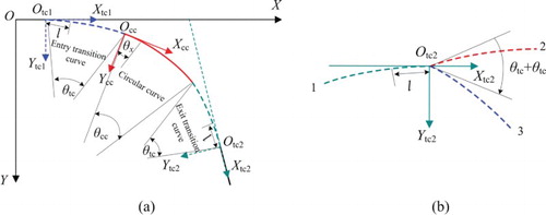
Considering that the transition curve commonly used in China is the spiral line, the coordinates of the entry transition curve in the global coordinate system OXY can be expressed as (14) where x_se is the coordinate increment of the straight line. In the reference system O_ccX_ccY_cc, the coordinates of each point in the circular curve are calculated by (15)

Then, the coordinates of the circular curve in the global coordinate system can be obtained as (16) where (x_tce, y_tce) are the coordinates of the end point of the entry transition curve.

For the coordinate calculation of the exit transition curve, the effects of the entry transition curve and circular curve should be considered comprehensively. As Figure 13(b) shows, the exit transition curve needs to be moved to position 2 from position 1 firstly, and then it is rotated to position 3 according to the deflection angles of the entry transition curve and the circular curve, and finally it is moved and connected to the end of the circular curve.

The coordinate values for the other track sections can also be calculated according to the steps described above. Besides, the superelevation of the outer rail, the curve curvature and other parameters can be obtained from the cross section. Particularly in the transition curve, the commonly used form of outer rail superelevation is the linear run-off elevation, and its curvature and the superelevation meet the linear relationship.

5. Solving method of train–track coupled dynamic model

In the train–track coupled dynamic model, there exist a huge number of DOFs. To achieve the fast solution on the dynamic responses of this large-scale system, the Zhai method [57] is used to numerically integrate the differential equations. However, it is still quite time-consuming if each vehicle is regarded as a 3-D model and the track elasticity is also considered simultaneously, as shown in Figure 3. It is challenging for a common computer to accomplish the massive calculations. Therefore, an efficient solving technique is necessary to be developed on the premise of satisfying the precision requirements. For increasing the solving speed, the dynamic model can be simplified to a certain degree according to the analysis purpose. If the train longitudinal dynamics is more concerned, each vehicle can be simplified as the single-mass model. If the dynamic performance of the vehicle subjected to the coupler force is focused, the focused vehicles can be modelled in detail while others are simulated by the mass block. On account of this, the solving methods are given.

5.1. Solving methods

For the long train–track coupled system, the solving flow is illustrated in Figure 14. The basic processes are given as follows:

1. Carry out the analysis of the train longitudinal dynamics, and every vehicle is simplified as the one-dimensional mass point.

2. Obtain the distributions of the coupler longitudinal forces in the whole train, then find out the occurring position of the largest coupler force. And the vehicles near the maximum coupler force are of being focused thoroughly.

3. Convert the single-mass models of vehicles near the largest coupler force to the 3-D vehicle–track coupled models (see Figure 15).

4. Recalculate the train dynamic response of the mixed model, and comprehensively evaluate the indices of the wheel–rail forces, derailment coefficient, track displacements, coupler swing angle, and so on.

Figure 14. Flow chart for calculation of train–track coupled dynamic model.

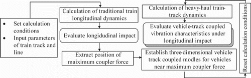
Figure 15. Mixed dynamic model of a heavy-haul train.

By applying the above methods, the computation efforts for solving the large system can be reduced. And the analysis requirements can also be satisfied.

An important issue for the accurate calculation using the developed mixed dynamic model is to determine the number N of the 3-D vehicle models in the concerned position of the train. When the train negotiates a curved track or runs on the track irregularities, there are the longitudinal, lateral and vertical dynamic forces between the adjacent two vehicles. However, the spatial motions of the 3-D vehicles will be constrained by the vehicles modelled as the one-dimensional single mass. Therefore, an inevitable problem needs to be answered. That is, for the concerned position, how many vehicles represented by the 3-D model are required to reduce the negative effects of the single-mass models on the dynamic responses of the focused vehicles.

In order to clarify this question, the simulation experiments for two short trains with the freight wagon marshalling mode and the locomotive-wagon marshalling mode are carried out to determine the minimum value of the number N required.

5.2. Determination of the required number of the freight wagons modelled as 3-D model

The short train is only composed of the freight wagons, as shown in Figure 16. The vehicles at both the train ends are modelled as the single-mass model, while other wagons are modelled as the 3-D model. The middle wagon is selected as the research object. The last vehicle runs at a constant speed, while the braking force F_B is exerted on the vehicles before the focused wagon to generate a target coupler force in the position A. Hereby, the wheel–rail dynamic responses of the middle wagon under the action of coupler force can be calculated.

Figure 16. Short train model composed only by freight wagons.

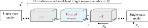
In the dynamic model, the lateral dynamic behaviours of the train are analysed by applying a target coupler force of 2200 kN. The type of heavy-haul wagon is C80, and the train running speed is 80 km/h. According to the distributions of the sharp curves in Daqin and Shuohuang heavy-haul railway lines in China, the curve radius, outer rail superelevation and the transition curve length are selected as 400 m, 100 mm and 80 m, respectively.

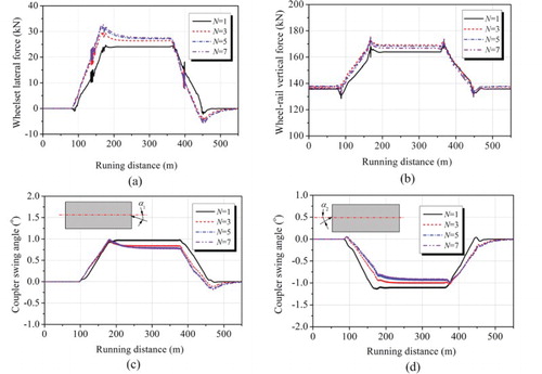
The dynamics indices of the focused freight wagon are extracted to illustrate the effect of the number of the vehicles represented by the 3-D model, as shown in Figure 17. It can be seen that, if only the focused wagon is modelled in detail, namely N = 1, the constraint effect from the adjacent vehicles represented by the single-mass models can be clearly identified, and a huge discrepancy is generated between the results of this case and that of other cases where N equals to 3, 5, and 7. However, as the number N exceeds 3, the curves of the same index for the different N are very close with each other. Therefore, while one freight wagon in a train is focused in the analysis, treating this wagon and its adjacent two wagons as the 3-D models are enough to eliminate the constraint effects of the one-dimensional models in other positions.

Figure 17. Dynamic performance of the focused vehicle with different number of 3-D wagon models: (a) wheelset lateral force of axle1; (b) wheel–rail vertical force of outer wheel in axle1; (c) swing angle of front coupler; (d) swing angle of rear coupler.

5.3. Determination of the required number of the wagons modelled as 3-D model near focused locomotive

In the combined train, the locomotives usually distribute in the head, the end and the middle positions. For the sake of improving the ride quality, the horizontal suspension stiffness in the locomotive is much smaller than that in the wagon. This means the dynamic behaviours of the locomotive may be more sensitive to the coupler force. For these reasons, once the focused vehicle in the heavy-haul train is a locomotive, all of the centralised locomotives in this position should be considered as the 3-D models.

Then the key question occurs that whether it is necessary to use the 3-D models to simulate the neighbouring freight wagons of the locomotives. In this investigation, the heavy-haul locomotive HXD₂ and freight wagon C80 which are widely used in China are employed. The basic analysis method, curve parameters and the train running speed are the same as that employed in Section 5.2. Figure 18 displays the dynamic model of the marshalling train used in this subsection. It is assumed that there are two HXD₂ locomotives locating in the middle of the train, and the simulated results are extracted from the second locomotive which is viewed as the focused vehicle to demonstrate the effect of the number of the 3-D wagons.

Figure 18. Dynamic model of a train composed by locomotives and freight wagons.

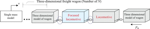
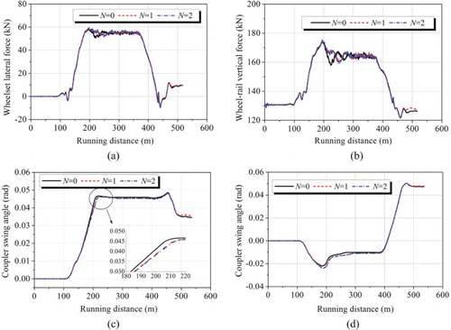
Figure 19 shows the calculated results of the dynamic responses of the focused locomotive with different number of the 3-D wagons. It is indicated that the number N has a slight effect on the wheel–rail forces and the coupler dynamic behaviours. When the number N varies between 1 and 3, the responses of a certain index vary with the same trend. Especially, when N equals to 1 and 2, the time histories of the same index almost overlap with each other. It is indicated that a high calculation accuracy can be obtained when one or more freight wagons connected to the locomotive are considered as the 3-D model.

Figure 19. Dynamic performance of the focused locomotive with different number of 3-D wagon models: (a) wheelset lateral force of axle1; (b) wheel–rail vertical force of outer wheel in axle1; (c) swing angle of front coupler; (d) swing angle of rear coupler.

When the vehicle is subjected to the coupler pulling force or the focused vehicles locate at the train ends, the corresponding dynamics indices are also analysed which are not shown in this article. It can be also concluded that the dynamic performance of the focused vehicle could be reflected as well by using the aforementioned methods.

In summary, the principle of using the 3-D model for the dynamic analysis of a heavy-haul train can be summarised as: (1) if the maximum coupler force occurs in the freight wagon which is far away from the locomotives, at least three wagons around the maximum coupler force should be modelled as the 3-D models; (2) if the maximum coupler force appears in the locomotives, the centralised distributing locomotives and their adjacent two freight wagons in this area ought to be simulated simultaneously by the 3-D models.

6. Experimental verification

In this section, the wheel–rail dynamic interaction and the interaction between vehicles are validated by comparing the calculated results with that from the field test. The verification in several conditions are given below.

6.1. Verification by coupler longitudinal force of a combined train under braking conditions

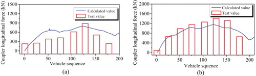
The running test results of a 20,000 t heavy-haul combined train under the braking conditions in ref. [58] are employed in this subsection for verification. The test was carried out on Daqin heavy-haul railway in 2004. The train consisted of the locomotive SS4 and the freight wagon C80 with the formation of SS4 + 51 × C80 + SS4 + 51 × C80 + SS4 + 51 × C80 + SS4 + 51 × C80. The field tests in the full service and emergency braking conditions were conducted on a track section with the −12‰ slope gradient. The initial speed at the brake application was 75 km/h.

Figure 20 shows the maximum coupler forces along the train in the different operation modes. It is clear that the basic varying trend of the calculated results broadly coincides with that of the test results. The difference of their maximum coupler forces is below 10%. Similarly, for the full service braking condition, the coupler force distributions calculated are also generally consistent with the test results.

Figure 20. Coupler longitudinal forces of 20,000 t combined train in braking conditions: (a) emergency braking; (b) full service braking.

6.2. Verification of train dynamic characteristics under electric braking condition

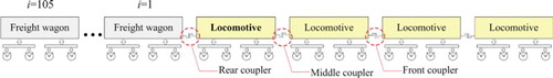
To examine the dynamic responses of the coupler and the locomotive in the braking condition, the test data of a 10,000 t train obtained from the literature [59] is used. In June 2008, Taiyuan railway administration organised the running safety test of a 10,000 t heavy-haul train, and the test was carried out in the straight sections of North Tongpu railway and Daqin railway. The test purpose was to confirm the working stability of the coupler and the draft gear system when they were subjected to a large coupler compression force. By exerting the electric braking in the different levels, the compression force of the coupler system increased gradually. The train formation was shown in Figure 21, and the focused couplers were the front, the middle and the rear couplers. The instrumented wheelset was the third wheelset of the 3rd locomotive.

Figure 21. Formation of a 10,000 t heavy-haul train.

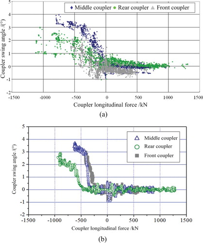
Comparisons between the test results and simulation results of the coupler swing angles under the electric braking condition are made and shown in Figure 22. It can be seen in Figure 22(a) that the couplers sway near the centring position under the coupler pulling force, and the swing amplitudes decrease with the increase of the pulling force. Conversely, the coupler will tilt to one side as the coupler compressing force enlarges to a certain degree. The phenomenon can be explained as that, in the electric braking condition, the locomotives almost brake at the same time, and the latter coupler will bear a larger longitudinal coupler force due to the inertia effect of rear wagons. Besides, all of the locomotive couplers have the same coupler-stabilising abilities. Consequently, the coupler subjected to the larger compressing force will swing more obviously. Specifically, for the front and the middle couplers, the latter one bears a larger coupler force, so the angle of middle coupler is larger than that of the front coupler. But, for the rear coupler, it is connected with the wagon coupler which has a stronger coupler-stabilising ability. For this situation, even if there is the largest coupler force acting on the rear coupler, its tilt angle magnitude is smaller than that of the middle coupler. For the three focused couplers, the middle coupler has the largest swing angle of 4°, and the rear coupler swing angle is less than 3°. The calculation results in Figure 22(b) indicate that the variations of the coupler swing angles follow the similar trend as that displayed in Figure 22(a). It can be found that the swing angles of the middle and the rear couplers are slightly below 4° and 3°, respectively. Overall, the corresponding coupler angles in Figure 22 change following the same rules, and the calculated and tested results coincide well with each other.

Figure 22. Comparisons of tested and calculated coupler swing angles: (a) tested results; (b) calculated results.

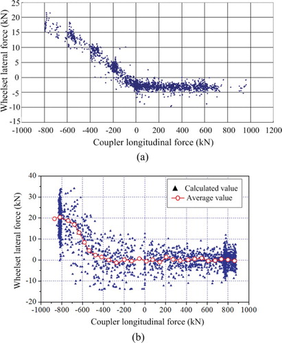
The wheelset lateral forces obtained from the field test and the simulation are compared and displayed in Figure 23. The results reveal that the wheelset lateral forces present statistically the unidirectional increase when the compressing coupler force increases. The test wheelset force is slightly lower than the calculated values, which is most likely caused by the differences of the data processing method and the track irregularities. It is worth pointing out that the test data are closed to the average values of the calculated results.

Figure 23. Wheelset lateral force of locomotive under electric braking condition: (a) tested results; (b) calculated results.

6.3. Verification through heavy-haul train curving performance

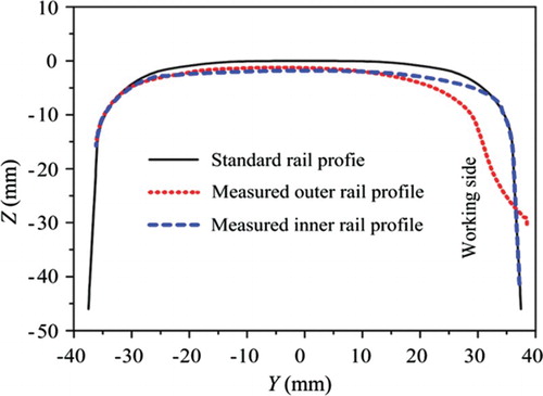
For the validation of the wheel–rail dynamic interactions of the heavy-haul train on curve, the curving performance of the train composed of the C70 freight wagons is analysed. The calculated results are compared with the tested results extracted from the literature.[60] The curve has a 500 m radius. Due to the wheel–rail wear, the actual profiles of the outer and the inner rails present the asymmetries, as shown in Figure 24. To reflect the actual track states, the measured rail profiles are also used in the simulation. The train runs at a constant speed of 60 km/h.

Figure 24. Measured rail profiles in curved track.

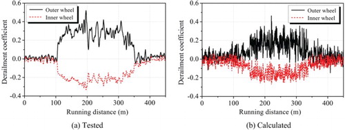
Comparisons between the simulated and tested results of the wheel–rail lateral force, the wheel–rail vertical force and the derailment coefficient are displayed in Figures 25–27. It is illustrated that the varying rule of each simulated dynamic index agrees well with that of the tested result. The tested maximum values of the outer wheel–rail lateral force, the wheel–rail vertical force and the derailment coefficient are 65 kN, 127 kN and 0.52, respectively. Correspondingly, the calculated peak values of these indices are 59 kN, 142 kN and 0.48 in sequence, which are close to the tested values. For the inner wheel–rail dynamic indices, the tested amplitudes of the wheel–rail lateral force, the wheel–rail vertical force and the derailment coefficient are 34 kN, 133 kN and 0.33, respectively, while the simulated values are 32 kN, 133 kN and 0.29, successively.

Figure 25. Comparisons of wheel–rail lateral forces between (a) tested results and (b) calculated results.

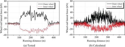
Figure 26. Comparisons of wheel–rail vertical forces between (a) tested results and (b) calculated forces.

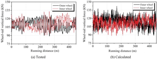
Figure 27. Comparisons of derailment coefficients between (a) tested results and (b) calculated results.

In summary, the reliability of the heavy-haul train–track coupled dynamics model is supported by the consistence between the calculated and tested results. It can be used in the analysis and evaluation of the dynamic interactions between the long heavy-haul train and track.

7. Conclusions

The effects of the train longitudinal coupler force on the locomotive wheel–rail dynamic interactions are obvious once the couplers tilt laterally. The train running safety and the track service performance are still the essential challenging problems in some severe cases. In this paper, aiming at the typical heavy-haul train and track system in China, a train–track coupled dynamics model of a long heavy-haul train and ballasted track has been established. At the positions where the most violent longitudinal impulse appears, the dynamic performances of the locomotives or the freight wagons are of great concerned. Meanwhile, a solving method has been developed to calculate the dynamic response of the large-scale system. The dynamic model is verified through comparisons between the simulated and the tested results with respect to the train longitudinal impulse, the wheel–rail dynamic interactions under the braking conditions, and the curving performance of heavy-haul trains. Admittedly, the heavy-haul train and track system integrate various factors, and more comprehensive investigations on the numerical model should be carried out in the future work.

Disclosure statement

No potential conflict of interest was reported by the authors.

Additional information

Funding

This research was supported by National Natural Science Foundation of China [Grant No. 51478399], the Scientific Discipline Development Project of Southwest Jiaotong University (2012), and by the Science and technology research project of Hebei Province [BJ2016047].

References

- Martin GC, Hay WW. Method of analysis for determining the coupler forces and longitudinal motion of a long freight train in over-the-road operation. Report, Illinois, America; 1967.
- Martin GC, Tidman H. Detailed longitudinal train action model. Report No R-221, Chicago, America; 1977.
- Genin J, Ginsbergand JH, Ting EC. Longitudinal track-train dynamics: a new approach. J Dyn Syst Meas Control. 1974;12:466–469. doi: 10.1115/1.3426847
- Duncan IB, Webb PA. The longitudinal behavior of heavy haul trains using remote locomotives. In: Proceedings of Fourth International Heavy Haul Conference. Brisbane; 1989. p. 587–590.
- Jolly BJ, Sismey BG. Doubling the length of coals trains in the Hunter Valley. In: Proceedings of Fourth International Heavy Haul Conference. Brisbane; 1989. p. 579–583.
- Van Der Meulen RD. Development of train handling techniques for 200 car trains on the Ermelo-Richards Bay line. In: Proceedings of Fourth International Heavy Haul Conference. Brisbane; 1989. p. 574–578.
- Cole C. Longitudinal train dynamics. In: Iwnicki S, editors. Handbook of railway vehicle dynamics. London: Taylor& Francis; 2006. p. 239–278.
- Bowey R. Research on longitudinal train dynamics in Australia. In: Proceedings of 7th Heavy Haul Conference. Brisbane; 2001. p. 225–230.
- Cole C. Improvements to Wagon connection modelling for longitudinal train simulation. In: Proceedings of Conference on Railway Engineering. Rockhampton; 1998. p. 187–194.
- Scown B, Roach D, Wilson P. Freight train driving strategies developed for undulating track through train dynamics research. In: Proceedings of Conference on Railway Engineering. Adelaide; 2002. p. 329–336.
- Simson S, Cole C, Wilson P. Evaluation and training of drivers during normal train operations. In: Proceedings of Conference on Railway Engineering. Wollongong; 2000. p. 1–17.
- Chou M, Xia X, Kayser C. Modelling and model validation of heavy-haul trains equipped with electronically controlled pneumatic brake systems. Control Eng Pract. 2007;15:501–509. doi: 10.1016/j.conengprac.2006.09.006
- Diana G, Cheli F, Belforte P, Melzi S. Numerical and experimental investigation of heavy freight train dynamics. In: Proceedings of IMECE 2007. Washington; 2007. p. 1–10.
- Cole C, Sun YQ. Simulated comparisons of wagon coupler systems in heavy haul trains. Proc Inst Mech Eng F, J Rail Rapid Transit. 2006;220:247–256. doi: 10.1243/09544097JRRT35
- Shabana AA, Aboubakr AK, Ding L. Development of a new train coupler model using non-inertial coordinates. Report. Chicago; 2010.
- Massa A, Stronati L, Aboubakr AK, Shabana AA, Bosso N. Numerical study of the non-inertial systems: application to train coupler systems. Nonlinear Dyn. 2012;68:215–233. doi: 10.1007/s11071-011-0220-2
- Ansari M, Esmailzadeh E, Younesian D. Longitudinal dynamics of freight trains. Int J Heavy Veh Syst. 2009;16(1/2):102–131. doi: 10.1504/IJHVS.2009.023857
- Nasr A, Mohammadi S. The effects of train brake delay time on in-train forces. Proc Inst Mech Eng F, J Rail Rapid Transit. 2010;224:523–534. doi: 10.1243/09544097JRRT306
- Specchia S, Afshari A, Shabana AA, Caldwell N. A train air brake force model: locomotive automatic brake valve and brake pipe flow formulations. Proc Inst Mech Eng F, J Rail Rapid Transit. 2013;227(1):19–37. doi: 10.1177/0954409712447230
- Afshari A, Specchia S, Shabana AA, Caldwell N. A train air brake force model: car control unit and numerical results. Proc IMech E, Part F, J. Rail Rapid Transit. 2013;227(1):38–55. doi: 10.1177/0954409712447231
- Thomas RL, MacMillan RD, Martin GC. Quasi-static lateral train stability model-technical manual. Report. Chicago; 1976.
- Raidt JB, Shum KL, Martin GC, Garg VK. Detailed vertical train stability model-technical documentation. Report. Chicago; 1977.
- Durali M, Jalili MM. Time saving simulation of long train derailment. In: Proceedings of IMECE2008. Boston; 2008. p. 461–465.
- Wagner S. Derailment risk assessment [Master thesis]. Rockhampton, Australia: Central Queensland University; 2004.
- Jeong DY, Lyons ML, Orringer O, Perlman AB. Equations of motion for train derailment dynamics. In: Proceedings of the 2007 ASME Rail Transportation Division Fall Technical Conference. Chicago; September; 2007. p. 21–27.
- Simon SA. Three axle locomotive bogie steering, simulation of powered curving performance passive and active steering bogies [Ph.D thesis]. Queensland, Australia: Central Queensland University; 2009.
- Xu ZQ, Ma WH, Wu Q, Luo SH. Coupler rotation behaviour and its effect on heavy haul trains. Veh Syst Dyn. 2013;51(12):1818–1838. doi: 10.1080/00423114.2013.834369
- Xu ZQ. Research on adaptability of coupler systems on 33t axle load heavy haul locomotive [Ph.D thesis]. Chengdu, China: Southwest Jiaotong University; 2013.
- Belforte P, Cheli F, Diana G, Melzi S. Numerical and experimental approach for the evaluation of severe longitudinal dynamics of heavy freight trains. Veh Syst Dyn. 2008;46(Suppl.):937–955. doi: 10.1080/00423110802037180
- Pugi L, Rindi A, Ercole AG, et al. Preliminary studies concerning the application of different braking arrangements on Italian freight trains. Veh Syst Dyn. 2011;49(8):1339–1365. doi: 10.1080/00423114.2010.505291
- Cole C, McClanachan M, Spiryagin M, Sun YQ. Wagon instability in long trains. Veh Syst Dyn. 2012;50(Suppl.):303–317. doi: 10.1080/00423114.2012.659742
- Zhang WH, Chi MR, Zeng J. A new simulation method for the train dynamics. In: Proceedings of 8th International Heavy Haul Conference. Rio de Janeiro; 2005. p. 773–778.
- Chi MR, Zhang WH, Zeng J. A study on train dynamics behavior by suing a new simulation method. In: Proceedings of 19th IAVSD Symposium. Milan; August, 2005.
- Zhai WM, Sun X. A detailed model for investigation vertical interaction between railway vehicle and track. Veh Syst Dyn. 1994;23(Suppl.):603–615. doi: 10.1080/00423119308969544
- Zhai WM, Cai CB, Guo SZ. Coupling model of vertical and lateral vehicle/track interactions. Veh Syst Dyn. 1996;26(1):61–79. doi: 10.1080/00423119608969302
- Zhai WM. Vehicle–track coupled dynamics. 4th ed. Beijing: Science Press [in Chinese]; 2015.
- Zhai W, Gao J, Liu P, Wang K. Reducing rail side wear on heavy-haul railway curves based on wheel–rail dynamic interaction. Veh Syst Dyn. 2014;52(Suppl.):440–454. doi: 10.1080/00423114.2014.906633
- Fröhling RD. Low frequency dynamic vehicle/track interaction: modeling and simulation. Veh Syst Dyn. 1998;28(Suppl.):30–46. doi: 10.1080/00423119808969550
- Oscarsson J, Dahlberg T. Dynamic train/track/ballast interaction: modelling and simulation. Veh Syst Dyn. 1998;28(Suppl.):73–84. doi: 10.1080/00423119808969553
- Auersch L. Vehicle–track–interaction and solid dynamics. Veh Syst Dyn. 1998;28(Suppl.):553–558. doi: 10.1080/00423119808969586
- Hou K, Kalousek J, Dong R. A dynamic model for an asymmetrical vehicle/track system. J Sound Vib. 2003;267:591–604. doi: 10.1016/S0022-460X(03)00726-0
- Nielsen JCO, Oscarsson J. Simulation of dynamic train–track interaction with state-dependent track properties. J Sound Vib. 2004;275:515–532. doi: 10.1016/j.jsv.2003.06.033
- Baeza L, Roda A, Carballeira J, Giner E. Railway train–track dynamics for wheelflats with improved contact models. Nonlinear Dyn. 2006;45:385–397. doi: 10.1007/s11071-005-9014-8
- Chaar N. Wheelset structural flexibility and track flexibility in vehicle–track dynamic interaction [PhD thesis]. Stockholm: Royal Institute of Technology (KTH); 2007.
- Sun YQ, Simson S. Nonlinear three-dimensional wagon-track model for the investigation of rail corrugation initiation on curved track. Veh Syst Dyn. 2007;45(2):113–132. doi: 10.1080/00423110600863407
- Sun YQ, Simson S. Wagon-track modeling and parametric study on rail corrugation initiation due to wheel stick-slip process on curved track. Wear. 2008;265:1193–1201. doi: 10.1016/j.wear.2008.02.043
- Johansson A, Nielsen JCO, Bolmsvik R, Karlström A, Lundén R. Under sleeper pads-influence on dynamic train–track interaction. Wear. 2008;265:1479–1487. doi: 10.1016/j.wear.2008.02.032
- Oyarzabal O, Gómez J, Santamarĺa J, Vadillo EG. Dynamic optimization of track components to minimize rail corrugation. J Sound Vib. 2009;319(3–5):904–917. doi: 10.1016/j.jsv.2008.06.020
- O’Brien EJ, Taheri A, Gavin K. The influence of subgrade subsidence on train track dynamic interaction. Civil-Comp, In: Proceedings of the First International Conference on Railway Technology: Research, Development and Maintenance. 2014.
- Zhai W, Wang K, Cai C. Fundamentals of vehicle–track coupled dynamics. Veh Syst Dyn. 2009;47(11):1349–1376. doi: 10.1080/00423110802621561
- Knothe K, Wille R, Zastrau BW. Advanced contact mechanics-Road and Rail. Veh Syst Dyn. 2001;4/5:361–407.
- Bochet B. Nouvelles recherché experimentales sur le Frottement De Glissement. Annales des Mines. 1961;38:27–120.
- Shen ZY, Hedrick JK, Elkins JA. A comparison of alternative creep force models for rail vehicle dynamic analysis. In: Proceedings of 8th IAVSD Symposium. Cambridge: MIT; 1983. p. 591–605.
- TB/T 1407–1998. Regulations on railway train traction calculation. Beijing: Ministry of Railways of the People's Republic of China [in Chinese]; 1999.
- Garg VK, Dukkipati RV. Dynamics of railway vehicle system. Toronto: Academic Press; 1984.
- Yi SR. Railway engineering. Beijing: China Railway Publishing House [in Chinese]; 2009.
- Zhai WM. Two simple fast integration methods for large-scale dynamic problems in engineering. Int J Numer Methods Eng. 1996;39(24):4199–4214. doi: 10.1002/(SICI)1097-0207(19961230)39:24<4199::AID-NME39>3.0.CO;2-Y
- Chen L. Introduction to the evaluation of railway wagon performance. Beijing: China Railway Publishing House [in Chinese]; 2010.
- Yang JJ. On study of the carrying characteristic and structure adaptability of the locomotive coupler-draft gear based on the ‘1+1’ 20kt built-up train mode [PhD thesis]. Beijing, China: Beijing Jiaotong University [in Chinese]; 2009.
- Zhai W, Wang K, Cai C, et al. Investigation of wheel/rail relation and rational matching between wheel profile and rail profile. Research Report [in Chinese]. July; 2009.