Fault-tolerant design and evaluation for a railway bogie active steering system

ABSTRACT

Active suspension system can drastically improve dynamic behaviours of the railway vehicle but will also introduce safety-critical issues. The fault-tolerant analysis, therefore, is essential for the design and implementation of active suspension. However, this issue did not receive enough attention so far and only few papers can be found related to the fault tolerance of active steering for the railway vehicle. In this work, an approach based on Risk Priority Number is established to present quantitative assessment for fault tolerance of actuation system. Then this method is adopted to compare nine different active steering schemes resulting in a novel, comprehensive approach that enables a quantitative evaluation of different designs of the actuation system and of different principles to improve the fault tolerance. The impacts of typical failure modes are investigated through multi-body simulation and quantified by severity factor. Finally, the fault tolerance of different actuation schemes is evaluated by RPN values.

KEYWORDS:

• Fault tolerance
• active steering
• hydraulic servo actuator
• electro-hydrostatic actuator
• failure mode

1. Introduction

An irreversible development tendency for transportation technologies is to integrate an increasing amount of electronics in vehicles to achieve faster, safer and more economic transport of passengers and goods. In railway engineering, active suspensions have been drawing the attention of researchers and manufacturers since the 1970s, with significant advances made over the last forty years [1–4]. Their beneficial effects for improving vehicle dynamics have been demonstrated by means of simulation and some field tests [4], but when it comes to the implementation, cost–benefit and safety–critical issues are two points that must be considered seriously.

Active steering, as a main concept in active suspension, is particularly attractive from the point of view of the cost–benefit ratio as relevant benefits can be achieved not only in terms of reducing wheel and rail wear, but also in terms of reducing rolling contact fatigue [5]. As a result, the life cycle of vehicle and track system will be prolonged and a great amount of maintenance cost can be saved. However, since active steering directly affects the kinematics of the wheelset, safety issues are concerned in case the steering system fails in service. This has been so far a major barrier towards the implementation of active steering in serviced vehicles. To overcome this problem, it is crucial to design the steering system to be tolerant with respect to any fault that may happen in any component of the active suspension, including sensors, actuators, control unit and other parts. Therefore, fault-tolerant design and fault-tolerant analysis are really crucial for the final implementation of this technology.

The reliability design would have tolerated probability for catastrophic failure case, for instance in the order of ${10}^{-9}/\text{Flight Hour}(\text{FH})$ for aerospace crafts, whilst for a single Electro-Hydrostatic Actuator, the failure rate order of magnitude can only reach ${10}^{-5}/\text{FH}$ [6]. Therefore, to meet the requirement of reliability, redundant structures are often included in the primary flying control of aircrafts. This idea is not only adopted in the design for a single actuator like duplicating controllers and electro-circuit, but also implemented for the whole actuation system, for example installing two or more power supply systems and software [7,8].

However, the application of these methods to the design of active suspensions for rail vehicles is relatively rare. Mei [9] and Mirzapour [10] studied active steering and presented a model-based method to detect failures in the actuation system. They also proposed a control solution when one actuator fails to sustain the safety and vehicle performance with remained actuation system. Park designed a fail-safe scheme for active secondary lateral suspension and tested it in field [11]. In this scheme, redundant sensors were implemented and their difference was measured as a proof for the judgement of failure. Depending on the severity of the identified failure, the control action is reduced to 60% or fully deactivated. Umehara designed and tested an electro-hydraulic actuator for active steering. The specially designed valve and circuit make the actuator fail-safe when inverse steering takes place [12]. A latest seminal work by Qazizadeh proposed a systematic method [13] where the classic Failure Mode and Effect Analysis (FMEA), Failure Tree Analysis (FTA) and standard EN 14363 for the acceptance of running characteristics of railway vehicles are combined to assess the impacts of failure on active secondary suspension.

In line with these works, the aim of this paper is to explore fault-tolerant designs for an active steering system using an objective methodology to compare the fault-tolerant capability of alternative schemes of the steering system.

2. Fault-tolerant design for active steering system

2.1. Fault tolerance for actuation and control systems in vehicles

Fault-tolerant design has rare application in railway suspension, but it has been developed for a half-century in the field of aircraft flight control, where extreme working conditions, including a broad range of temperatures and pressures faced by the actuation system and its failure, would cause severe disasters. Therefore, the experience in aircraft industries can serve as a good reference for active suspensions in the railway vehicle.

According to [6], in the case of failure of one actuator during service the reaction of the controlled vehicle/system can be classified in two classes: Fail-active and Fail-safe. Fail-active means the system will be reconfigured if the failure is detected, to realise complete or partial function in a new mode. An example of fail-active design for a control system is provided by Mei [9]. However, in case an unpredicted or too severe failure mode takes place, it may be impossible to reconfigure the system. In this case, Fail-safe design of the system is more viable. Fail-safe design means the consequences of failures in the system are mitigated to an extent that guarantees the safe functioning of the system, although with a possible decrease of performance. This leads to the concept of fault-tolerance, i.e. the property of the system to operate safely after a fault has occurred.

One typical way to ensure fault tolerance is to use redundancy, i.e. the duplication of critical components like sensors and actuators. Another typical strategy consists of introducing passive back-up devices, like a passive spring in parallel with the actuator, so that in case of failure of the control system the functionality of the suspension is not completely lost.

The working principles of redundancy are various [6], among which two typical types of redundancy are summarised in Figure 1. The static parallel redundancy means two channels working together in normal functioning, with the final output being the summation of the outputs from each channel. Therefore, static redundancy doesn’t need a fault detection system and can be used in cases where there is no potential conflict between the outputs of the two channels, e.g. for power supply. However, if this scheme is applied in an actuation system for movement control using two parallel actuators, the repartition of forces of the two actuators is determined and this might lead to an excess of force applied to the system. Additionally, issues might arise with the synchronisation of the two actuators.

Figure 1. Two classic redundancy structures. (a) Static parallel redundancy. (b) Dynamic redundancy.

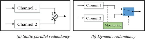
By contrast, Dynamic redundancy, as shown in Figure 1(b), has one channel working in service at a time. The standby channel will replace the active channel only when the other one fails. This scheme obviously requires a monitoring system to check the condition of the channels. An example is an EBHA (Electric Back-up Hydraulic Actuator) actuation system consisting of the integration of one servo-hydraulic actuator and one electro-hydrostatic system as back-up, where the electro-hydrostatic mode will be activated when the hydraulic system fails in service [7].

Considering the redundancy of actuation system for active steering in the railway vehicle, we adopt the principle of dynamic redundancy. However, in this paper, monitoring and detection system is not our research point and we simply assume a suitable fault detection system is available to provide information about an actuator.

2.2. Discussion on actuator technologies

There are different actuation technologies, such as Hydraulic Servo Actuator (HSA), Electro-Hydrostatic Actuator (EHA), Electro-Mechanical Actuator (EMA), Electro-Magnetic actuator etc. Considering the features of mechanical size, energy efficiency, dynamic performance and technical maturity, HSA, EHA and EMA may be the most three attractive technologies and the first two are absolutely dominating technologies so far applied in modern civilian aircraft [14,15].

HSA is a ‘conventional’ hydraulic actuator developed to achieve the concept of ‘Fly-by-Wire’. In HSA, a centralised pump provides a constant pressure of hydraulic oil and then a servo-valve controls the direction and flow rate of the oil so that the reference motion of the cylinder is realised. Power is supplied to the system through the pump continuously, regardless of the reference assigned to the cylinder, and is transferred via pressurised hydraulic oil through a pipeline to the cylinder. HSA is presently the most commonly used technology in aircraft because of its high power density, technological maturity and fail-safe capability as it enables the isolation of a failed hydraulic actuator that can be set in a standby mode through the operation of the standby valve.

The appearance of EHA enables the technology development from ‘Fly-by-Wire’ to ‘Power-by-Wire’. In this case, power is generated in a localised servo motor driving the pump to generate flow rate and pressure gain so that the movement of the cylinder can be controlled. For an Electro-hydrostatic Actuator with a Fix Displacement Pump (EHA-FD), the ideal movement of the cylinder can be achieved accurately by the control of the motor. EHA, deemed as a transition technology between HSA and EMA, can save weight of the actuation system since the localised power supply allows removal of the pipeline network, as well as the valve and reservoir.

While considering the development tendency of More Electric Aircrafts (MEA), EMA as a full electrical actuation system has more potential in the future with respect to the previous two technologies. It allows the removal of valves and pump, further reducing the weight and allowing smaller size. Furthermore, electronic components are easier to be monitored and maintained than hydraulic components, with benefits in terms of vehicle maintenance and availability. However, the limited application of EMA so far has been adopted in civilian aircraft. The cautious utilisation of EMA is due to the lack of technological maturity. The critical issue impairing the diffusion of EMA is the critical effect of a mechanical jam failure mode which may be a result of the malfunction of the ball screw mechanism. Due to this intrinsic mechanical structure, this failure mode is difficult to overcome although some solutions are being investigated [8]. It is worthy of mentioning, however, that EMA is successfully in use for tilt actuation in some series of the Pendolino tilting train [16,17].

According to the above analyses, EMA would be a favourable choice if the safe-critical issue can be solved properly. However, a relative conservative technology roadmap for rail vehicle active primary suspension might start with using HSA and EHA and gradually move to EMA when it is further enhanced towards full suitability for safe-critical applications. In this work, HSA and EHA technologies are considered in the active steering schemes.

2.3. Fault-tolerant schemes for active steering system

The mechanical layout of active steering is to replace the traction rods with actuators. In order to improve the fault tolerance of active steering system, nine practical schemes are defined, labelled with ‘A1, A2, … , C3’ as shown in the three-by-three matrix in Figure 2. The schemes labelled with ‘A’ adopt HSA system and the schemes marked with ‘B’ and ‘C’ implement EHA. For schemes ‘C’, the number of applied actuators is halved by placing controlled actuators only at one side of the wheelset and passive linkages are used to move longitudinally the axle box on the other side. In the linkage, the longitudinal short rods attached to the axle-boxes can rotate with respect to x, y and z axes, while the long lateral rod rotates around the z axis with a rotation point attached to the bogie. The consideration of schemes ‘C’ helps us to understand the influence of reducing actuator number in terms of system reliability. For schemes ‘A’ and ‘B’, the maximum actuation force is assumed to be 20 kN, while for schemes ‘C’, it is doubled to 40 kN, as each actuator has to move two wheels.

Figure 2. Schematic diagram of the proposed nine active steering schemes.

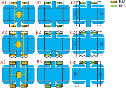
The schemes in the first row do not include either redundancy of actuators or passive back-up. They are, therefore, the simplest configuration for the schemes in the same column. The schemes in the second row labelled with ‘2’ have a passive spring in parallel with each actuator, as a back-up to enhance fault tolerance. However, in these cases, the higher actuation force is required to cancel out the action of passive springs, or otherwise the steering effect could be weakened. The schemes in the third row with ‘3’ have redundant actuators. One actuator will work in active mode and the other one will work in standby mode unless the failure of the first actuation system is detected.

The proposed nine fault-tolerant schemes are in general practical solution considering the possible size of actuators [18] and installation space in primary suspension. The representative nine schemes reflect three directions to improve the fault tolerance, i.e. adding paralleled passive springs; implementing redundant structure as the back-up of the system and reducing the number of actuators by using more reliable mechanical structures. In practice, various fault-tolerant designs can be derived based on these principles, for instance another scheme presented in Figure 12 at the end of the paper.

In the following sections, the steering effects of the nine schemes are briefly compared in Section 3.4. Our research mainly focuses on their fault-tolerant performance which is discussed in Section 4 and Section 5.

3. Modelling of actuation system and vehicle dynamics

3.1. Modelling of actuation system

The dynamic models of HSA and EHA are built in Simulink using Sim-scape. For the brevity of the paper, we only present some key parts of the mathematical models to help understand the modelling work. More details about the modelling of HSA and EHA can refer to the user guidance of Simulink Sim-scape [19].

• (1) Modelling of HSA

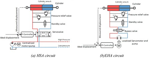
The circuit of the HSA model is illustrated by the schematic diagram in Figure 3(a). It mainly consists of a double-acting hydraulic cylinder, servo-valve, standby valve, hydraulic pipeline and centralised motor and pump. The motor and pump maintain constant high pressure and low pressure levels in two branches of the pipeline network shown in red and blue colour, respectively. Oil flow in the chambers of the cylinder is controlled by a ‘3-position 4-way’ servo-valve in which the movement of the spool is proportional to the input signal and hereby the opening area of orifice and path of hydraulic oil are controlled. Pressure relief valves are arranged to avoid extremely large pressure. When the standby-valve is activated, the actuation works in standby load and no actuation force will be generated. This valve is designed for redundant actuation system.

Figure 3. Schematic diagram of (a) HSA circuit and (b) EHA circuit.

In each actuator, the difference between the reference displacement and the measured displacement is sent to a Proportional + Integral (PI) controller, and the output signal is generated to control the movement of spool so that the actuator can follow the reference displacement. In a real control system for actuators and steering system, some other nonlinear features and system uncertainties could be involved, and multiple targets could be realised at the same time, for instance improving vehicle stability and curving behaviour simultaneously. A more advanced robust control would be useful in this case, see references [20–22]. However, the simple PI controller considered here is fully adequate to perform the study of fault tolerance for an application involving only active steering.

The maximum force and moving speed of the cylinder, as two basic specifications are briefly explained hereinafter in the design of parameters setting. The maximum force of the cylinder $F_{\text{max}}$ is realised by setting piston area A and differential value between high pressure $P_h$ and low pressure $P_l$, as seen in Equation (1). (1) $F_{\text{max}}=A\cdot =(P_h-P_l)=A\cdot \mathrm{\Delta }P$(1) Once the piston area A is defined, the maximum moving speed of the cylinder $v_{\text{max}}$ is derived from the maximum available flow rate, i.e. $v_{\text{max}}=q_{\text{max}}/A$. Equation (2) establishes a relation between $q_{max}$ and the maximum opening area of the orifice $a_{\text{max}}$ of servo-valve. In this equation, the characteristics of fluid oil and servo-valve are involved, including flow discharge coefficient $C_d$, fluid density $\rho$ and turbulent flow $p_{cr}$. (2) $q_{\text{max}}=C_d\cdot a_{\text{max}}\sqrt{\frac{2}{\rho }}\cdot \frac{\mathrm{\Delta }P}{{(\mathrm{\Delta }{P}^2+p_{cr}^2)}^{1/4}}$(2)

The $p_{cr}$ can be calculated according to Equation (3), (3) $p_{cr}=\frac{\rho }{2}{\left(\frac{R{e}_{cr}\cdot \nu }{C_d}\sqrt{\frac{\pi }{4a_{\text{max}}}}\right)}^2$(3) where $R{e}_{cr}\text{ and }\nu$ are, respectively, the critical Reynolds number and fluid kinematic viscosity.

Some key parameters for this HSA model are listed in Table 1.

• (2) Modelling of EHA

Table 1. Key parameters of the hydraulic circuit.

Parameter	Value [unit]
Maximum actuation force $F_{\text{max}}$ (Design target)	20 [kN]
Piston area $A$	$5\times {10}^{-3}[m^2]$
Piston stroke (Single side) $L_p$	$10$[mm]
High pressure $P_h$	50 [bar]
Low pressure $P_l$	10 [bar]
Maximum moving speed $v_{\text{max}}$ (Design target)	20 [mm/S]
Discharge coefficient $C_d$	0.7
Fluid density $\rho$	880 [kg/m^3]
Critical Reynolds number $R{e}_{cr}$	12
Fluid kinematic viscosity $\nu$	$32\times {10}^{-6}[{\text{m}}^{\text{2}}\text{/s}]$
Maximum opening area of the orifice $a_{\text{max}}$	$1.5\times {10}^{-6}[{\text{m}}^{\text{2}}]$

The circuit of EHA is schematically shown in Figure 3(b). In comparison to HSA, the controllable component in the EHA is a localised servo-motor and pump, rather than servo-valve. The outputs of the motor, including the rotating direction and torque, can be controlled by voltage signals. In the EHA model, the control command is firstly converted in a Pulse Width Modulation (PWM) signal and then sent to an H-bridge to drive the DC motor. The bypass valve will be switched on when the vehicle runs through a curve and off when the vehicle runs on a tangent track.

In the steady-state situation, the relationship between the driven voltage $V$ and output torque $T$ can be simplified, as shown in Equation (4). (4) $T=k_t\frac{(V-k_v\omega )}{R}-J\dot{\omega }-\lambda \omega$(4) The product of Back-emf constant $k_v$ and motor rotating speed $\omega$ is the back emf. $R$ denotes armature resistance and $k_t$ represents the torque constant. $J$ and $\lambda$ reflect mechanical features rotor inertia and rotor damping, respectively.

For the fixed-displacement pump model, with the assumption of no friction torque and flow leakage, the pressure gain $\mathrm{\Delta }P$ between two ports of the pump can be calculated according to Equation (5). (5) $\mathrm{\Delta }P=\frac{T}{D}$(5) where $D$ $[{\text{m}}^{\text{3}}\text{/rad}]$ is the fixed displacement of the pump.

Apart from the servo-motor and pump, the hydraulic parts of the EHA share the similar components and parameters with the HSA model. According to Equations (1), (4) and (5), the actuator can be designed to produce the desired maximum actuation force. The parameters adopted for the EHA are listed in Table 2.

• (3) Simulation test for HSA and EHA models

Table 2. Key parameters of the electrical circuit in EHA.

Parameter	Value [unit]
Voltage $V$	48 [V]
Back-emf constant $k_v$	0.17 [V/rad]
Torque constant $k_t$	0.17 [NM/A]
Armature resistance $R$	1.7 [Ω]
Armature inductance $L$	$2\times {10}^{-3}$ [H]
Fixed displacement of pump $D$	$1.2\times {10}^{-6}$ [m^3/rad]
Rotor inertia $J$	$5\times {10}^{-4}$ [kg/m^2]
Rotor damping $\lambda$	$2\times {10}^{-4}$ [Nm/(rad/S)]

Before the integration of the actuation system and vehicle dynamics model, simulation is performed to test the behaviours of HSA and EHA models, where one side of the actuator is mounted on a fixed point and the other side is connected in series with a spring. The stiffness of the spring is 3 MN/m and it is connected to a fixed point on the other side.

A piecewise linear reference displacement is created and the simulated displacement is compared, as shown in Figure 4(a). For both HSA and EHA models, fast response of actuation is observed and satisfactory displacement is found with very minor error in the first 15 seconds when the maximum reference displacement is set to 6 mm. In the last 5 seconds, the reference displacement increases to 8mm and then a significant deviation is observed. This error is due to the limitation of the maximum actuation force 20 kN, which, in turn, validates our parameter setting for force limitation.

Figure 4. Time history of (a) actuator displacement and (b) actuator force of HSA and EHA.

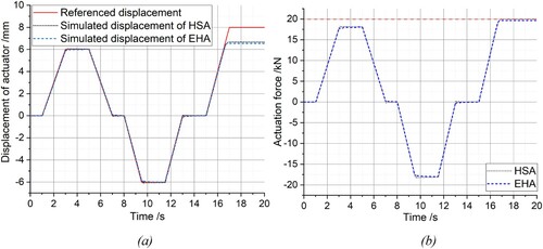
For the fault-tolerant schemes ‘C’, the maximum actuation force is configured as 40kN. We increase the voltage $V$ and decrease Armature resistance $R$ to meet this design value.

3.2. Modelling of vehicle dynamics

The model of the actively controlled vehicle is the integration of the passive vehicle model and the active steering model presented in Section 3.1. The passive vehicle model is built in SIMPACK based on a real inter-city trailer vehicle with a targeted maximum service speed of 160km/h. This model has one car-body, two bogies and four wheelsets. For the passive primary suspension, one coil spring at the top of each axle-box carries the vertical load and provides a small part of the yaw and lateral primary stiffness, while the traction rod, mounted between the axle-box and bogie side beam, transfers the longitudinal force and provides the main part of the yaw stiffness. In secondary suspension, air springs are implemented to produce soft stiffness, and each bogie has one lateral damper, two vertical dampers and two yaw dampers. The mass properties and passive suspension parameters were examined and adjusted by a group of experts in project RUN2RAIL to make the model representative. The major parameters of the passive vehicle model are presented in Table 3.

Table 3. Parameters of the bogie vehicle.

Parameters of the vehicle dynamics model	Value [unit]
Axle load (tare condition)	11[t]
Wheelbase	2500 [mm]
Base of bogie	16 [m]
Diameter of wheel (new)	860 [mm]
Wheel and rail profile	S1002/UIC60
Rail cant	1:40
Mass of car body	30 [t]
Mass of frame	3 [t]
Mass of wheelset	1.8 [t]
Stiffness of primary coil spring in x/y direction	1.2 [MN/m]
Stiffness of primary coil spring in z direction	1.2 [MN/m]
Stiffness of airspring in x/y direction	0.15 [MN/m]
Stiffness of airspring in z direction	0.25 [MN/m]
Longitudinal stiffness of traction rod (Passive scheme)/ Longitudinal stiffness of actuator bushing (Active scheme)	10 [MN/m]/ 50 [MN/m]
Secondary vertical damper	30 [kN/m/s]
Secondary lateral damper	60 [kN/m/s]
Secondary anti-hunting damper	200 [kN/m/s]
Equivalent stiffness of anti-roll bar	1.5 [MN/rad]

In the passive vehicle model, the longitudinal stiffness of the traction rod is 10MN/m, while for the actively controlled vehicle the traction rods are replaced by actuators. A stiff spring (50MN/m) is modelled in series with each actuator to simulate bushing compliance. For schemes A2, B2 and C2, the stiffness of spring in parallel with the actuator is 5MN/m.

3.3. Control strategies for active steering

The so-called perfect-steering control strategies, based on longitudinal creep force, are investigated theoretically in [4,23–25], but these schemes require complex measurements, for instance the conicity of the wheel/rail couple, which are difficult to obtain. In this work, we adopt a practical control strategy that still provides satisfactory steering behaviour [26]. This control strategy is based on the radial position taken by the wheelsets, which can be seen in Figure 5.

Figure 5. Control principle of active steering. (a) Radial position of two wheelsets in curve. (b) absolute yaw angle of bogie.

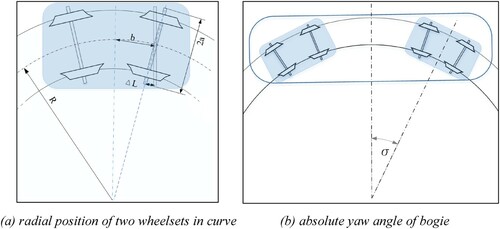
To create a radial position of the wheelset, the ideal displacement of actuator $\mathrm{\Delta }L$ is calculated according to Equation (6) (6) $\mathrm{\Delta }L=\frac{b}{R}\cdot a$(6) where $b$ represents the half wheelbase, and $a$ is the half distance between the right and left actuators; 1/R is the track curvature, which can be obtained by Equation (7): (7) $R=\frac{V}{\dot{\sigma }}$(7) where $V$ denotes the longitudinal speed of the vehicle and $\dot{\sigma }$ is the absolute yaw angular velocity (yaw rate) of the bogie, see Figure 5(b). Based on parameters of our vehicle model, the reference displacement of the cylinder, from Curve R200 to Curve R1000, ranges from 6.6 mm to 1.3 mm.

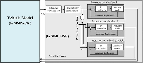
Since the track irregularity introduces the noise of measured signals of $V$ and $\dot{\sigma }$, a low-pass filter is applied to extract the real track layout information, but this will also cause a time delay when a vehicle enters curve transition parts. To alleviate the effect of this delay, a precedence control method, which has been applied in titling trains [16], is adopted here. The signal measured for leading wheelset is delayed by a proper amount of time, considering vehicle speed, distance between axles and delay caused by the low-pass filter and is then applied to the following wheelsets. Unfortunately, this method is inherently not capable of compensating delays in the leading wheelset of the vehicle. The schematic diagram of the control strategy is illustrated in Figure 6.

Figure 6. Schematic diagram for steering control scheme.

3.4. Simulation of vehicle model with actuation system

According to the above description, multi-body simulations are performed on a short-radius curve R250 at 72.7 km/h with non-compensated lateral acceleration (NLA) 0.65 m/s². The curve transition length is 100m and here the track irregularity is not applied.

Figure 7 compares the wheelset angle of attack, track shift force, wear number and derailment between the passive scheme and active scheme A1. Wear number [N] is calculated as follows: (8) $\text{Wear number}=|T_x{v}_x+T_y{v}_y+M_z{\phi }_z|$(8) where $T_x$, $T_y$ and $M_z$ are longitudinal creep force, lateral creep force and creep torque; $v_x$, $v_y$ and ${\phi }_z$ are longitudinal creepage, lateral creepage and spin, respectively.

Figure 7. Time history of the (a) Angle of attack of wheelsets with Passive scheme (left) and with Active steering scheme A1 (right). (b) Track shift force of wheelsets with Passive scheme (left) and with Active steering scheme A1 (right). (c) Wear number of wheelsets with Passive scheme (left) and with Active steering scheme A1 (right). (d) Derailment coefficient of wheels with Passive scheme (left) and with Active steering scheme A1 (right), for the vehicle running in a curve R250.

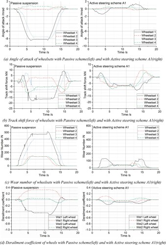
When active steering is applied, the attack angle of all the wheelsets reduces to a very small value, close to zero. This small value comes from the yaw angle of the bogie frame, and provides a nearly equal amount of lateral creepage and creep force which is needed to balance the uncompensated centrifugal force in curves. Two waves are observed for the leading wheelset when it runs through the transitions. This is due to the delay effect of the low-pass filter, as explained in Section 3.3. In Figure 7(b), the track shift forces of all wheelsets of the active vehicle tend to be equal so that the maximum force is reduced from 16 to 7 kN. Owing to the ideal position of the wheelset, the wear number and derailment coefficient are significantly reduced as well. In general, the active steering scheme can provide satisfactory curving performance.

The analysis is repeated for the other actuation schemes and the results are summarised in Table 4. For active schemes A1, B1, C1, A3, B3 and C3, the curving performance is very similar, despite the different number and type of actuators featured by each scheme. However, schemes A2, B2 and C2 are less effective due to the existence of paralleled springs, which cancel out a part of actuation force so that the steering system is unable to correctly realise the required yaw angle of the wheelsets. The decrease of performance for these schemes depends on the maximum actuation force, the longitudinal stiffness of the passive springs and the radius of the curve.

Table 4. Steady-state curving parameters for the passive vehicle and nine active steering schemes.

	Attack angle [mrad]	Track shift force [kN]	Derailment	Wear number [N]	Wear number reduction
Passive	8.18	16.33	0.44	474.89	/
A1	0.38	7.27	0.09	43.30	90.88%
B1	0.40	7.64	0.08	45.68	90.38%
C1	0.35	7.93	0.09	45.88	90.34%
A2	1.20	12.04	0.20	112.48	76.31%
B2	1.26	12.04	0.21	115.60	75.66%
C2	2.11	11.45	0.27	158.27	66.67%
A3	0.38	7.27	0.09	43.29	90.88%
B3	0.40	7.64	0.08	45.69	90.38%
C3	0.34	7.93	0.09	45.88	90.34%

4. The methodology for fault-tolerant analysis

In this section, we propose an approach to analysing the fault tolerance of active steering system where the concept of Risk Priority Number (RPN) from Failure Mode and Effect Analysis (FMEA) is adopted [27].

4.1. Failure mode and effect analysis and risk priority number

Failure Mode and Effect Analysis is a systematic method for evaluating the potential failure modes of the system and their effects. It was firstly proposed for the design of aircrafts and now has been applied in many other industries to reduce the impacts of failure and to improve the reliability of the system. In FMEA, a core concept is to calculate Risk Priority Number (RPN, also called Criticality in [6]) which involves two essential factors: the Severity of the failure in terms of economic losses and injury to people, the Occurrence defined as the likelihood that the failure will take place and a third optional element: the Detectability defined as the ability to detect the failure modes by means of a monitoring system. As shown in Equation (9), the RPN is calculated as the multiplication of the Severity, Occurrence and Detection parameters. (9) $\text{RPN}=\text{Severity}\times \text{Occurrence }(\times \text{Detection})\text{.}$(9)

In the context of active suspension design, all possible failure modes have to be identified and, if the RPN exceeds a threshold value, the system’s design process needs to be modified to reduce the failure mode’s RPN. The approach to defining the value of severity and occurrence is explained in Section 4.3.

4.2. Typical failure modes of actuation system

Although different actuation technologies have various principles and components, their failure modes can be grouped in a limited number of categories which are weak depending on the actual implementation of the steering system. References [6,13] summarise failure modes of actuation systems and the categorisation proposed in the two works is, to a large extent, consistent, as summarised in Table 5. The table applies all kinds of actuator technologies, but ‘Jamming’ is intrinsically related to a fault in the ball screw and therefore shall be considered only for EMAs.

Table 5. Summary of failure modes.

Failure modes summary in Ref. [6]		Failure modes summary in Ref. [13]
1	Hardover	1	Maximum/Min force
2	Fail open	2	Zero force
3	Jamming (EMA)	3	Jamming (EMA)
4	Erratic operation	4	Harmonic excitation
		5	Inverse control
		6	Random excitation
		7	Impulse

Considering the application background of active steering and actuation technologies applied in this work, we present three failure modes that are possibly the most dangerous cases in real service.

• (1) Inverse control

In Inverse control, the produced actuation force is applied in the opposite direction with respect to the one corresponding to the correct operation. This error may arise from the controller, which produces inverse commands, and all the actuators would work in the wrong direction or it could be due to wrong installation or conditioning of sensors or actuators. We study this failure only in curves since this fault will not affect the running of the vehicle in tangent track, given that the no steering command is applied in this latter case.

• (2) Maximum force

The incorrect signals of controllers and sensors may lead to actuation, operating in maximum force to push or pull the wheelset. It can happen in one actuator or in all actuators at the same time. Under this fault condition, the derailment and track shift force on both curves and tangent track are expected to increase. In the simulation, we assume the worst situation that in curves the maximum force is applied in the opposite direction of the right force.

• (3) Zero force

Zero force failure mode means no force is generated by the actuator. When actuation force is missing, the lack of longitudinal stiffness could cause the instability of the vehicle when it runs at a high-speed range. This situation can be caused by a mechanical failure of the cylinder or by a severe leakage in the pipeline or in the cylinder. The loss of power supply or the failure of centralised motor and pump may also lead to the failure of all the actuators in this mode. Besides, the wrong position of the standby valve could produce zero actuation force as well.

According to the above analyses, ten cases are considered, as summarised in Table 6. For each case, the RPN is evaluated for all the active steering schemes in Figure 2 and a comparative analysis is performed in the following sections.

Table 6. Ten Cases for failure mode analysis.

Failure type	Failure configuration of actuation	Tangent track	Curve R250
Inverse control	1 group of Actuator (Leading wst.)	✗	✓
	All	✗	✓
Max force	1 Actuator (Front Left)	✓	✓
	All	✓	✓
Free (Zero force)	1 Actuator (Front Left)	✓	✓
	All	✓	✓

4.3. Severity level estimation

In order to define in an objective way the Severity level, a method, based on the simulation of the vehicle’s running behaviour in the presence of a fault, is adopted here. The method consists of two steps: firstly, the behaviour of the vehicle in the faulty condition is simulated using the MBS (Multibody Simulation) model and a severity factor s is defined comparing the value of safety indicators obtained from the simulation to their limit values in EN14363 [28]. Then, the severity factor is converted into a natural number between 1 and 10 to make it suitable for use in the FMEA analysis.

The two assessment quantities considered are the track shift force $\sum Y_{\text{max}}$ and the derailment coefficient $(Y/Q{)}_{\text{max}}$ which form the basis for safety verification according to EN 14363. The detailed definitions, filtering methods and limits values of the two factors can be found in this standard. When a failure occurs in an active suspension, the increase of the assessment quantities and the remaining margin from the limit value reflect the severity of the failure. Based on this point, the severity factor s is defined as follows: (10) $s(x)=\frac{x^n-F_n^n}{F_l^n-F_n^n}(n=2)$(10) where $F_n$ is the value of safety factor $(\sum Y_{\text{max}}\text{or}(Y/Q{)}_{\text{max}})$ in normal condition; $F_l$ denotes the limit value of safety factor according to EN14363; $x$ represents the factor’s value to be measured in failure condition. An example of simulated derailment coefficient $x$ and corresponding severity factor s is shown in Figure 8, where $F_n$ and $F_l$ are 0.3 and 0.8, respectively. When the constant parameter n is set to 2, the gradient of severity s over x is increasing. It means that the severity factor s will increase more rapidly when factor $x$ approaches to a safety–critical condition. This weighted effect meets the common expectation for severity assessment. The factor s itself can be used as an independent indicator for severity evaluation. When the factor $\sum Y_{\text{max}}$ or $(Y/Q{)}_{\text{max}}$ exceeds the limit value, resulting in a risk for safety, the severity factor s takes values above 1.

Figure 8. Relationship between severity factor s and derailment coefficient.

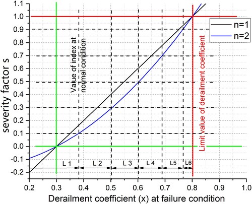
In order to build the connection between the severity factor s and severity ranks for RPN calculation, 10 levels of Severity are defined, as shown in Table 7. Since the limit values of safety factors in EN 14363 are conservative for safety guarantee, the situation of ‘s=1’ is not graded in the top level of severity, but in Rank 7 that starts to have a risk of injured passengers and a small chance of derailment.

Then the Severity level can be obtained for calculating RPN. A method to quantify the Occurrence level is introduced in Section 4.4, whilst Detection is not considered in this work because a realistic estimation of this factor would require the knowledge of the detailed implementation of the steering device together with its monitoring unit.

4.4. Failure occurrence estimation

Although actuation systems have been applied in aircrafts for more than half-century, it is still difficult to estimate the failure rate accurately, let alone the precise estimation for actuation systems to be instead applied in a rail vehicle. Few failure probability data are available for modern actuation systems [29], but the order of magnitude of typical failure modes is presented in [6]. Based on what is available in the references, the failure rates, listed in Table 8, are assumed for different components in the actuation system. These values shall not be considered as highly accurate but still reasonable estimation, at least, of the relative magnitude of failure rates in different components of HSA and EHA systems. In the table, the longer pipeline and more complex servo-valve implied by the HSA lead to higher failure rates assumed for this actuation type, while a higher failure rate of motor and pump is assumed for EHA considering that this actuation system requires the use of a more complex motor and drive.

The idea of Failure Tree Analysis [30] is adopted to calculate the probability of each failure mode. The components associated with the failure modes are marked in Table 9. It is assumed that failures occur independently from each other. The total failure rate for the entire actuator system can be obtained combining the failure rates of the single components according to the following equation: (11) $P_{\text{actuator}}=1-\prod (1-p_{\text{subsystem},i})$(11) where $p_{\text{subsystem},i}$ refers to ith subsystem of the actuator.

Equation (11) is used for calculating failure mode taking place on a single actuator or all actuators. If we consider the vehicle model as a whole system, the calculation of probability should also take into account the number of actuators $n$ for the ‘single’ case, as shown in Equation (12). (12) $P_{\text{vehicle}}=1-(1-P_{\text{actuator}}{)}^n\approx n\cdot P_{\text{actuator}}$(12) Once the probability is estimated, the Occurrence level can be graded, according to Table 10, which is proposed based on empirical data and reference [27]. This table is presented here as an example and it can be adjusted according to the requirement of vehicle operation.

Based on the above methods, the Occurrence level is computed and listed in Table 11.

5. Case studies for typical failure modes

5.1. Examples of failure case study

In this section, the impacts of different failure modes are studied through MBS. The study considers two running conditions for the vehicle: the negotiation of a short-radius curve R250 with speed 72.7km/h (NLA 0.65 m/s²) and tangent track running at maximum service speed plus 10% over-speed which means 176 km/h. For redundant structure, once the monitoring system detects the failure of an actuator, the failed one will be isolated and the back-up actuator will start working. So, if this reaction time is ignored, there will be a negligible difference between the normal case and the failure case. In the following simulations it is assumed that the fault occurs and, if present, the back-up actuator is already activated. The issues of defining in detail how the control system should react to a fault depending on the exact location at which the fault occurs and to consider delays in fault detection remain outside the scope of this paper. Finally, in all simulation cases ORE high-level track irregularity [31] is applied.

Hereinafter, the failure mode Inverse control on all actuators is used as an example for further explanation.

When this failure takes place, the yaw angle and filtered derailment of leading wheelset for schemes A1 A2 and A3 are compared in Figure 9. Due to the inverse control signal, the maximum angle of attack of wheelset for Scheme A1 is doubled compared to the passive case, as shown in Figure 7(a). For Scheme A2, with passive spring in parallel, the yaw angle is lower compared to the faulty A1 scheme, but the benefit in terms of derailment coefficient is limited. For scheme A3, the back-up actuator takes over the role of steering the axle so that both the angle of attack and the derailment coefficient remain basically unaffected compared to the normal case, apart from the effect of track irregularity, see Figure 7. For all cases, the safety factors don’t exceed the limit value.

Figure 9. Time history of the angle of attack and derailment coefficient for the leading wheelset of vehicle running in a curve R250.

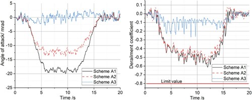
Figure 10 compares the derailment and track shift force (Limit value 46.7 kN) for Inverse control (in all actuators) in all schemes.

Figure 10. Comparison of derailment coefficient and track shift force for Inverse control fault occurring in a curve R250.

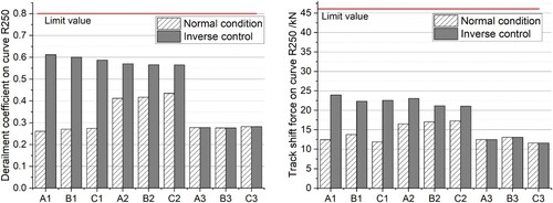
According to these simulation results, the Severity levels are obtained, according to Equation (10) and Table 7. The values are arranged in the form of three by three matrix corresponding to the three by three matrix graphic representation of the actuation schemes shown in Figure 2. (13) ${\mathit{S}}_{\frac{\mathit{Y}}{\mathit{Q}},\mathbf{\text{i}}nverse}=\left[\begin{array}{ccc}4& 4& 3\\ 3& 3& 2\\ 1& 1& 1\end{array}\right]{\mathit{S}}_{\sum \mathit{Y},\mathbf{\text{i}}nverse}=\left[\begin{array}{ccc}2& 2& 2\\ 2& 1& 1\\ 1& 1& 1\end{array}\right]{\mathit{S}}_{\mathbf{\text{i}}nverse}=\left[\begin{array}{ccc}4& 4& 3\\ 3& 3& 2\\ 1& 1& 1\end{array}\right]$(13) The first and second matrix in Equation (13) present the Severity levels based on derailment coefficient and track shift force, respectively. The higher Severity level between the two is selected as representative of the overall assessment and is shown in the third matrix. From these results, the schemes with neither passive spring nor redundant structure have poor effects. The existence of passive springs only brings limited benefit.

Table 7. Description of Severity levels.

Severity factor	Severity rank	Impact	Description
s$<$0.1	1	no impact	No recognisable effect
0.1$\le$s$<$0.3	2	very little	Noticed by a few passengers
0.3$\le$s$<$0.5	3	Little	Impacts on vehicle and infrastructure in the long term
0.5$\le$s$<$0.7	4	very low	Noticed by many passengers
0.7$\le$s$<$0.9	5	Low	Impacts on vehicle and infrastructure in the mid term
0.9$\le$s$<$1.0	6	moderate	Impacts on vehicle and track in the short term
1.0$\le$s$<$1.1	7	High	Risk of injured people and a small chance of derailment
1.1$\le$s$<$1.3	8	very high	Severe impacts on vehicle and infrastructure in the short term
1.3$\le$s$<$1.5	9	very unsafe	Risk of many injured people and a few dead people
s$\ge$1.5	10	catastrophic	Risk of many dead people and the line closed for weeks

Table 8. Failure rates of sub-systems of HAS and EHA ($\mathit{h}\mathit{o}\mathit{u}{\mathit{r}}^{-1}$).

	Sub-system
Failure Rate $p_{subsystem}$	Power supply	(Servo)/Motor and Pump	Cylinder	(Servo)/Valves	Controller	Pipeline	Sensors
HSA	$5\times {10}^{-6}$	$1\times {10}^{-6}$	$5\times {10}^{-7}$	$2\times {10}^{-5}$	$5\times {10}^{-6}$	$5\times {10}^{-6}$	$1\times {10}^{-6}$
EHA	$5\times {10}^{-6}$	$5\times {10}^{-6}$	$5\times {10}^{-7}$	$1\times {10}^{-5}$	$5\times {10}^{-6}$	$1\times {10}^{-6}$	$1\times {10}^{-6}$

Table 9. Parts of the sub-system affecting different failure modes.

	Sub-system
Failure mode	Power supply	(Servo)/Motor Pump	Cylinder	(Servo)/Valves	Controller	Pipeline	Sensors
Inverse control in a group of actuator			✓		✓		✓
Inverse control in all actuators					✓
Max force in one actuator				✓	✓		✓
Max force in all actuators					✓
Zero force in one actuator		✓	✓	✓		✓
Zero force in all actuator	✓	✓(for HSA)

Table 10. Occurrence levels and corresponding failure rate.

Occurrence Rank	Impact	Failure rate [1/hour]
1	Low	P$<$1×10^−7
2		1×10^−7$\le$P$<$1×10^−6
3		1×10^−6$\le$P$<$5×10^−6
4	Moderate	5×10^−6$\le$P$<$2×10^−5
5		2×10^−5$\le$P$<8$×10^−5
6		1×10^−4$\le$P$<2$×10^−4
7	High	4×10^−4$\le$P$<5$×10^−4
8		1×10^−3$\le$P$<1$×10^−3
9	Very high	2×10^−3$\le$P$<2$×10^−3
10		P$\ge 2$×10^−3

Table 11. Occurrence level of different failure modes for the active steering schemes considered in this work.

	Inverse (one)	Inverse (all)	Max force (one)	Max force (all)	Zero force (one)	Zero force (all)
A1	5	4	7	4	7	4
B1	5	4	6	4	6	4
C1	5	4	5	4	5	4
A2	5	4	7	4	7	4
B2	5	4	6	4	6	4
C2	5	4	5	4	5	4
A3	6	4	7	4	7	4
B3	6	4	7	4	7	4
C3	5	4	6	4	6	4

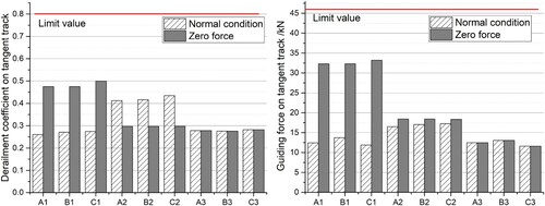
The results obtained for the ‘Zero force’ fault mode taking place in all actuators on tangent track are summarised in Figure 11 and Equation (14). (14) $S_{\frac{Y}{Q},\text{zeroforce}}=\left[\begin{array}{ccc}2& 2& 3\\ 1& 1& 1\\ 1& 1& 1\end{array}\right]S_{\sum Y,\text{zeroforce}}=\left[\begin{array}{ccc}3& 3& 3\\ 1& 1& 1\\ 1& 1& 1\end{array}\right]S_{\text{zeroforce}}=\left[\begin{array}{ccc}3& 3& 3\\ 1& 1& 1\\ 1& 1& 1\end{array}\right]$(14) For this failure case, the paralleled passive springs show significant improvement compared to schemes A1, B1 and C1, due to the fact that when zero force happens at high speed, the vehicle becomes unstable if neither redundant actuators nor a passive back-up is used.

Figure 11. Comparison of derailment coefficient and track shift force for Zero force fault occurring in tangent track.

The other 8 simulation cases are treated in a similar manner and their results are summarised in Section 5.2.

5.2. Simulation results summary and analysis

The Severity levels for all failure modes and simulation cases are summarised in Table 12.

Table 12. Severity levels of different actuation schemes in typical failure modes.

	Inverse (one)	Inverse (all)	Max force (one)		Max force (all)		Zero force (one)		Zero force (all)
Schemes	R250	R250	Tangent	R250	Tangent	R250	Tangent	R250	Tangent	R250
A1	2	4	2	2	4	4	2	1	3	1
B1	2	4	2	2	4	4	2	1	3	1
C1	2	3	2	2	4	3	1	1	3	1
A2	2	3	1	2	2	1	1	1	1	2
B2	2	3	1	1	2	1	1	1	1	2
C2	2	2	1	2	3	1	1	1	1	2
A3	1	1	1	1	1	1	1	1	1	1
B3	1	1	1	1	1	1	1	1	1	1
C3	1	1	1	1	1	1	1	1	1	1

It is clear that implementing a redundant structure is the most effective solution to ensure fault tolerance, regardless of the failure mode considered. The back-up offered by passive springs in parallel can have a significant effect to improve the stability when the ‘Zero force’ failure mode takes place but provides limit improvement for other failure modes. Actuation schemes with no back-up have the worst performance especially for failures happening on all actuators at the same time. Nevertheless, in all fault cases considered, the factors remain below the threshold values of EN 14363. This conclusion, however, cannot be extended to other railway vehicles, because the impacts of the failure modes are not only determined by the specification of the actuation system but also affected by the parameters of the passive suspension, which will differ for different vehicle designs. It shall also be considered that the EN 14363 standard requires that the limit values are compared to 99.85 percentile of the assessment quantity which is obtained from a statistical treatment of at least 20 records obtained from nominally similar running conditions, whilst in this work just one simulation was run for each running condition. The use of the complete statistical processing, prescribed by the standard, would certainly lead to higher values of the safety indicators.

Since the Detection level is not considered in this work, the RPN is obtained as the product of Severity and Occurrence. RPN values are compared for all actuation schemes and running conditions in Table 13. This table clearly reveals the risks of failure modes and also the fault-tolerant capability of different actuation schemes. As expected, the results of the analysis show a more favourable situation for the schemes using actuator redundancy, whilst the actuation schemes with neither passive springs nor redundant structures are significantly worse. However, a sort of ‘grey zone’ is observed in the table, where the RPN values for schemes with a passive back-up are comparable and, for some fault modes, even slightly superior to schemes with full redundancy, thanks to the higher reliability of a scheme using less actuators. Overall, the results open the way to an objective consideration of alternative solutions to meeting fault-tolerant requisites in active steering systems for railway vehicles. It shall be finally mentioned that the analysis reported in this paper does not consider life cycle cost issues, which are, of course, very relevant to the choice of the actuation scheme. From a qualitative point of view, assuming schemes A1, B1 and C1 are ruled out due to fault-tolerant considerations, schemes with a mechanical back-up would provide an advantage compared to solutions with redundant actuators in terms of lower initial purchase cost, but this could be balanced or even overcome by additional maintenance costs in relation to higher wear and RCF damage in wheels and rails due to the sub-optimal steering behaviour of schemes with paralleled springs.

Table 13. RPN values of different actuation schemes in typical failure modes.

	Inverse (one)	Inverse (all)	Max force (one)		Max force (all)		Zero force (one)		Zero force (all)
Schemes	R250	R250	Tangent	R250	Tangent	R250	Tangent	R250	Tangent	R250
A1	10	16	14	14	16	16	14	7	12	4
B1	10	16	12	12	16	16	12	6	12	4
C1	10	12	10	10	16	12	5	5	12	4
A2	10	12	7	14	8	4	7	7	4	8
B2	10	12	6	6	8	4	6	6	4	8
C2	10	8	5	10	12	4	5	5	4	8
A3	6	4	7	7	4	4	7	7	4	4
B3	6	4	7	7	4	4	7	7	4	4
C3	5	4	6	6	4	4	6	6	4	4

In the above analysis, we consider two extreme simulation scenarios, while before the real application, more cases would be expected to cover different vehicle load cases, track layouts and speed profiles.

6. Discussion and conclusion

In this work a quantitative approach was developed to assess the fault tolerance of active steering schemes for railway vehicles, based on MBS simulation to investigate the effect of different possible failure modes. The approach takes advantage of some simplifying assumptions, particularly simplifying the safety assessment based on the consideration of the vehicle’s running behaviour compared to the prescriptions in the European standard EN 14363. Yet, the examples reported show that the process is likely to result in a huge simulation effort, due to the need to consider a variety of possible fault modes in combination with different meaningful running conditions. If a similar method will be applied in the future to design a steering system for a real application, a careful balance will need to be sought between the comprehensiveness and complexity of the analysis. If this goal will not be achieved, there is a serious risk of impairing the use of active primary suspensions in real applications, due to excessive complexity of methods for proving safety and for certification.

Detection and monitoring systems are not considered in this work, but they will play a key role in a real application. For example, EHAs are believed to be easier to monitor than HSAs, as they include more electric/electronic parts but less hydraulic components. In this respect, schemes B and C would show a more favourable case than the results presented in this paper.

For schemes C, the number of actuators is halved compared to other schemes, but a couple of mechanical linkages are introduced. In this work, the occurrence of faults in the additional mechanical linkage was not considered, under the assumption that a proper mechanical design can lead to a negligible failure rate of this component, which is the same assumption usually made for safety-critical parts of standard passive running gear i.e. bogie frames. However, this assumption also depends on the complexity of the component, so the conclusion that the reliability of the system can be improved by replacing active components with passive linkages should be checked for a specific running gear design, a problem not addressed in this paper.

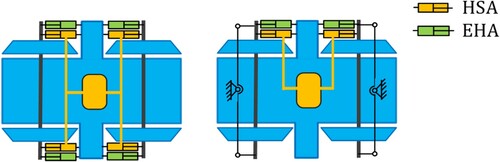
In the evaluation of failure rates for schemes with redundant actuators, the assumption was made that each actuator can work independently. But under some circumstances, the causes that lead to the failure of one actuator may also affect the back-up one. For this reason, redundant actuation system tends to use different control software and different types of actuators for the two channels. In aircraft, the integration of HSA and EHA is adopted as a commonly used scheme. Figure 12 illustrates two other active steering schemes that would be more favourable in respect of this issue compared to A3, B3 and C3 considered in this paper.

Figure 12. Steering schemes alternative to A3/B3 and to C3.

Acknowledgement

The contents of this publication only reflect the authors’ view and the Joint Undertaking is not responsible for any use that may be made of the information contained in the paper. The authors thank Mr Rocco Giossi, Prof. Roger Goodall, Dr Rickard Persson and Prof. Sebastian Stichel for their useful discussions of methods and results throughout this work.

Disclosure statement

No potential conflict of interest was reported by the author(s).

Additional information

Funding

The work presented in this paper has received funding from the Shift2Rail Joint Undertaking under the European Union’s Horizon 2020 research and innovation programme under grant agreement no. 777564.

References

- Goodall RM, Kortum W. Active controls in ground transportation – a review of the state-of-the-art and future potential. Veh Syst Dyn. 1983;12:225–257.
- Goodall RM. Active railway suspensions: implementation status and technological trends. Veh Syst Dyn. 1997;28:87–117.
- Bruni S, Goodall RM, Mei TX, et al. Control and monitoring for railway vehicle dynamics. Veh Syst Dyn. 2007;45:743–779.
- Fu B, Giossi RL, Persson R, et al. Active suspension in railway vehicles: a literature survey. Railw Eng Sci. 2020;28:3–35.
- Perez J, Stow JM, Iwnicki S. Application of active steering systems for the reduction of rolling contact fatigue on rails. Veh Syst Dyn. 2006;44:730–740.
- Maré J-C. Aerospace Actuators 1 Needs, Reliability and Hydraulic Power Solutions. Aerosp. Actuators 1. Wiley; Hoboken; 2016.
- Van den Bossche D, Airbus. The A380 Flight Control Electrohydrostatic Actuators, Achievements and Lessons Learnt. 25th International Congress of the Aeronautical Sciences, Hamburg, Germany. 2006.
- Garcia A, Cusidó J, Rosero JA, et al. Reliable electro-mechanical actuators in aircraft. IEEE Aerosp Electron Syst Mag. 2008;23:19–25.
- Mei TX. A study of fault tolerance for active wheelset control. 22nd IAVSD, Manchester; 2011.
- Mirzapour M, Mei TX, Jin X. Fault detection and isolation for an active wheelset control system. Veh Syst Dyn. 2014;52(suppl):157–171.
- Park J, Shin Y, Hur H, et al. A practical approach to active lateral suspension for railway vehicles. Meas Control (UK). 2019:1–15.
- Umehara Y, Kamoshita S, Ishiguri K, et al. Development of electro-hydraulic actuator with fail-safe function for steering system. Q Rep RTRI. 2014;55:131–137.
- Qazizadeh A., Stichel S., Persson R. Proposal for systematic studies of active suspension failures in rail vehicles. Proc Inst Mech Eng Part F J Rail Rapid Transit. 2018;232:199–213.
- Mare J-C. Aerospace actuators 3 European Commerical aircraft and Tiltrotor aircraft. Hoboken: Wiley; 2018.
- Qiao G, Liu G, Shi Z, et al. A review of electromechanical actuators for more/All electric aircraft systems. Proc Inst Mech Eng Part C J Mech Eng Sci. 2018;232:4128–4151.
- Persson R, Goodall RM, Sasaki K. Carbody tilting - Technologies and benefits. Veh Syst Dyn. 2009;47:949–981.
- Kuka N, Elia A, Ariaudo C, et al. Alstom state of the art on design, simulation and assessment of tilting trains. Dyn Veh Roads Tracks. 2018;2:569–574.
- Research report of project RUN2RAIL, Deliverable 3.1 – State of the art actuator technology. Available from: http://www.run2rail.eu/Page.aspx?CAT=DELIVERABLES&IdPage=06c1be36-4a7a-42e8-9bed-bfe71c3134be. 2018.
- User guidance of Simulink Sim-scape. Available from: https://www.mathworks.com/products/simscape.html.
- Tagawa Y, Ogata H, Morita K, et al. Robust active steering system taking account of nonlinear dynamics. Veh Syst Dyn. 1996;25:668–681.
- Sun W, Pan H, Gao H. Filter-based adaptive vibration control for active vehicle suspensions with electrohydraulic actuators. IEEE Trans Veh Technol. 2016;65:4619–4626.
- Qazizadeh A, Stichel S, Feyzmahdavian HR. Wheelset curving guidance using H∞ control. Veh Syst Dyn. 2018;56:461–484.
- Goodall RM, Mei TX. Chapter 11 of Handbook of Railway Vehicle Dynamics. Boca Raton: CRC Press; 2006. p. 327–357.
- Shen S, Mei TX, Goodall RM, et al. A study of active steering strategies for railway bogie. Veh Syst Dyn. 2004;41(suppl):282–291.
- Pérez J, Busturia JM, Goodall RM. Control strategies for active steering of bogie-based railway vehicles. Control Eng Pract. 2002;10:1005–1012.
- Fu B, Bruni S. Fault-tolerant analysis for active steering actuation system applied on conventional bogie vehicle. 2020. p. 90–99. Available from: http://link.springer.com/https://doi.org/10.1007/978-3-030-38077-9_11.
- EN 60812:2018. Failure modes and effects analysis(FMEA and FMECA)
- EN 14363:2016. Railway applications testing for the acceptance of running characteristics of railway vehicles testing of running behaviour and stationary tests. 2016.
- Bennett JW. Fault tolerant electromechanical actuators for aircraft. 2010.
- EN 61025:2007. Fault tree analysis (FTA). 2007.
- ORE B176: Bogies with steered or steering wheelsets, Report No. 1: Specifications and preliminary studies, Vol. 2, Specification for a bogie with improved curving characteristics, ORE, Utrecht 1989.