
 ?Mathematical formulae have been encoded as MathML and are displayed in this HTML version using MathJax in order to improve their display. Uncheck the box to turn MathJax off. This feature requires Javascript. Click on a formula to zoom.
Abstract
In this paper, we discuss three improved brush models. The first one deals with the coupling between the slip and spin parameters and is valid for relatively high steering speed and small camber angles; the second one is more complex and considers the presence of a two-dimensional velocity field inside the contact patch due to large camber angles; the third one is more general and combines both the previous formulations. For the last two models, the investigation is conducted with respect to a rectangular contact patch, for which we show that three different regions can be identified, each of them corresponding to a different steady-state solution for the deflection of the bristle. Furthermore, from the transient analysis it emerges that each region can be in turn separated into an area in which steady-state conditions reign and another one in which the transient solution takes place. An asymptotic analysis is carried out for the three models and it is shown that the solutions are equivalent to the ones predicted by the standard brush theory for small values of the spin ratio and camber angle. Finally, a comparison is performed amongst the models to highlight the differences in the predicted tyre characteristics.
Acronyms and abbreviations
In the present paper, we use some abbreviations. We sumarise here the main acronyms used throughout the paper:
| Acronym | = | Explanation |
| 1DM | = | One-dimensional brush model |
| 1DCM | = | One-dimensional brush model for coupled slips and spin |
| 2DM | = | Two-dimensional brush model |
| 2DCM | = | Two-dimensional brush model for coupled slips and spin |
| BC | = | Boundary condition |
| IC | = | Initial condition |
| ID | = | Initial data |
| IFT | = | Implicit Function Theorem |
| ODE | = | Ordinary differential equation |
| PDE | = | Partial differential equation |
1. Introduction
Tyres constitute the primary interface between ground vehicles and the environment. Their peculiar behavioural properties allow them to undergo deformations which cause longitudinal and lateral forces to arise inside the contact patch. Thus, a reliable prediction of tyre characteristics is crucial when it comes to real-time optimisation of the vehicle overall performance. Another critical aspect concerns tyre characterisation. Indeed, tyre data can be often collected only under highly controlled conditions, which might be difficult to replicate with precision due to the long and expensive procedures. Also, these tests are mainly carried out on very smooth surfaces which do not reflect the real working conditions.
Accurate tyre modelling has gained a vital importance during the last five decades, and multiple approaches have been proposed depending on the specific application. In particular, the most famous model is the so-called Pacejka's Magic Formula (MF): a wide set of empirical equations which are able to fit tyre characteristics with astonishing precision for different working ranges [Citation1,Citation2]. The MF has been perfected over the years to cover several cases which were not contemplated by the earlier versions, being today the ultimate tyre model. For example, a great deal of research was devoted by both Besselink and Pacejka [Citation3,Citation4] to account for the effect of the inflation pressure and for transients. More recently, Farroni [Citation5–8] integrated the MF description with a full-physical thermal model in order to include the contribution of the tyre temperature. As a result, the MF coefficients have been redefined as temperature-dependent functions. However, the main drawback of MF formulation is that it relies on a large number of fitting parameters, whose physical meaning is not always easy to interpret.
An antipodal description, full-physical tyre models – like FTire [Citation9–11] and CDTire [Citation12] – are instead capable of an accurate description of the local phenomena occurring inside the contact patch. In particular, the bordering on perfection FTire
combines multibody dynamics features with nonlinear curved beam equations and appropriate circumferential extensibility of the tyre, and represents today a standard in the context of advanced driving simulations. Indeed, in spite of their complexities, these models are able to run in real-time. However, simple analytical investigations are merely impossible to conduct because of the extremely detailed modelling.
Other physical theories are based on an exhaustive description of the frictional phenomena which take place in the contact patch. Some of them have been derived from more generalising models employed in the context of tribological studies. Perhaps, the most famous friction-based tyre model is the LuGre [Citation13], initially developed during a collaboration between the Lund and Grenoble universities and then extended by several authors towards disparate applications, including vehicle dynamics and other automotive-related fields [Citation14–20]. In particular, in the LuGre formulation, the planar contact stresses exerted at the tyre-road interface and the friction-induced hysteresis are described in terms of an inertial friction state which can be identified with the deformation of a material point of the tyre tread contacting the ground. The governing equation of the model is a one-dimensional inhomogeneous transport equation, which is usually discretised in space and then solved in time.
On the other hand, brush models [Citation1,Citation2,Citation21–24] represent a more naive but still insightful approach when it comes to a pure physical description of the tyre. They are derived from a simplified version of the classic theory of contact mechanics [Citation25–31], are grounded on few assumptions, and are still accurate enough to reflect the main variations in tyre characteristics due to different operative conditions. Furthermore, the reduced order in the number of required parameters allows for essential speculations about the governing physics of the tyre-road kinematics, providing a deep understanding of the basic phenomena occurring in the contact patch. The underlying idea is that the tyre-wheel system can be assumed to be a rigid body provided with bristles which only deform in longitudinal and lateral direction inside the contact patch. The governing equations are hence expressed in Eulerian form.
In particular, the brush theory was established as main mathematical foundation for tyre modelling since the earliest studies conducted by Pacejka on shimmy phenomena. Indeed, he used the brush theory to investigate the local deformation of string-like models during lateral manoeuvres [Citation32]. Pacejka found that the displacement field of the tyre carcass can be deduced starting from the tyre-road kinematic equations and managed to quantify the generalised forces acting on the wheel hub in the frequency domain. The importance of the brush models has been then consolidated and sometimes revamped over the years thanks to several famous works relating to different fields. For example, Higuchi [Citation33,Citation34] modelled the effect of large camber angles and derived an alternative version of the tyre-road kinematic equations. Takacs [Citation35,Citation36] continued with very remarkable and insightful investigations about shimmy and micro-shimmy related phenomena [Citation37–41], combining brush models with more advanced approaches. Svendenius [Citation42–44] investigated the effect of more realistic shapes of the vertical pressure inside the contact patch and developed a semi-empirical formulation to easily account for the contribution of non-negligible camber angles. Together with other authors [Citation45–47], he used the brush models for the purpose of real-time friction estimation. In his book, Guiggiani [Citation21] redefined the classic science of vehicle dynamics providing a more mathematically rigorous and systematic approach. From a tyre modelling perspective, he emphasised the crucial role played by the brush models because of their physical nature, and analysed the connected transient problem in a very general case. Other authors have studied unsteady-state conditions by using numerical methods [Citation48,Citation49] or proposed enhanced formulations to extend the classic theory towards complex geometries [Citation50,Citation51].
Recently, the authors have developed an exhaustive theory which captures the dynamics of the bristles in the contact patch [Citation52]. A class of simplified formulae has also been introduced to deal with more complex scenarios and take into account the major effects connected with the tyre carcass dynamics.
In the present paper, we extend our previous investigation to analyse a wide class of theoretically unexplored problems. More specifically, we first generalise the classic boundary conditions prescribed by the standard brush theory by expressing them in terms of the inflowing flux. Then, we derive three different models in order of complexity. The first one deals with sufficiently high steering speeds to excite the coupling between the longitudinal and lateral deflections of the bristle and the slip and spin parameters, respectively. This variant of the classic brush model predicts a correlation between the longitudinal deflection and the lateral slip and vice versa, and can be used to reflect working conditions for which the cornering plays a crucial role but the camber angle is instead limited. We refer to this theory as the one-dimensional model for coupled slips and spin (1DCM).
The second model – renamed two-dimensional model (2DM) – is valid for arbitrary large values of the camber angle and deals with the presence of a two-dimensional velocity field inside the contact patch. In this case, the governing equations result in a more complicated formulation. For a rectangular contact patch, we prove the existence of three different regions in which the steady-state solution is given by a different analytical expression. For both the above mentioned models we perform an asymptotic analysis to ascertain that they are equivalent to the classic one for small values of the spin parameter and camber angle, respectively. The last model is the complete one, referred to as two-dimensional model for coupled slips and spin (2DCM), and accounts for both the presence of the coupling between the slips and spin parameters and for a two-dimensional velocity field. Also in this case, we conduct a complete analysis in the case of a rectangular contact shape. The resulting expressions for the deflections of the bristles inside the contact patch show similar features with the ones predicted by both the two previous theories. Since the characteristics equations are the same as for the 2DM, we can also identify the same regions in the contact patch in which the steady-state and transient solution for the bristle displacement assumes a different analytical expression. Finally, an asymptotic analysis is carried out to verify that the 2DCM is consistent with the 2DM for sufficiently small values of the steering speed.
We stress that the models presented in work paper are not intended as an alternative to the classic brush theory, which is sufficient in most of the cases and much easier to implement in simulations. Instead, they can be thought as an effective theoretical foundation to investigate analytically some phenomena which are often studied by means of advanced FEM or multibody models.
This paper is organised as follows: in Section 2, the tyre-road contact equations are presented in the most general form. The definition of the generalised slip quantities is introduced and the main variables and assumptions are explained. In Section 3, the 1DCM is presented. The governing equations are solved for both the steady-state and the transient cases and some comparisons are performed with the results predicted by the classic brush theory. In Section 4, the 2DM is derived and we show some results concerning the shape of the solution for the steady-state problem. The transient solution is also derived and the asymptotic analysis is carried out. In Section 5, the 2DCM is discussed and an analytical solution for the deflection of the bristles in each subdomain of the contact patch is given. Consistency with the 2DM is verified for the longitudinal deflection in the main area of the contact patch. Finally, the main conclusions are drawn in Section 7 and further steps in research are outlined.
2. Tyre-road contact mechanics equations
Let us consider a reference frame Oxyz with unit vectors , whose origin O is located in the centroid of the contact patch; the axes are oriented according to the SAE system: the x axis is directed towards the longitudinal direction of motion, the z axis points downward and the y axis lies in on the road surface and is oriented so that the coordinate system is right-handed. The contact patch is defined mathematically as a closed set
, whose interior and boundary are denoted with
and
, respectively. The contact patch collects all the points
of the tyre which make contact with the road (represented by the Oxy plane). The road is modelled as a perfect homogeneous, isotropic flat surface, without any irregularity.
During the rolling of the tyre, a quantity can evolve over the time or, equivalently, over a peculiar distance
which we call travelled or rolling distance; its meaning will be clarified in the following. In particular, at each point
we associate a three-dimensional speed field
and a finite vector displacement
, which represents the relative deformation of the material point located at the coordinate
with respect to its initial configuration. In the brush model, the deformation of a material point is also interpreted as the deformation of a bristle attached to the tyre; hence, we refer sometimes to the deformation, deflection or displacement of a bristle. Each material point may be also subjected to a force per unit of area, which may vary both in space and time,
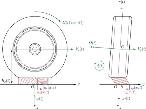
. The whole situation is illustrated in Figure .
Figure 1. Tyre-road schematics in the Oxz and Oyz planes (left and right-hand side figures, respectively). The geometric parameters are drawn in black, the kinematic quantities in green, the generalised forces in blue and the elastic displacements in red. The dimension and the deformation of the bristles have been exaggerated to facilitate the visualisation.
Since we only deal with the planar problem, we consider the tangential (or planarFootnote1) and normal vectors to the road plane, denoted with and
. Accordingly, we also define the tangential velocity field, the tangential displacement vectors and the tangential stress vector as
,
and
, so that
,
Footnote2 and
. Sometimes, in this paper, we also call
shear stress vector.
Finally, we assume that the planar problem can be decoupled from the vertical one; this implies that the vertical component of each quantity defined so far is not influenced by the tangential ones. In particular, we assume that no modification occurs in the original vertical pressure distribution due to friction-related phenomena.
The relative speed between a material point inside the contact patch and the road is called micro-sliding speed indicated with Footnote3 and the tangential micro-sliding speed is defined pertinently as
. Adopting a simple Coulomb friction model, the fundamental equations governing the tyre-road contact mechanics can be now formulated as follows [Citation21]:
(1a)
(1a)
(1b)
(1b) where
and
and
are the static and dynamic friction coefficient, respectively. In general, both can be made dependent explicitly on the vector position
or on the sliding speed
; however, to keep the complexity of the analysis within acceptable levels, here we only use constant values for
and
. For more sophisticated formulations and extensive discussion, the reader may instead refer to [Citation53–55]. There are, of course some limitations connected with the latter simplification. More specifically, Equation (Equation1
(1a)
(1a) ) are only valid under the assumption of memoryless friction, and hence dynamic behaviours due to complex phenomena, e.g. viscoelasticity, are automatically neglected.
To solve the above Equation (Equation1(1a)
(1a) ), two other sets of relations are needed: the tyre-road kinematic equations and the constitutive relations. The first set prescribes a relation between the sliding speed and the deformation of the tyre inside the contact patch; the latter the relation between the aforementioned deformation and the tangential stress acting on each material point.
2.1. Tyre-road kinematic equations
In the present paper, we assume that – from a frictional perspective – there is only one sticking zone (in which the bristles are in adhesion condition) and one sliding zone (in which finite sliding occurs between the bristles and the road, i.e. ) inside the open set
. This is a strong assumption, but leads to an enormous simplification of the problem. Indeed, in this way, the domain in which the partial differential equations (PDEs) ruling the tyre-road kinematics are defined coincides with the interior of the contact patch
, and the corresponding BCs can be formulated uniquely on
. More exhaustive models of friction, which do not rely on the latter simplifying hypothesis, can be found in [Citation16–20,Citation56,Citation57]. It is also worth pointing out that some efforts have been devoted to remove the assumption of a single sticking zone also in the context of the brush theory, for example recently by Guiggiani [Citation21], but the investigation becomes feasible only numerically by means of iterative algorithms. Here we want to conduct an investigation to derive, where possible, a closed-form expression for the tangential deformation
of the bristle, and hence we try to simplify the analysis as much as possible.
The micro-sliding speed reads, in vector form, Pacejka [Citation2], Guiggiani [Citation21], Limebeer and Massaro [Citation23], Romano et al. [Citation24], Romano et al. [Citation52]
(2)
(2) with
(3a)
(3a)
(3b)
(3b)
(3c)
(3c)
(3d)
(3d)
(3e)
(3e)
(3f)
(3f) where
is the macro-sliding velocityFootnote4 and coincides with the velocity of a hypothetical point S representing the projection of the centre C of the wheel hub onto the road plane,
and
are the longitudinal and lateral speed of the wheel hub, whose planar coordinates are given by the vector
,
is the rolling speed of the tyre around its axis,
is the so-called rolling radius,
is the camber angle and
is the steering angular speed. The geometrical radius
denotes the vertical coordinate of the centre of the wheel hub with respect to the reference frame Oxyz. Finally, in the authors' knowledge, the quantities
and
have never been defined in literature; we call them camber and steering ratio, respectively. They represent the contribution of the two components of the angular speed in z direction (the first one due to the camber angle, the second to the steering speed) to the total value of
.
It is crucial to understand that, since we are analysing the tyre-road interaction by means of the Eulerian approach, the total derivative of a quantity is given by . However, since we are only focussing on the tangential problem,
and hence we may instead use
, where
collects the tangential components of the gradient.
With the premises above, Equation (Equation2(2)
(2) ) can be recast in scalar form as
(4a)
(4a)
(4b)
(4b) with
(5a)
(5a)
(5b)
(5b) In the classic brush theory, which deals with a one-dimensional velocity field
, the coupling between the longitudinal and tangential displacement of the bristle is also neglected, i.e.
. We refer to the classic theory simply as one-dimensional theory (1DM). Instead, in the following analysis, we will make different assumptions on the components
and
of the velocity field, as well as on the parameter
, to properly account for different operative conditions of the tyre. The boundary conditions (BCs) for the problem under consideration can be stated inherently depending on the specific structure of the velocity field.
2.1.1. Slip parameters
The solution of the tyre-road kinematic equations simplify if the analysis is conducted with respect to nondimensional quantities, called slip variables or parameters .Footnote5 In this way, the problem can be made independent of the rolling speed of the tyre. Thus, we introduce the theoretical slip parameters reading
(6a)
(6a)
(6b)
(6b) where the quantity
is referred to as rolling speed and the subscript r stands for rolling. The quantities
and
are called longitudinal and lateral slip, respectively, whilst φ is referred to both as rotational slip or spin. We point out that, unlikely many authors which define the spin as
, we have chosen to divide simply by
; in this way,
and
are both nondimensional quantities. For some applications, it may also be useful to define the transientl slip as in [Citation21], which incorporates in its definition the transient deflection of the tyre carcass. Generally speaking, in the following investigations we will neglect the carcass dynamics, even though it heavily affects the transient trend of the forces exerted at the tyre-road interface; this kind of study, however, is out of the scope of the present paper.
Finally, we introduce mathematically the notion of travelled distance as follows:
(7)
(7) In many cases, we will use the travelled distance as independent coordinate in place of the time variable.
2.2. Constitutive relation
In spite of the viscoelastic nature of the tyre, for sake of simplicity it has been commonly established in literature to assume linear elasticity [Citation21], i.e. a constitutive relation of the type
(8)
(8) where the tangential stiffness matrix
is defined as [Citation21]
(9)
(9)
2.3. Boundary and initial conditions
Equation (Equation4(4a)
(4a) ) are two coupled PDEs – more specifically, linear transport equations – defined on a finite open domain
. Thus, to guarantee the uniqueness of the solution, we need to prescribe a BC and an initial condition (IC). To formalise the BCs correctly, it is firstly necessary to define the leading edge
, the neutral edge
and the trailing edge
[Citation58] as
(10a)
(10a)
(10b)
(10b)
(10c)
(10c) where the unit vector
represents the outer-pointing unit normal which lies in the
plane. Note that the scalar product
represents the elementary flux
through the boundary
of the contact patch.
Indeed, the classic brush theory prescribes the continuity of the shear stress at the interface between the free portion of the half space and the interior of contact area. If a pure elastic constitutive relation is assumed, the direct consequence of is that the bristles inflowing into the contact patch must enter undeformed.
The previous boundary can be stated in mathematical terms as
(11)
(11) Basically, the previous relation imposes that the bristles must enter the contact patch undeformed, since the points
are the points inflowing into the contact patch
. Furthermore, we can partition the leading edge as follows
(12)
(12) so that, with the necessary precautions needed to apply the Implicit Function Theorem (IFT), we can find two parametrisations for each subset
, namely
and
, such that we can write
(13a)
(13a)
(13b)
(13b) the BC (Equation11
(11)
(11) ) can be recast as
(14a)
(14a)
(14b)
(14b) Note that the above boundaries with the condition (Equation10a
(10a)
(10a) ) ensure that the boundary data (BDs) are never characteristic (the reader may refer, for example, to [Citation59,Citation60]).
As far as the IC, is concerned, we introduce the additional assumption of vanishing sliding [Citation2], which corresponds to have infinite friction available inside the contact patch, i.e. . By doing this, we can formulate the IC on the whole interior
of the domain
Footnote6:
(15)
(15) for any
. The assumption of vanishing sliding will be eventually removed in Section 6. Another constraint which we introduce is that
. This can be justified by frictional considerations.
3. One-dimensional model for large steering speeds
In this section, we introduce a model which can be applied when the spin parameter is large. This case is relevant when the contribution of the steering speed is non-negligible, but the camber angle is sufficiently small to be disregarded (). We refer to this model as the one-dimensional model for coupled slip and spin (1DCM). The reason for such a definition is that, as it will be highlighted in the following, large spin values excite a coupling between the slip and spin parameters. Another assumption which we introduce is that all the geometric quantities, the speeds and the slip parameters in Equations (Equation3
(3a)
(3a) ) and (Equation6
(6a)
(6a) ) are constant over the time. Owing the premises above, the tangential velocity field can be approximated by the rolling speed as
, so that
(16a)
(16a)
(16b)
(16b) In the regions of the contact patch where no sliding occurs (i.e.
), we can recast Equation (Equation16
(16a)
(16a) ) as
(17a)
(17a)
(17b)
(17b) where we have introduced the new coordinate system
(18)
(18) and replaced the time variable with the travelled distance
. The variable ξ is often referred to as distance from the entrance and represents to the longitudinal coordinate measured from the leading edge. Indeed, the quantity
represents the position of the leading coordinate at the lateral position y (η).
Since, for the case under consideration, the velocity field is one-dimensional, the BC (Equation14(14a)
(14a) ) and the IC (Equation15
(15)
(15) ) can be reformulated respectively as follows:black
(19)
(19)
(20)
(20) Solving (Equation17a
(17a)
(17a) ) for
and substituting into (Equation17b
(17b)
(17b) ) yields
(21a)
(21a)
(21b)
(21b) Equation (Equation21b
(21b)
(21b) ) is a parabolic second-order PDE, which can be reduced to its canonical form by a proper transformation of variables. In particular, performing the coordinate change
,
change, Equation (Equation21b
(21b)
(21b) ) turns into
(22)
(22) whose solution reads, in terms of
and s,
(23)
(23) Imposing the BC (Equation19
(19)
(19) ) yields the following expression for the displacement vector
for
:
(24a)
(24a)
(24b)
(24b) At this point, some elucidation is needed. We said that large values of the steering speed imply a coupling between the slip parameters (
and
) and the spin φ. By looking at Equation (Equation24
(24a)
(24a) ), this is clear: φ appears in the denominator multiplying both the slip quantities, and also as argument of the trigonometric functions (note that the nonlinear terms are always given by the product of the longitudinal or lateral slip in turn with some function of φ, but never between the translational slips). This effect is not predicted by the classic 1DM, where the bristle displacement is linear in
,
and φ. Furthermore, in the 1DM, the longitudinal component of the deflection depends only on the longitudinal slip and spin,
and φ, whereas the lateral deflection is only a function of
and φ.
The transient solution for (Equation21b(21b)
(21b) ) can be computed by performing the second coordinate change
,
, to obtain
(25)
(25) whose solution reads, in terms of ξ and s,
(26)
(26) Imposing the IC (Equation20
(20)
(20) ), we get the expressions for the transient deflection
of the bristle for
:
(27a)
(27a)
(27b)
(27b) Similar considerations about the coupling between the slip and spin parameters can be drawn for the transient deflection. In particular, it can be noted that the overall structure of the solution is similar to the one of the steady-state deformation of the bristle, with the difference that the longitudinal coordinate ξ is replaced by the travelled distance s in the trigonometric functions.
3.1. Asymptotic analysis
The previous analysis shows that, for sufficiently large values of and φ, the global solution
is nonlinear in the slip and spin parameters and also every component of the tangential displacement depends on both
and
. Thus, we need to ascertain that Equations (Equation24
(24a)
(24a) ) and (Equation27
(27a)
(27a) ) are equivalent to the linear expressions predicted by classic 1DM for small values of
and φ. These formulae can be found in many books, although here we refer explicitly to the notation used in [Citation52]. We start from Equation (Equation24
(24a)
(24a) ) by expanding the trigonometric functions in Taylor series up to the second term to get
(28a)
(28a)
(28b)
(28b) and neglecting the linear and higher-order terms in
and the quantities
,
yields
(29a)
(29a)
(29b)
(29b) which are identical to the formulae derived in [Citation52]. It can be immediately observed that, in (Equation29
(29a)
(29a) ), both
and
are linear functions of
,
and φ and also
does not depend on the lateral slip and vice versa.
Similarly, we perform the series expansion for the transient solution as follows:
(30a)
(30a)
(30b)
(30b) and neglecting again the terms in
and the displacements
and
we get after some algebra
(31a)
(31a)
(31b)
(31b) which, again, correspond to the transient solutions found in [Citation52].
It is worth noting that, even though we needed to expand into Taylor series up to the second order, we then neglected the terms in and
. This indicates that the classic 1DM is very precise only for very small values of
, since the highest committed error is in the order of
(being always
). Of course, this is the case in most vehicle dynamics applications and the two solutions are eventually indistinguishable.
4. Two-dimensional model for large camber angles
The model developed in this section is valid when the camber angle is sufficiently large to generate a non-negligible component of the rolling speed in y direction. However, we consider the case in which the component due to the steering speed is small enough to neglect the coupling between the longitudinal and lateral deflections of the bristle (). Also, we assume that the longitudinal component of the velocity field is always negative, i.e.
, which leads to the following conditions
(32a)
(32a)
(32b)
(32b) The previous inequalities are fundamental when looking for a particular solution of the problem (see Appendix 1). From a physical perspective, this mathematical requirement states that the tyre semiwidth must be smaller than the lateral coordinate at which the wheel axis intercepts the ground. Of course, in reality this condition is always fulfilled. Another constraint which we impose is that the longitudinal coordinate of the wheel centre must be small if compared with the contact patch length, i.e.
. Finally, the geometric and slip parameters are again assumed to be constant over the time.
Owing the previous assumption, Equation (Equation4(4a)
(4a) ) can be restated as follows in the adhesion region:
(33a)
(33a)
(33b)
(33b) where
(34a)
(34a)
(34b)
(34b) are the longitudinal and lateral components of the velocity field
. In the following, we derive the solutions for the deflection of the bristles for the case of a rectangular contact patch
, where l is the contact patch length and w is the width. Albeit not a very realistic shape for cambered tyres – especially motorcycle tyres, for which large cambering manoeuvres can take place – we consider a rectangular contact shape for two main reasons. The first one relates to the fact that an analytical solution might not be possible for complex geometries; the second one is that the rectangular contact shape is often adopted when dealing with the 1DM, and, as previously done with the 1DCM, we want to establish a possible connection with the 1DM by means of the asymptotic analysis to show a consistency with the results already known in literature.
Recalling the general form of the BC (Equation11(11)
(11) ), for a rectangular contact patch we can restate them specifically as
(35)
(35) Indeed, owing the assumption
, the longitudinal component of the velocity field will be always negative. Hence, all the points located at
will be inflowing into the contact patch. This can be stated in mathematical terms as
(36)
(36) However, for the case under consideration, we have a two-dimensional velocity field, which means that the bristles can also enter the contact patch from the lateral edges, located at
and
, respectively. More specifically, as far as the lateral component
is concerned, we can note that, for
,
and
. Vice versa if the camber angle is negative, i.e.
. In formulae:
(37)
(37)
(38)
(38) In the subsequent analysis, we will show that, because of the three different boundary prescriptions, it is possible to identify three subdomains the contact patch is partitioned in, which we denote with
,
,
, respectively. These regions correspond to three different analytical expressions for the steady-state deformation of the bristle. Furthermore, as for the classic 1DM and 1DCM, the steady-state and the transient problems can be decoupled since the space boundaries prescribe a constant (actually zero) deformation for the points
. In particular, the transient solution
propagates over the space depending on the specific domain, i.e. on the structure of the speed field. The IC is instead not formally affected by the contact patch shape and reads as in (Equation15
(15)
(15) ).
The detailed derivation of the solution for steady-state conditions is quite cumbersome and is given in Appendix 1. In the next subsections, we limit ourselves to an introductory discussion about its properties and to present the closed-form expressions for the deflections and
in each subdomain of
, with some insights about their physical interpretation.
4.1. Steady-state solution
As for the 1D and 1DC theories, the steady-state and transient problems can be investigated separately. In particular, for the steady-state case, if we assume the existence of a parameter τ, we can write the following system for the independent variables:
(39a)
(39a)
(39b)
(39b)
(39c)
(39c) whilst for the unknown
and
we have
(40a)
(40a)
(40b)
(40b) Combining (Equation39a
(39a)
(39a) ) with (Equation39b
(39b)
(39b) ) and (Equation39a
(39a)
(39a) ) with (Equation39c
(39c)
(39c) ), respectively, provides the characteristics lines for the independent variables:
(41a)
(41a)
(41b)
(41b) Two important considerations can be drawn by looking at the previous relations. From Equation (Equation41a
(41a)
(41a) ), we deduce that a first set of characteristic lines is given by a family of circumferences whose centre is located at
, which is exactly the point at which the wheel axis intercepts the Oxy plane. We call this point cambering centre. The radius at
reads
. The second Equation (41b) provides an explicit relation for the time as a function of the space coordinates; it is worth to emphasise that (Equation41a
(41a)
(41a) ) does not involve the time, which implies that the steady-state solution can be sought independently of the transient one (basically, (41b) is redundant when looking for the steady-state solution).
The general solution for the vector displacement can be then found by combining (Equation39a
(39a)
(39a) ) with (Equation40a
(40a)
(40a) ) and (Equation40b
(40b)
(40b) ), separately, to obtain
(42a)
(42a)
(42b)
(42b) Invoking the IFT, Equation (Equation41
(41a)
(41a) ) with (Equation42a
(42a)
(42a) ) and (Equation42b
(42b)
(42b) ), respectively, admit a solution in the forms
(43a)
(43a)
(43b)
(43b) where
and
are arbitrary functions whose arguments read as in (Equation41
(41a)
(41a) ).
Now, the particular solution will depend on the BCs. At this point, an important reflection concerning the number of different solutions which can be obtained is needed. As we mentioned previously, (Equation33(33a)
(33a) ) are two transport equations which only require one BC to be completely determined. Since from (Equation35
(35)
(35) ) we have three different BCs, we need to impose each of them separately and look for three independent solutions which apply to three areas
,
and
of the contact patch. These regions are given by the following domains (see Appendix 2):
(44a)
(44a)
(44b)
(44b)
(44c)
(44c) where
reads
(45)
(45) and the radii are as follows:
(46a)
(46a)
(46b)
(46b)
(46c)
(46c)
(46d)
(46d)
(46e)
(46e)
(46f)
(46f) Note that, owing the assumptions (Equation32
(32a)
(32a) ) and
, the radii
and
can be negative, whilst
and
are always positive.
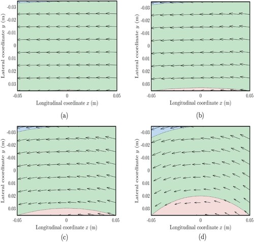
Figure shows the three domains ,
and
for different values of the camber angle
and for
. More specifically, the main green area represents the region
, whilst the red and blue ones are
and
, respectively. It can be seen that larger values of the camber angles cause the two subdomains
and
to be more extended. Of course, for
, the theory reduces to the standard one (see Section 4.3). The black arrows represent the velocity field at each point of the contact patch and are always tangent to circles of arbitrary radius whose centre is located in
. In particular, it can be seen that the arrows located at the right edge of the contact patch (
) point inside, since the bristle are inflowing into the contact area; Analogously, other bristles enter the contact patch from the two lateral edges for
and
, according to the corresponding BCs. Depending on the specific BC which applies in turn, the steady-state tangential deformation of the bristle
will be given by a different expression.
Figure 2. Subdomains ,
and
of the contact patch
(represented by the rectangles) for different values of the camber angle
, 30, 50 and
, respectively. The larger green area corresponds to the domain
, whilst the red and blue one to
and
. The arrows represent the velocity field
and are always tangent to the trajectories of the bristles, which coincide with the characteristics lines given by (Equation41a
(41a)
(41a) ). The length and the width of the contact patch are l = 0.1 and w = 0.07 (m). (a) Domains
,
and
for a camber angle of
. (b) Domains
,
and
for a camber angle of
. (c) Domains
,
and
for a camber angle of
. (d) Domains
,
and
for a camber angle of
.
Hence, we denote with ,
,
the steady-state solutions in the three different domains. We have
(47a)
(47a)
(47b)
(47b)
(47c)
(47c) and
(48a)
(48a)
(48b)
(48b)
(48c)
(48c) where
and
are as follows:
(49a)
(49a)
(49b)
(49b)
(49c)
(49c)
(49d)
(49d)
(49e)
(49e)
(49f)
(49f)
(49g)
(49g)
(49h)
(49h)
(49i)
(49i) in which we have defined
(50)
(50) An interesting result is that the two solutions
and
are continuous at the interface between
and
. Indeed, it is easy to verify that the following relations are satisfied:
(51a)
(51a)
(51b)
(51b)
(51c)
(51c) From a mathematical viewpoint, this structure of this solution is a consequence of the fact
. Conversely, a discontinuity occurs between the regions
and
. This can be explained by looking at the physics underlying the rolling of the tyre. On the one hand, the bristles inflowing in
are the ones which had outflowed from the region
and enter again undeformed at the edge
; on the other hand, the bristles of
which are not transported outside the contact patch keep rolling and their deformation rapidly increases over the travelled distance. We point out, however, that in reality it is unlikely that the contact patch conserves its rectangular shape for large camber angles, whilst there is some evidence in literature that curved geometries can be observed [Citation33,Citation34,Citation61]. We may then conjecture that the third region
disappears; in this case, the deformation would always be a continuous function in space.
4.2. Transient solution
To seek for the transient solution, it is more convenient to express all the dependent variables as a function of the time. In order to do that, we derive Equation (Equation39b(39b)
(39b) ) with respect to the parameter τ, or, equivalently, to the time, and then substitute Equation (Equation39a
(39a)
(39a) ), to get
(52a)
(52a)
(52b)
(52b) Then, integrating (Equation40a
(40a)
(40a) ) and (Equation40b
(40b)
(40b) ) with respect to t and renaming
yields
(53a)
(53a)
(53b)
(53b) where the initial datum (ID)
can be obtained by inverting (Equation52
(52a)
(52a) )
(54a)
(54a)
(54b)
(54b) We note that, in this case, the notion of travelled distance does not apply directly to the quantity s. Indeed,
only represents the main component of the angular speed. However, if
, s may be still interpreted as an averaged travelled distance (note that
is exactly the mean value of the speed field over the contact patch).
Equations (Equation53a(53a)
(53a) ) and (Equation53b
(53b)
(53b) ) represent the general transient solution for the planar vector displacement
, whereas a particular solution can be determined by imposing the IC, i.e. an explicit expression for
. Generally speaking, this IC does not depend on the specific subdomain of
and thus the transient solution is a global one. However, because of the discontinuity in the steady-state solution between the domains
and
, the IC must also be applied separately, i.e. we need
,
and
in
,
and
, respectively. We also need to identify the portion of the space which the transient solution applies to. This investigation can be conducted with respect to each subdomain of
. In order to do this, we can look at (Equation39c
(39c)
(39c) ) and seek for a solution depending on the BC. In particular, from (41b), we deduce that the following conditions must be respectively satisfied for the regions
,
and
:
(55a)
(55a)
(55b)
(55b)
(55c)
(55c) Thus, we can define the following subdomains:
(56a)
(56a)
(56b)
(56b)
(56c)
(56c)
(56d)
(56d)
(56e)
(56e)
(56f)
(56f) so that the general solution for the planar vector displacements reads
(57)
(57) Finally, it is easy to verify that, in each subdomain, the following relations hold for
, Indeed, it is
(58a)
(58a)
(58b)
(58b)
(58c)
(58c) since, after some manipulation, we can find that
,
and
, which implies that the displacements
vanish when evaluated in
because of the boundary prescription. Roughly speaking, this means that the solutions are always continuous at the interface between the steady-state domains and the corresponding transient ones. Furthermore, from the first three of (Equation51
(51a)
(51a) ), we deduce that the curve that makes the transition between the two regimes is continuous at the interface between the subdomains
and
.
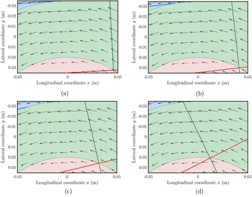
Figure shows the time evolution of the steady-state and transient domains in the contact patch for different values of the nondimensional travelled distance (normalised with respect to the total length) and
. It can be seen that the separation lines which represent the interface between the steady-state and transient solutions of
and
(green and red dashed curves, respectively) are continuous on the circumference
(see Appendix 2). For the region
, it can be also noted that the bristles located in the negative side of the contact patch reach the steady-state conditions faster. This is due to the fact that, for y<0, the main component of the rolling speed and the variable part have are concordant. Conversely, for positive values of y the total longitudinal speed decreases in absolute value because its given by two opposite contributions.
Figure 3. Steady-state and transient domains for each region of for a constant value of the camber angle
and different travelled distances
, 1/8, 1/4 and 1/2. The green, red and blue solid lines represent the interface between the steady-state and transient solution in the domains
,
and
, respectively. More specifically, the steady-state regions correspond to the right portion of the green and red areas for
and
, and to the upper part of the blue domain for
. It can be noted that steady-state conditions are reached in the region
relatively faster (the transient extinguishes in the blue area already for
). The length and the width of the contact patch are l = 0.1 and w = 0.07 (m). (a) Steady-state and transient domains for each region of
for
. (b) Steady-state and transient domains for each region of
for
. (c) Steady-state and transient domains for each region of
for
. (d) Steady-state and transient domains for each region of
for
.
On the other hand, in the domain the bristle inflowing in the contact patch (located at the edge
) are always in steady-state conditions and the transient extinguishes faster in the lower part of the region. This can be explained by considering that the solution is basically given by a wave travelling in space: as the first bristles enter the contact patch, they are propagated towards the trailing edge and steady-state conditions immediately take place, despite the lower values of the speed.
With the same reasoning it is possible to explain what happens in the domain . In this case, the bristles are entering the contact patch from the edge
, and hence the steady-state solution propagates from the upper to the lower part of the blue region. Furthermore, in this case the transient extinguishes even faster, since the rolling speed in the upper side is characterised by a larger longitudinal component in absolute value.
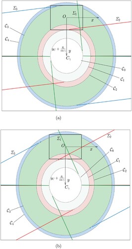
An alternative geometrical interpretation is finally depicted in Figure , where ,
and
are plotted for two different values of the nondimensional travelled distance
and 1/2, respectively. It can be noted that the separation lines between the steady-state and transient subdomains in each region of the contact patch are tangent to the circumferences
,
and
(see Appendix 2 for a more detailed discussion). These circumferences represent the domains for the quantities under the square roots in (Equation49a
(49a)
(49a) ), (Equation49b
(49b)
(49b) ) and (Equation49c
(49c)
(49c) ).
Figure 4. Steady-state and transient domains for each region of for a constant value of the camber angle
and different travelled distances
and 1/2. The functions
and
correspond to the green, red and blue curve, respectively, and represent the interface between the steady-state and blacktransient blacksolution in the domains
,
and
. It can be seen that they rotate tangentially to the circumferences
,
and
. (a) Steady-state and transient subdomains of the contact patch
corresponding to a normalised travelled distance of
. (b) Steady-state and transient subdomains of the contact patch
corresponding to a normalised travelled distance of
.
4.3. Asymptotic analysis
As for the nonlinear case, we need to ascertain that the two-dimensional theory is consistent with the results predicted by the classic one for small values of the camber angle γ and . Starting from the steady-state solution, it is immediate to verify that the two subdomains
and
vanish for γ sufficiently small. Indeed, from Equations (Equation44b
(44b)
(44b) ) and (Equation44c
(44c)
(44c) ), we get
as in the standard brush models. Thus, we only have to analyse the solution
.
In particular, by expanding into Taylor series the square root and the trigonometric functions in (Equation49a(49a)
(49a) ) and neglecting the term y, we get
(59)
(59) The above result also makes allowance for some consideration about the two different areas of
which the steady-state and the transient solution apply to. Indeed, since we have defined
and
, Equation (Equation59
(59)
(59) ) states that, if the camber angle γ is sufficiently small, the two subdomains are separated by the straight line
and the travelled distance regains its original meaning.
For , we expand the trigonometric functions up to the second term and then approximate
to get
(60)
(60) Finally, for
we perform the Taylor expansion of the square root up to the second order yielding
(61)
(61) Note that, with
,
and
defined respectively as in (Equation59
(59)
(59) ), (Equation60
(60)
(60) ) and (Equation61
(61)
(61) ) and performing the change of variables
and
, Equations (Equation47a
(47a)
(47a) ) and (Equation48a
(48a)
(48a) ) reduce exactly to (Equation29a
(29a)
(29a) ).
Now we extend the analysis to the transient solution. We have to find an approximate expression for the ID . Starting from
, we obtain, for small values of γ,
(62)
(62) Analogously, Taylor expansion for
provides
(63)
(63) Combining (Equation53a
(53a)
(53a) ) and (Equation53b
(53b)
(53b) ) with the previous approximate expressions (Equation62
(62)
(62) ) and (Equation63
(63)
(63) ) with the usual change of variables
and
gives again (Equation31a
(31a)
(31a) ) and (Equation31b
(31b)
(31b) ).
5. General theory
Finally, we consider the complete model which accounts for both the coupling between the slips and the spin parameter and for the presence of a two-dimensional velocity field in the contact patch. Since this model combines both the previous ones, we can already infer some properties of the solution. In the first instance, for a rectangular contact patch, we can expect to find the same three regions of the contact patch, namely ,
,
, in which the solution for the deflection of the bristle will be given by a different analytical expression. This analogy with the 2DM is a consequence of the fact that the BCs are only determined by the structure of the vector field (or, equivalently, the characteristic lines of the problem), which is not influenced by the steering ratio
. On the other hand, we may anticipate that each tangential component of the deformation
will depend on both the translational slips
and
, and that slip parameters will multiply nonlinear functions of the spin φ, which are likely to be elementary trigonometric functions.
We start by introducing again the tyre-road contact equations in the following form:
(64a)
(64a)
(64b)
(64b) in which the tangential partial differential operator
has been defined reading
(65)
(65) where the speeds
and
are exactly as in (Equation34
(34a)
(34a) ).
Similarly to [Citation62], we can now look for a general solution in the form
(66a)
(66a)
(66b)
(66b) where
and
can be cleverly assigned to reduce Equation (Equation64
(64a)
(64a) ) to homogeneous form. In particular, the choice
(67a)
(67a)
(67b)
(67b) or, equivalently, in terms of the slip parameters
(68a)
(68a)
(68b)
(68b) turns (Equation64
(64a)
(64a) ) into the following set of PDEs and ODEs:
(69a)
(69a)
(69b)
(69b) together with
(70a)
(70a)
(70b)
(70b) where we have introduced Newton's notation for the time derivative. Note that now
,
and
,
in Equation (Equation66
(66a)
(66a) ) are two independent solutions of (Equation70a
(70a)
(70a) ) and (Equation70b
(70b)
(70b) ).
Now we draw some considerations about the general structure of the solution. Let us start from analysing the first part of the right term of Equation (Equation66(66a)
(66a) ). From (Equation70a
(70a)
(70a) ) and (Equation70b
(70b)
(70b) ), we find
(71a)
(71a)
(71b)
(71b) Furthermore, by means of the method of the characteristics, we are able to solve (Equation69a
(69a)
(69a) ) and (Equation69b
(69b)
(69b) ), which provide
(72a)
(72a)
(72b)
(72b) since the characteristics curve are exactly the same as for the linear two-dimensional case. Thus, we can restate (Equation66
(66a)
(66a) ) as
(73a)
(73a)
(73b)
(73b) where we have denoted with
and
Footnote7. The steady-state solution
can be obtained again by imposing the BCs. In particular, we assume that, with some caution on the invertibility, it is possible to find a parametrisation
Footnote8 for the points
so that
(74a)
(74a)
(74b)
(74b)
(74c)
(74c) By virtue of the (quite rather general) BCs (Equation11
(11)
(11) ), we obtainFootnote9
(75a)
(75a)
(75b)
(75b) and coming back to the original arguments of
and
yields
(76a)
(76a)
(76b)
(76b) where we have introduced
(77a)
(77a)
(77b)
(77b)
(77c)
(77c) Inserting the above expressions (Equation76
(76a)
(76a) ) into (Equation66
(66a)
(66a) ), replacing the time variable t with the travelled distance s, the speeds with the slip parameters, and resorting to elementary trigonometric relations, we obtain the final solution for the steady-state deflections of the bristle
(78a)
(78a)
(78b)
(78b) which are clearly independent of the time variable t (or, equivalently, s). The procedure outlined so far is rather abstract; to give a practical example of how the solutions look like, we can derive an analytical expression in the case of a rectangular contact patch. It is worth pointing out that, for a rectangular shape, the function
reads exactly as in (Equation49
(49a)
(49a) ), depending on the specific BC. In particular, since the BCs and the characteristic curves for the 2DCM are the same as for the 2DM, it is still possible to identify the same regions
,
and
of the contact patch in which the steady-state deflection of the bristle
will be given by a different expression. Moreover, because of the BC prescription, the solutions in the subdomains
and
will be again continuous at the interface
, whilst a discontinuity will occur on
. Summarising, we will have three expressions for
, namely
,
,
, and three expressions for
and
, respectively. More specifically, we can define
(79a)
(79a)
(79b)
(79b)
(79c)
(79c)
(79d)
(79d)
(79e)
(79e)
(79f)
(79f) so that we have the following expressions for the longitudinal and lateral components of the steady-state bristle displacement in the three subdomains
(80a)
(80a)
(80b)
(80b)
(80c)
(80c)
(80d)
(80d)
(80e)
(80e)
(80f)
(80f) On the other hand, to derive the transient solution
, we can proceed analogously as in the previous section, to get
(81a)
(81a)
(81b)
(81b) in which the ID
is exactly as in (Equation54
(54a)
(54a) ). Also in this case, albeit the transient solution is not affected by the partition of the contact patch in a formal way, it must be distinguished amongst a different expression depending on each subdomains of
. Furthermore, we particularly emphasise that the relation
holds between the steady-state and transient solution in each sudomain, i.e. the two solutions are continuous at the interface between their respective domains
and
, which is again represented by the travelling function
. From a physical perspective, this is a direct consequence of the fact that the bristles always enter the contact patch undeformed.
Finally, to prove the consistency of the proposed solutions, we should verify that they are equivalent to the ones obtained in Section 4 for small values of the parameter . The calculations are, however, quite cumbersome, so we do not show the steps. Generally speaking, both the steady-state expressions and the transient one converge to the corresponding formulae found by means of the 2DM by expanding the trigonometric functions into Taylor series up to the first order and then taking the limit for
. By transitivity, it can be also concluded that the 2DCM reduces to the 1DM for sufficiently small values of the coefficient
and camber angle γ.
Remark 5.1
In the preceding analyses, with reference to each model, we assumed . However, if the slip inputs are varied before the transient corresponding to a previous condition is extinguished, the initial conditions are automatically only
. In this case, the analytic solutions obtained by applying the method of the characteristics obviously do not solve the original PDEs, but still represent the only candidate solutions for the weak formulation of the problem. For examples, the transient results shown in [Citation52] for nonzero initial condition clearly represent a weak solution of the 1DM (a strong solution is, indeed, not possible).
6. Model comparison
In this section, we compare the model developed so far against each other and with the classic 1DM. The preceding analyses highlighted different microscopic phenomena which are not captured by the 1DM; macroscopically, these discrepancies may be reflected in a different relation between the generalised forces acting on the tyre and the translational and rotational slips, e.g. the curve.
With reference to the kinematic quantities (basically the slip inputs and the other parameters introduced in 2.1.1), it is firstly necessary to select a minimum set of independent coordinates which fully describe the problem. We can generally assume the existence of a hypersurface Υ so that
(82)
(82) and invoking the IFT we can explicit the variables in interest as a function of the other ones. Perhaps, the most intuitive choice would be to choose the triad
.
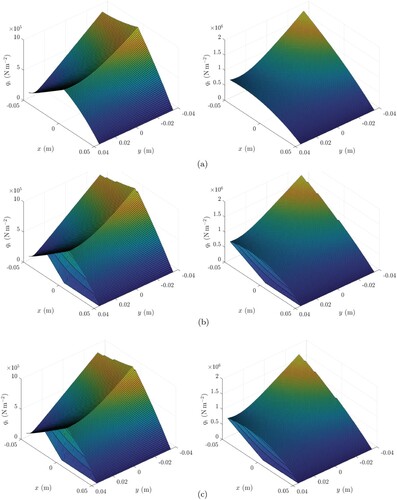
To assess the performance of each model, we carried out different set of simulations in MATLAB environment. For the case of a rectangular contact shape and under the assumption of vanishing sliding (
), the total transient shear stress
acting in the contact patch is shown in Figure for the three different models 1DCM, 2DM and 2DCM and for two values of the normalised travelled distance
and 2, respectively. The pictures refer to the following kinematic parameters:
,
(corresponding to a value of the camber angle of
),
. Generally speaking, it is possible to note an overall agreement in the trend of the predicted shear stress; in particular, the values obtained by employing the 1DCM are slightly higher due to the fact that the bristle displacements are constrained to be zero only at
.
Figure 5. Transient trend of the total shear stress (
,
) predicted by the different models for two values of the normalised travelled distance
(left-hand side subplot) and
(right-hand side subplot). The figures refer to the following values of the kinematic parameters:
,
,
. (a) Total shear stress
predicted using the 1DCM. The left and right-hand side subplots refer to a value of the normalised travelled distance of
and 2, respectively. (b) Total shear stress
predicted using the 2DM. The left and right-hand side subplots refer to a value of the normalised travelled distance of
and 2, respectively. (c) Total shear stress
predicted using the 2DCM. The left and right-hand side subplots refer to a value of the normalised travelled distance of
and 2 respectively.
The assumption of vanishing sliding was then removed to investigate the steady-state problem. Again in the case of a rectangular contact shape, we assumed a parabolic pressure distribution of the type
(83)
(83) where
is the total vertical force acting on the tyre. We also approximated the longitudinal and lateral components of the micro-sliding speed of the bristles in Equation (Equation1b
(1b)
(1b) ) as follows:
(84a)
(84a)
(84b)
(84b) which is a common established approach when dealing with the 1DMFootnote10. Note that the above simplification turns Equation (Equation1b
(1b)
(1b) ) from a PDE into an algebraic relation.
For each model under consideration, the steady-state tyre characteristics were computed numerically starting from the relationsFootnote11
(85)
(85)
(86)
(86)
6.1. Analysis for constant geometric parameters
This analysis was conducted under the assumption of fixed geometric parameters, namely ,
and
. Furthermore, since all the models are supposedly equivalent for sufficiently small values of φ and
, we only investigated the cases in which this two parameters were meant to have a significant impact over the tyre characteristics. Hence, we fixed
and considered the two cases
and
. The first condition describes a scenario in which a heavily cambered tyre (
) tyre is subjected to a low steering speed; the latter, instead, depicts a situation in which the camber angle is limited and the steering speed represents the main component of the spin variable.
The tyre was assumed anisotropic with
and
. The total vertical force on the tyre was set to
N, whilst the static and dynamic friction coefficient were chosen to be
and
. The coordinates of the wheel centre were assumed to be both zero, i.e.
. For the rolling radius we chose
and we assigned the contact patch length and width as l = 0.1 and w = 0.07 m, respectively.
The longitudinal and lateral tyre characteristics are shown in Figure versus the longitudinal slip and for different discrete values of the lateral one
. Regarding the forces acting on the tyre, it is possible to note that high values of the camber angle (
) or the steering speed (
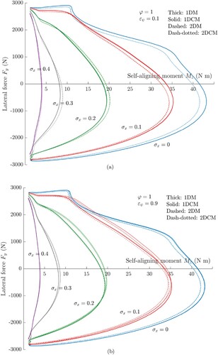
) have a negligible impact on the steady-state values. Variations in the trend of the self-aligning moment
, depicted in Figure , are instead appreciable in both cases; this is probably due to the fact that, for the computation of the moment, the exact distribution of the tangential stresses inside the contact patch plays a crucial role. More specifically, in the first scenario (
), the 2DM and 2DCM predict a similar asymmetric trend for each value of
, whereas the 1DM and 1DCM are not able to capture this phenomenon. Of course, the solution provided by the 2DM aligns quite well with the one found by employing the 2DCM, since the values of the steering ratio are sufficiently small to disregard the coupling between the slips and spin parameter.
Figure 6. Tyre characteristics versus the longitudinal slip for different discrete values of the lateral slip
and steering ratio
. (a) Longitudinal and lateral tyre characteristics versus the longitudinal slip
for different values of the lateral slip
and steering ratio
. (b) Longitudinal and lateral tyre characteristics versus the longitudinal slip
for different values of the lateral slip
and steering ratio
.
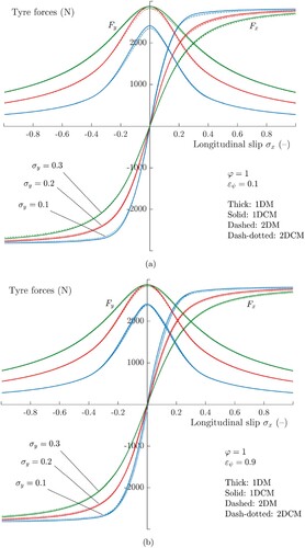
Figure 7. Self-aligning moment versus the longitudinal slip for different discrete values of the lateral slip
and steering ratio
. It can be noted that, for small values of the steering ratio, the 2DM and 2DCM both succeed in estimating the true trend of the self-aligning moment, where the other theories fail; conversely, for larger values of
, the trend is better predicted by the 1DCM and 2DCM. (a) Self-aligning moment versus the longitudinal slip
for different values of the lateral slip
and steering ratio
. (b) Self-aligning moment versus the longitudinal slip
for different values of the lateral slip
and steering ratio
.
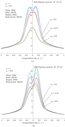
On the contrary, for , the 1DM and 2DM fail in predicting the symmetric trend of the self-aligning moment, whilst the theories for coupled slips and spin both predict a similar trend, with the values foreseen by the 2DCM being slightly lower. From a physical perspective, this can be explained intuitively by considering that the two-dimensional theories prescribe multiple BCs on the edge of the rectangular domain. Since the BCs impose zero deflection of the bristles inflowing the contact patch, this means that they are constrained to adhere to the road in a wider area, and the growth rate in the spatial dimension is more limited.
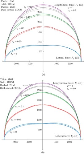
In Figure , the relations are depicted again for different discrete values of
and for the two cases
and 0.9, respectively. This kind of plot is very useful and it is often referred to friction ellipse, since all the point fall within an ellipse which gives the maximum value of the tangential force which can be exerted on the tyre itself. The previous considerations can be extended automatically to the analysis of Figure : for small values of the steering ratio, the 2DM and the 2DCM are totally equivalent and predict the same quantitative trend; on the other hand, as the parameter
increases, the 2DCM aligns more with the 1DCM, since the coupling between the slips and the spin variable becomes preponderant.
Figure 8. Friction ellipses for different discrete values of the lateral slip and steering ratio
. It can be noted that, for small values of the steering ratio, the 2DM and 2DCM both succeed in estimating the true trend of the self-aligning moment, where the other theories fail; conversely, for larger values of
, the trend is better predicted by the 1DCM and 2DCM. (a) Friction ellipse for different values of the lateral slip
and steering ratio
. (b) Friction ellipse for different values of the lateral slip
and steering ratio
.
A last comparison is performed with reference to the diagram in Figure , where the relations are plotted at constant values of the longitudinal slip
. The conclusions which can be inferred are the same as for the previous analyses: the two-dimensional models do not exhibit any discrepancy for
, whilst at larger values of
the mismatch increases and the 1DCM converges to the 2DCM.
Figure 9. diagram for different discrete values of the lateral slip
and steering ratio
. It can be noted that, for small values of the steering ratio, the 2DM and 2DCM both succeed in estimating the true trend of the self-aligning moment, where the other theories fail; conversely, for larger values of
, the trend is better predicted by the 1DCM and 2DCM. (a)
diagram for different values of the lateral slip
and steering ratio
. (b)
diagram for different values of the lateral slip
and steering ratio
.
Generally speaking, the novel models do not predict significant differences from the already-known tyre characteristics from the 1DM. Indeed, the maximum values of the tangential stresses acting in the contact patch is always limited by the available friction; if the same pressure distribution is assumed for all the models, and the structural and geometrical parameters are kept constant, it is reasonable to conjecture that the overall result would not change meaningfully.
6.2. Analysis for varying geometric parameters
High-cambered tyres are expected to undergo significant variations in the geometrical parameters. More specifically, a simple approximation which can be used to model the rolling radius as a function of the camber angle is , where
is the deformed radius of the tyre due to a pure vertical load. Accordingly, the lateral coordinate of the wheel hub centre becomes
, whilst the longitudinal deflection can be assumed to be almost zero. A second theoretical investigation was hence aimed at understanding how these geometrical variations influence the results predicted by the different theories. In particular, to make a fair comparison, we introduced some modifications in the 1DM to account for the term
in the steady-state equations for the deflection of the bristle. In particular, we generalised the steady-state solution for the bristle displacements in (Equation29
(29a)
(29a) ) as
(87a)
(87a)
(87b)
(87b) Simulation results are illustrated in Figure for different values of
and
,
. Generally speaking, even for higher values of
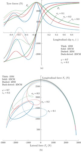
, the coupling between the slips and spin parameters is negligible when the tyre experiences high levels of cambering, and only the 2DM and 2DCM are able to predict substantial discrepancies from the classic theory.
Figure 10. Tyre forces and friction ellipse for an heavily cambered tyre (). When the tyre experiences high level of cambering, the results predicted by the two-dimensional theories exhibit appreciable differences with the ones found by means of the 1DM and 1DCM. (a) Longitudinal and lateral tyre characteristics versus the longitudinal slip
for different values of the lateral slip
and steering ratio
and 0.9, respectively. The tyre rolling radius and the lateral coordinate of the wheel hub centre modelled as a function of the camber angle γ. (b) Friction ellipse for different values of the lateral slip
and steering ratio
. The tyre rolling radius and the lateral coordinate of the wheel hub centre modelled as a function of the camber angle γ.
7. Discussion and conclusion
Brush models are a basic but still effective approach to physical tyre modelling. Indeed, they describe tyre characteristics by means of a minimum set of parameters, which are easy to interpret and to tune, and provide a quite exhaustive understanding of some interesting phenomena concerning the tyre-road interaction. Also, even though brush models are based on some rather simplifying assumptions, they are still able to predict measured forces.
In the present paper, we have extended the brush modelling beyond the standard theory to investigate the effect of the coupling between the slips and a two-dimensional velocity field inside the contact patch. More specifically, we have derived three different models of increasing order of complexity to analyse the contribution of larger spins and camber angles. The first theory concerns the presence of nonlinear relations between the slip parameters and is referred to as one-dimensional model for coupled slips and spin (1DCM). Both for or the steady-state and the transient case, we have shown that, when the spin parameter and the steering ratio, φ and , respectively, are sufficiently large, the deflections of the bristle in the contact patch can be described by nonlinear functions depending on the space variables and the spin itself. The whole formulation is consistent with the classic brush theory, as confirmed by the asymptotic analysis which we have carried out for small values of the steering ratio
and the spin φ.
The second variant which we have developed is the so-called two-dimensional model (2DM), and accounts for large values of the camber angle γ. When the camber is large, indeed, the total speed of a bristle may not be approximated by means of the rolling speed in longitudinal direction, and a more detailed description is needed. In this case, the modelling is further complicated by the fact that multiple BCs must be prescribed, yielding different form of the steady-state solution. The analysis carried out for a rectangular shape shows that it is possible to identify three regions inside the contact patch in which the solution for the vector displacement is provided by a different set of equations. These expressions are highly nonlinear with respect to the space coordinates, but no coupling is predicted between the slip variables. In each domain, the transient solution is again continuous at the transition with the steady-state one. The asymptotic analysis has shown that the novel theory is equivalent to the standard one for small values of camber angles.
Finally, the most general two-dimensional model for coupled slips and spin (2DCM) accounts for both the coupling between the slip parameters and for a two-dimensional velocity field. This model can thus be used when a cambered tyre experiences high steering speeds. The underlying mathematics which the theory is grounded on is, of course, more complicated. However, a procedure to derive the general solution in parametric form has been indicated and some qualitative considerations about its properties have been discussed. Indeed, the characteristics equations are the same as for the linear case, so that some conclusions can be easily extended to the nonlinear theory. In particular, we have shown that three expressions for the steady-state solution can be found in the same subdomains as for the linear model, and that these solutions are independent on the time variable. The explicit formulae provided for the steady-state and transient longitudinal deflections and
, respectively, share some similarities with the solutions found in the case of the two simpler theories developed in this paper. More specifically, the 2DCM theory predicts the coupling between the slip (in turn) and spin parameters and the dependency, for each component of the bristle displacement, on both the translational slip variables.
Limiting the attention to the brush theory, the new models presented in this paper could be useful to study some phenomena which are often neglected by the simplest classic model and deserve to be explored in greater detail. For example, the influence of large camber angles is preponderant during the cornering of motorcycles. Also, recent innovations in the motorsport scenario require extensive investigations about sudden variations in the camber setup. The theory could hence be extended towards real-time applications. Of course, the first step would be experimental validation. Advanced FEM or Multibody tyre models could serve this purpose, or alternatively data collected on a flat track testing machine. However, there are many other directions in which the present work can be potentially expanded. For example, we have already mentioned that the brush models, albeit being effective and particularly pleasing for pedagogical purposes, are probably a very naive approach to physical tyre modelling. As remarked by several authors, in the last years many efforts have been devoted to the development of accurate friction models which may represent a valuable addition to the models developed in the present paper. A natural extension of this work, for example, would be to combine the 2DM with the LuGre formulation to account for a variable velocity field inside the contact patch. It is interesting to note that, for example, an analytical solution to the unsteady-state LuGre model is rarely indicated in literature. The hybridisation with a friction model would also allow to overcome some limiting assumptions introduced in this theoretical analysis. Especially in the context of fast and accurate vehicle dynamics simulation, it is universally acknowledged that static or quasi-static brush models meet annoying difficulties in handling low-speed situations, whereas dynamic models perform much better. Usually, dynamic effects are related to the compliance of the tyre carcass, which has been systematically neglected in the present investigation.
Several strategies proposed in literature could hence be browse. One option could be to conduct a similar study for the stretched-string tyre model [Citation2], which accounts for a distributed deformation of the tyre carcass along the longitudinal direction and has represented the starting point for several derivative models, e.g. the single-point contact point model [Citation2]. However, the assumption of constant deformation in the lateral direction would eventually lead to a paradoxical result, and the incompatibility should be addressed by considering more complex models from advanced beam or membrane theories or by introducing some averaging methods. In this sense, it would be possible to follow, for example, Deur et al. [Citation17] and provide an approximated expression for the function describing the carcass centreline. A recent solution based on the interpolation between the steady-state and transient solution of the tyre-road kinematic equations and called two-regime tyre formulae (TRF) has been developed, amongst the others, by the authors in [Citation52]. This could represent a viable alternative to some stretched-string or LuGre-based enhanced formulations of the classic brush models.
Another possible choice would be to integrate the proposed theories with tyre models developed ad hoc for vehicle dynamics simulations. Whilst taking into account complex road geometries – e.g. uneven roads and soft soil – directly in the brush theory might be prohibitively challenging, it would definitely be beneficial to lean towards hybrid or semi-empirical solutions. To this extent, different algorithms have been developed to determine the position of the (lumped) contact point between the tyre and the road in case of irregular surfaces. These algorithms can be either based on numerical techniques [Citation63] or simplifications of already-existing tyre models [Citation64]. Combining a three-dimensional wheel model with a description of the generalised forces acting on the tyre borrowed from another theory would consist in a quite consolidated approach, and should be taken in consideration.
Nomenclature
Table
Acknowledgments
All the authors gratefully acknowledge the reviewers for the stimulating comments, especially Reviewer III for very insightful considerations which led to a notable improvement of the paper and opened new perspectives for the authors. Luigi Romano particularly acknowledges his friend Milo Viviani for inspiring discussions and suggestions.
Disclosure statement
No potential conflict of interest was reported by the author(s).
Additional information
Funding
Notes
1 In this paper, we use tangential and planar interchangeably.
2 In general, is a three-dimensional position vector
. However, the tangential deflection of a bristle
is always evaluated at z = 0, so we write, with some abuse of notation,
in extended form instead of
. Equivalently, if the travelled distance s is used as independent variable, we write
instead of
.
3 The subscript s stands for sliding.
4 We discriminate between macro parameters, which are independent of the vector position , and micro parameters, which depend on
and are defined locally.
5 Of course, every quantity can be a parameter or a variable depending on the specific problem at hand.
6 The main reason for assuming no sliding is that, in case of finite friction, the IC should be prescribed on an open set which would be unknown a priori. We could also think of defining the IC on the whole interior of the contact patch and then construct the solution to satisfy Equation (Equation1b
(1b)
(1b) ), but this would be formally incorrect.
7 Note that and
are formally identical.
8 The function would correspond to
, but we prefer to use
to lighten the notation.
9 In this paper, the rule for the composition of two functions must be read as
.
10 In general, however, committing this approximation may lead to improper results.
11 We have used the semicolon to distinguish between space coordinates and slip variables. Note that, whilst for the deflection of the bristle the generalised slips can be interpreted as parameters, for the tyre characteristics they represent the main variables. Of course, everything depends on the problem at hand.
References
- Pacejka HB, Bakker E. The magic formula tire model. Int J Vehicle Mech Mobility. 1992;21(1):1–18.
- Pacejka HB. Tire and vehicle dynamics. 3rd ed. Amsterdam: Elsevier/BH; 2012.
- Pacejka HB, Besselink IJM. Magic formula tyre model with transient properties. Vehicle Syst Dyn. 1997;27(sup001):234–249.
- Besselink IJM, Schmeitz AJC, Pacejka HB. An improved magic formula/swift tyre model that can handle inflation pressure changes. Vehicle Syst Dyn. 2010;48(sup1):337–352.
- Farroni F, Giordano D, Russo M, et al. TRT: thermo racing tyre a physical model to predict the tyre temperature distribution. Meccanica. 2014;49:707–723. Available from: https://doi.org/https://doi.org/10.1007/s11012-013-9821-9
- Farroni F. T.R.I.C.K.-Tire/Road interaction characterization & knowledge – a tool for the evaluation of tire and vehicle performances in outdoor test sessions. Mech Syst Signal Process. 2016;72-73:808–831. ISSN 0888-3270. Available from: https://doi.org/https://doi.org/10.1016/j.ymssp.2015.11.019
- Farroni F, Russo M, Sakhnevych A, et al. TRT EVO: advances in real-time thermodynamic tire modeling for vehicle dynamics simulations. Proc IMechE D J Automobile Eng. 2019;233(1):121–135.
- Farroni F, Sakhnevych A, Timpone F. Physical modelling of tire wear for the analysis of the influence of thermal and frictional effects on vehicle performance. Proc Inst Mech Eng L J Mater Design Appl. 2017;231(1-2):151–161.
- Gipser M. FTire – the tire simulation model for all applications related to vehicle dynamics. Vehicle Syst Dyn. 2007;45(S1):139–151. Available from: https://doi.org/https://doi.org/10.1080/00423110801899960
- Gipser M. FTire and puzzling tyre physics: teacher, not student. Vehicle Syst Dyn. 2016;54(4):448–462. Available from: https://doi.org/https://doi.org/10.1080/00423114.2015.1117116
- Gipser M. FTire: a physically based application-oriented tyre model for use with detailed MBS and finite-element suspension models. Vehicle Syst Dyn. 2005;43(sup1):76–91. Available from: https://doi.org/https://doi.org/10.1080/00423110500139940
- Available from: https://www.itwm.fraunhofer.de/en/departments/mf/cdtire.html
- Canudas de Wit C, Olsson H, Astrom KJ, et al. A new model for control of systems with friction. IEEE Trans Automat Contr. 1995;40(3):419–425. Available from: https://doi.org/https://doi.org/10.1109/9.376053
- Sharifzadeh M, Timpone F, Farnam A, et al. Tyre-road adherence conditions estimation for intelligent vehicle safety applications. In: Advances in Italian mechanism science. Cham: Springer; 2017. (Mechanisms and Machine Science; 47). Available from: https://doi.org/https://doi.org/10.1007/978-3-319-48375-7_42
- Sharifzadeh M, Senatore A, Farnam A, et al. A real-time approach to robust identification of tyre–road friction characteristics on mixed- μ roads. Vehicle Syst Dyn. 2019;57(9):1338–1362. Available from: https://doi.org/https://doi.org/10.1080/00423114.2018.1504974
- Canudas-de-Wit C, Tsiotras P, Velenis E, et al. Dynamic friction models for road/tire longitudinal interaction. Vehicle Syst Dyn. 2003;39(3):189–226. Available from: https://doi.org/https://doi.org/10.1076/vesd.39.3.189.14152
- Deur J, Ivanovic V, Troulis M, et al. Extensions of the LuGre tyre friction model related to variable slip speed aong the contact patch length. Vehicle Syst Dyn. 2005;43(supp):508–524. Available from: https://doi.org/https://doi.org/10.1080/00423110500229808
- Deur J, Asgari J, Hrovat D. A 3D brush-type dynamic tire friction model. Vehicle Syst Dyn. 2004;42(3):133–173. Available from: https://doi.org/https://doi.org/10.1080/00423110412331282887
- Velenis E, Tsiotras P, Canudas-de-Wit C, et al. Dynamic tyre friction models for combined longitudinal and lateral vehicle motion. Vehicle Syst Dyn. 2005;43(1):3–29. Available from: https://doi.org/https://doi.org/10.1080/00423110412331290464
- Liang W, Medanic J, Ruhl R. Analytical dynamic tire model. Vehicle Syst Dyn. 2008;46(3):197–227. Available from: https://doi.org/https://doi.org/10.1080/00423110701267466
- Guiggiani M. The science of vehicle dynamics. 2nd ed. Cham: Springer; 2018.
- Bengt JHJ. Vehicle dynamics compendium; 2019. Available from: https://research.chalmers.se/en/publication/513850
- Limebeer DJN, Massaro M. Dynamics and optimal control of road vehicle. Croydon: Oxford University Press; 2018.
- Romano L, Sakhnevych A, Strano S, et al. A novel brush-model with flexible carcass for transient interactions. Meccanica. 2019;54:1663–1679. Available from: https://doi.org/https://doi.org/10.1007/s11012-019-01040-0
- Kalker JJ. Survey of wheel-rail rolling contact theory. Vehicle Syst Dyn. 1997;8(4):317–358. Available from: https://doi.org/https://doi.org/10.1080/00423117908968610
- Kalker JJ, Dekking FM, Vollebregt EAH. Simulation of rough, elastic contact. J Appl Mech. 1997;64:361–368.
- Kalker JJ. Transient rolling contact phenomena. ASLE Trans. 1971;14(3):177–184. Available from: https://doi.org/https://doi.org/10.1080/05698197108983240
- Meymand SZ, Keylin A, Ahmadian M. A survey of wheel-rail contact models for rail vehicles. Vehicle Syst Dyn. 2016;54(3):386–428.
- Kalker JJ. On the rolling contact of two elastic bodies in the presence of dry friction [doctoral thesis]. Delft; 1967.
- Kalker JJ. railway wheel and automotive tyre. Vehicle Syst Dyn. 1979;5(15):255–269.
- Zaazaa KE, Schwab AL. Review of Joost Kalker's wheel-rail contact theories and their implementation in multibody codes. Proceedings of the ASME 2009 International Design Engineering Technical Conferences & Computers and Information in Engineering Conference IDETC/CIE 2009; San Diego, CA, USA; 2009.
- Pacejka HB. The wheel shimmy phenomenon: a theoretical and experimental investigation with particular reference to the non-linear problem [doctoral thesis]. Delft; 1966.
- Higuchi A. Transient response of tyres at large wheel slip and camber [doctoral thesis]. Delft; 1997.
- Higuchi A, Pacejka HB. The relaxation length concept at large wheel slip and camber. Vehicle Syst Dyn. 1997;25(sup001):50–64. Available from: https://doi.org/https://doi.org/10.1080/00423119708969644
- Takács D, Orosz G, Stépán G. Delay effects in shimmy dynamics of wheels with stretched string-like tyres. Eur J Mech – A/Solids. 2009;28(3):516–525.
- Takács D, Stépán G. Micro-shimmy of towed structures in experimentally uncharted unstable parameter domain. Vehicle Syst Dyn. 2012;50(11):1613–1630.
- Takács D, Stépán G, Hogan SJ. Isolated large amplitude periodic motions of towed rigid wheels. Nonlinear Dyn. 2008;52:27–34. Available from: https://doi.org/https://doi.org/10.1007/s11071-007-9253-y
- Takács D, Stépán G. Experiments on quasiperiodic wheel shimmy. ASME J Comput Nonlinear Dyn. 2009;4(3):031007. Available from: https://doi.org/https://doi.org/10.1115/1.3124786
- Takács D, Stépán G. Contact patch memory of tyres leading to lateral vibrations of four-wheeled vehicles. Phil Trans R Soc A. 2013;371:20120427. Available from: https://doi.org/http://doi.org/10.1098/rsta.2012.0427
- Besselink IJM. Shimmy of aircraft main landing gears [doctoral thesis]. Delft; 2000.
- Ran S. Tyre models for shimmy analysis: from linear to nonlinear [doctoral thesis]. Eindhoven; 2016.
- Svendenius J, Wittenmark B. Brush tire model with increased flexibility. European Control Conference; Cambridge, UK; 2015. Available from: https://doi.org/https://dx.doi.org/10.23919/ECC.2003.7085237
- Svendenius J. Tire modelling and friction estimation [dissertation]. Lund; 2007.
- Svendenius J, Gäfvert M, Bruzelius F, et al. Experimental validation of the brush tire model. Tire Sci Technol. 2009;37(2):122–137.
- Nishiara O, Kurishige M. Estimation of road friction coefficient based on the brush model. J Dyn Syst Meas Control. 2011;133(4):9 pages. Available from: https://doi.org/https://dx.doi.org/10.1115/1.4003266
- Albinsson A. Online and offline identification of tyre model parameters [dissertation]. Göteborg; 2018.
- Albinsson A, Bruzelius F, Jacobson B, et al. Design of tyre force excitation for tyre–road friction estimation. Vehicle Syst Dyn. 2017;55(2):208–230. Available from: https://doi.org/https://doi.org/10.1080/00423114.2016.1251598
- van Zanten A, Ruf WD, Lutz A. Measurement and simulation of transient tire forces. SAE Technical Paper 890640; 1989. Available from: https://doi.org/https://doi.org/10.4271/890640
- Mavros G, Rahnejat H, King PD. Transient analysis of tyre friction generation using a brush model with interconnected viscoelastic bristles. Loughborough; Wolfson School of Mechanical and Manufacturing Engineering, Loughborough University; 2004. Available from: https://doi.org/https://doi.org/10.1243/146441905X9908
- Riehm P, Unrau HJ, Gauterin F, et al. 3D brush model to predict longitudinal tyre characteristics. Veh Syst Dyn. 2019;57(1):17–43. Available from: https://doi.org/https://doi.org/10.1080/00423114.2018.1447135
- Chollet H. A 3D model for rubber tyres contact, based on Kalker's methods through the STRIPES model. Veh Syst Dyn. 2012;50(1):133–148. Available from: https://doi.org/https://doi.org/10.1080/00423114.2011.575945
- Romano L, Jacobson F, Bruzelius B. Unsteady-state brush theory. Vehicle Syst Dyn. 2020:1–29. Available from: https://doi.org/https://doi.org/10.1080/00423114.2020.1774625
- Persson BNJ. Theory of rubber friction and contact mechanics. J Chem Phys. 2001;115(8):3840–3861. Available from: https://doi.org/https://doi.org/10.1063/1.1388626
- Persson BNJ, Albohr O, Tartaglino U, et al. On the nature of surface roughness with application to contact mechanics, sealing, rubber friction and adhesion. J Phys Condensed Matter. 2004;17(1):R1–R62.
- Persson BNJ. Contact mechanics for randomly rough surfaces. Surf Sci Rep. 2006;61(4):201–227. Available from: https://doi.org/https://doi.org/10.1016/j.surfrep.2006.04.001
- Xu N, Guo K, Zhang X, et al. An analytical tire model with flexible carcass for combined slips. Math Probl Eng. 2014;2014:Article ID 397538, 9 pages. Available from: https://doi.org/http://dx.doi.org/10.1155/2014/397538
- Kikuuwe R. A brush-type tire model with nonsmooth representation. Math Probl Eng. 2019;2019:Article ID 9747605, 13 pages. Available from: https://doi.org/https://doi.org/10.1155/2019/9747605
- Kalker JJ. Rolling contact phenomena. In: Jacobson B, Kalker JJ, editors. Rolling contact phenomena. Vienna: Springer. (International Centre for Mechanical Sciences (Courses and Lectures), vol. 411).
- Evans LC. Partial differential equations. 2nd ed. Providence, Rhode Island: American Mathematical Society; 2010.
- Ockendon JR, Howison S, Lacey A, et al. Applied partial differential equations. New York: Oxford University Press; 2003.
- Cossalter V, Doria A. The relation between contact patch geometry and the mechanical properties of motorcycle tyres. Vehicle Syst. Dyn. 2005;43(sup1):156–164. Available from: https://doi.org/https://doi.org/10.1080/00423110500141045
- Polyanin AD, Manzhirov AV. Handbook of mathematics for engineers and scientists. Boca Raton (FL): Chapman & Hall/CRC Press; 2007.
- Tengler S, Harlecki A. Determination of the position of the contact point of a tire model with an uneven road surface for purposes pf vehicle dynamicsl analysis. J. Theor Appl Mech. 2017;55(1):3–15.
- Zegelaar PWA. The dynamic response of tyres to brake torque variations and road unevenesses [doctoral thesis]. Delft; 1998. Available from: http://resolver.tudelft.nl/uuid:c623e3fc-b88a-4bec-804a-10bcb7e94124
Appendices
Appendix 1.
Derivation of the steady-state solution for the two-dimensional theory
In this appendix we illustrate the procedure to derive the three expressions for the longitudinal displacement in the domains ,
,
. The same steps can be extended automatically to the lateral problem, so we only consider the longitudinal deflection.
From the first BC in (Equation35(35)
(35) ) we get
(A1)
(A1) where the arguments of
read
(A2a)
(A2a)
(A2b)
(A2b) The above Equation (EquationA2
(A2a)
(A2a) ) can be solved for y and t to obtain
(A3a)
(A3a)
(A3b)
(A3b) Now, some physical considerations are needed to choose the correct sign in the above expressions. As we mentioned before, the characteristics equations for the problem are represented by circumferences of arbitrary radius centred in
on the Oxy plane, which is the point where the wheel axis intercepts the road. This means that, if the camber angle γ is positive, this family of circumferences is centred on the right of the contact patch; conversely, on the left. Since the contact patch includes both points with negative and lateral coordinate, we have to choose the alternative with negative sign when solving for y. From the condition (Equation32a
(32a)
(32a) ), we have to take the solution with the negative sign for
; conversely, if
, recalling the second condition (Equation32b
(32b)
(32b) ), we need to take the solution with the positive sign. Thus, we get
(A4)
(A4) Coming back to the original argument yields
(A5)
(A5) and combining the expression found above with (Equation43a
(43a)
(43a) ) yields the final formula for the steady-state longitudinal deflection
in the region
, which can be restated in compact form by means of (Equation47a
(47a)
(47a) ), together with (Equation46a
(46a)
(46a) ), (Equation49a
(49a)
(49a) ) and (Equation49d
(49d)
(49d) ).
The second BC of (Equation35(35)
(35) ) applies for
. With an analogous procedure as previously, we find
(A6)
(A6) Solving
for x and t gives, respectively
(A7a)
(A7a)
(A7b)
(A7b) where we have to choose the positive solution since the boundary is only defined for
. Substituting into (EquationA6
(A6)
(A6) ) and coming back to the original variables yields for the longitudinal deflection in the second domain
, reading as
as in (Equation47b
(47b)
(47b) ), with
and
defined as in (Equation49b
(49b)
(49b) ) and (Equation49e
(49e)
(49e) ). Finally, in the third domain
, the third BC applies, leading to
(A8)
(A8) As usual, solving
and
provides
(A9a)
(A9a)
(A9b)
(A9b) where we have to choose the negative solution for x (and the positive for the time t), since the BC applies only for
. We obtain the expression for
as in (Equation47c
(47c)
(47c) ), with
and
defined as in (Equation49c
(49c)
(49c) ) and (Equation49f
(49f)
(49f) ), respectively.
Appendix 2.
Determination of the domains for the steady-state solution
The subdomains of the contact patch for which we have the three different solutions must be determined starting from some considerations about the constraint on the space variables. For the solution , we know, from Equation (EquationA7a
(A7a)
(A7a) ), that the following inequality must be verified:
(A10)
(A10) which constitutes the set of points between the two circumferences
(A11a)
(A11a)
(A11b)
(A11b) with
(A12a)
(A12a)
(A12b)
(A12b) where
reads as in (Equation46a
(46a)
(46a) ). Of course, we must only consider the points between the circles which also belong the domain
. Thus, the domain
can be written as
(A13)
(A13) With similar reflections, to find the domain
, we note that from Equation (EquationA9a
(A9a)
(A9a) ) it must necessarily be
(A14)
(A14) which are the points contained by the implicit curves
(A15a)
(A15a)
(A15b)
(A15b) with
(A16a)
(A16a)
(A16b)
(A16b) with
defined as in (Equation46f
(46f)
(46f) ). The domain
is given by
(A17)
(A17) Finally, we can define the region
as the complementary of
to
. We emphasise that the domain
is the only one predicted by the classic brush theory.