Variable wheelbase reference for vehicle with active front and rear-wheel steering

ABSTRACT

Rear-wheel steering has seen new popularity in recent years. Many explanations of rear-wheel steering systems use the concept of a ‘virtual wheel base’ to explain in-phase or out-of-phase steering. This paper introduces a novel reference model that realises this metaphor. A reference model is created where its wheelbase can be changed arbitrarily, making the resulting system intuitive and simpler to design and tune. This augments the properties of the reference model whose signals are used for a feedback control system. The real vehicle tracks these signals using active front and rear-wheel steering. This system can be implemented in a vehicle using steer-by-wire or an autonomous vehicle for control. A MIMO controller is derived and results show that the system operates as intended. Finally, a control law is proposed to change the virtual wheelbase using the road curvature. It is shown that it has advantages over conventional rear-wheel steering control.

KEYWORDS:

• Four-wheel steering
• model reference
• MIMO control
• steer-by-wire
• steering systems
• autonomous vehicles
• variable wheelbase

1. Introduction

The concept of steering the rear wheels of a passenger vehicle has existed since at least 1876 [1]. Its first commercial implementation on passenger vehicles was in 1985 by Nissan on the R31 Skyline for the Japanese market. Its availability has expanded to where almost every major vehicle manufacturer has an option for the technology on at least one of its vehicles. Its proliferation is due in part thanks to the advancement of electric motors with its on-demand power and smaller packaging size, moving beyond the hydraulic actuation and the limitations of pure mechanical actuation it originally used.

Although the means of actuation has matured, the conventional rear-wheel steering (RWS) control methodology has virtually remained the same. At low speeds, a vehicle with RWS uses out-of-phase steering, where the rear wheels steer the opposite of the front wheels. At high speeds, in-phase steering is used, where the rear wheels steer in the same direction as the front wheels. This is typically controlled by a forward velocity dependent mapping.

Academic research has introduced alternative methods of control. Many focus on keeping the body slip angle of the vehicle at zero, or in other words, keeping the centre line of the vehicle body tangential with the turning path [2]. The rationale is that the phase of both the lateral acceleration and yaw rate are the same, giving the driver a better response for handling, in addition to decreasing the phase delay of the lateral acceleration. However, this introduces strong understeer characteristics to the vehicle [3].

Model reference systems are another approach that has been implemented by some researchers. One such system by Abdelfatah, called Yaw Center Control [4], controls the rear wheels of a vehicle by a virtual vehicle whose the front tire angle and the yaw centre can be varied. The yaw centre of the vehicle is the location of the centre of mass. This is shifted forwards or backwards to affect the yaw characteristics of the model reference. The yaw rate is then used as a reference for the rear wheels to steer. Russell has also implemented a model reference based control system [5,6] in a unique application. In her work, the model reference is a vehicle in a low friction condition, and a four-wheel steer-by-wire system is used to track the dynamics on a high friction surface. The control system is composed of a combination of feedforward and state feedback.

Emulating the dynamics of other vehicles has also been done in Lee's work on the Variable Dynamics Testbed Vehicle (VDTV) [7,8]. The goal was to determine how well their VDTV with four-wheel steering can emulate the lateral dynamics on a wide variety of vehicle models, from small to full size. Work done by Akar also shared this goal [9], where the vehicles emulated range from a compact size vehicle up to a bus. The control methodology consisted of feeding back the body slip and yaw rate of the vehicle and the use of sliding mode control.

Implementing rear-wheel steering typically means a compromise in planar dynamics. The lateral acceleration and yaw rate are coupled together because the driver has direct control over the front wheels. Using just the rear wheels to change the vehicle dynamics is restrictive. The future of automobiles are trending to steer-by-wire technology, and eventually, autonomous vehicles where a driver is no longer needed. Nissan has released the first steer-by-wire vehicle with the Infiniti Q50 in 2013, and research has proposed alternative methods of implementing the technology [10]. Autonomous systems will shift the focus on passenger comfort over the handling characteristics and driver feel. Decoupling the yaw and lateral motion of the vehicle can open up design possibilities for engineers. Actuation of the front wheels as well as the rear wheels allows for this decoupling. These actuation abilities can be realised in either a steer-by-wire system or autonomous vehicle system with RWS.

This paper proposes two ideas. The first is a novel model reference where a physical vehicle parameter is transformed into an input to the reference. This allows adjustments of the model reference to be made online, changing the vehicle's properties through a single intuitive input. It is often seen in literature that the control of the rear wheels can be thought of as a vehicle with a changing wheelbase. This virtual wheel base becomes longer when the rear wheels steer in the same direction as the front, and becomes shorter when the rear wheels are steered opposite to the front. This explanation of rear-wheel steering can be implemented as described using the proposed model reference. The wheelbase of the model reference is used to change the characteristics of the vehicle. The reference's new behaviour is tracked by the real vehicle using active front and rear wheels. A MIMO controller is designed which uses feedback to track the reference vehicle's motions. Previous works used signals that are not readily available in commercial vehicles, or needed to integrate observers.

The second idea proposed is a control law for the virtual wheelbase length. This system assumes it can measure the curvature of the road, and a relationship between the current curvature and the virtual wheelbase is developed. This serves as an example for controlling the wheelbase and shows the flexibility of integrating the variable wheelbase into a global scheme.

2. Model reference

The proposed model reference begins with the bicycle model of a car. Its schematic and corresponding bond graph are shown in Figure 1. Its parameters consist of the distance between the C.G. and front axle, a, the distance between the C.G. and the rear axle, b, the mass of the vehicle, m, the moment of inertia about the yaw, $J_z$, and the forward velocity $u_0$. The tire forces are generated through a linear relationship from the slip angle. The slip angles are assumed to be small, and small angle approximations are used.

Figure 1. Planar model of a vehicle with front and rear-wheel steering. (a) Bicycle model of a car. (b) Bond graph of a bicycle model.

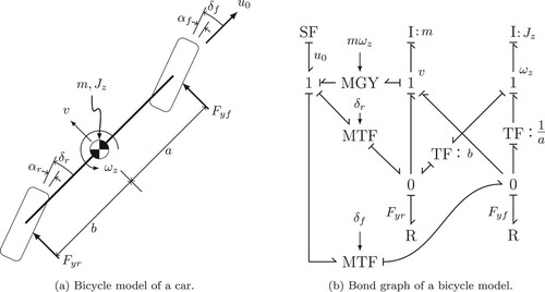
For the model reference, a vehicle with only front steering is considered. Therefore, the rear tire angle ${\delta }_r$ is not used, and can be considered zero for all time. Given this, the equations of motion can be derived as follows: (1) $\begin{array}{rl}{\dot{p}}_v& =-{\displaystyle \frac{C_f+C_r}{m{u}_0}}{p}_v-\frac{1}{J_z}(m{u}_0+{\displaystyle \frac{a{C}_f-b{C}_r}{u_0}})p_{{\omega }_z}+C_f{\delta }_f\end{array}$(1) (2) $\begin{array}{rl}{\dot{p}}_{{\omega }_z}& =-{\displaystyle \frac{a{C}_f-b{C}_r}{m{u}_0}}{p}_v-{\displaystyle \frac{a^2{C}_f+b^2{C}_r}{J_z{u}_0}}{p}_{{\omega }_z}+a{C}_f{\delta }_f\end{array}$(2) where $p_v$ and $p_{{\omega }_z}$ are the lateral momentum and angular momentum of the vehicle, respectively. $C_f$ is the cornering stiffness of the front, while $C_r$ is the cornering stiffness for the rear.

The wheelbase of the model reference, L = a + b, will now be considered an input into the system. The lengths of a and b can both change, so their ratio will be kept constant. Therefore, the lengths can be rewritten as follows: (3) $\begin{array}{rl}a& =\frac{L}{\frac{b}{a}+1}\end{array}$(3) (4) $\begin{array}{rl}b& =\frac{L}{\frac{a}{b}+1}\end{array}$(4) Some intermediate parameters are introduced to simplify the writing: (5) $\begin{array}{rl}\alpha & =\frac{1}{\frac{b}{a}+1}\end{array}$(5) (6) $\begin{array}{rl}\text{β}& =\frac{1}{\frac{a}{b}+1}\end{array}$(6) Therefore, (7) $\begin{array}{rl}a& =\mathrm{\alpha L}\end{array}$(7) (8) $\begin{array}{rl}b& =\text{β}L\end{array}$(8) In this manner, the parameters a and b are now functions of the wheelbase, simplifying the number of variables needed to be changed to just one. The ratio between a and b, $\frac{a}{b}$, is kept constant, such that the centre of gravity effectively stays in place, while the front and rear axles grow and shrink proportionately.

Another consideration is that changing the wheel base would change the mass distribution and therefore the moment of inertia of the vehicle. A good relationship to assume [11] for the moment of inertia which is common among vehicles is (9) $J_z=\mathrm{\kappa mab}$(9) where κ is a dimensionless number, typically $\kappa =1$. However κ is included for finer tuning if desired. Using this relationship allows the moment of inertia to change with the wheelbase. Rewriting this with the equations for the lengths a and b yield the following: (10) $J_z=\mathrm{\kappa m\alpha }\text{β}{L}^2$(10) In reality, however, changing the wheelbase arbitrarily changes the moment of inertia, which takes energy that is not accounted for in the model reference, in addition to many other issues that are not accounted for. This is not a problem since the goal of the model reference is not to create a realistic model of a car that can actually change its wheelbase. The model approximation will be good enough to create outputs for the real vehicle to follow.

Equations (7(7) $\begin{array}{rl}a& =\mathrm{\alpha L}\end{array}$(7) )–(10(10) $J_z=\mathrm{\kappa m\alpha }\text{β}{L}^2$(10) ) can be combined with the equations of motion from Equations (1(1) $\begin{array}{rl}{\dot{p}}_v& =-{\displaystyle \frac{C_f+C_r}{m{u}_0}}{p}_v-\frac{1}{J_z}(m{u}_0+{\displaystyle \frac{a{C}_f-b{C}_r}{u_0}})p_{{\omega }_z}+C_f{\delta }_f\end{array}$(1) ) and (2(2) $\begin{array}{rl}{\dot{p}}_{{\omega }_z}& =-{\displaystyle \frac{a{C}_f-b{C}_r}{m{u}_0}}{p}_v-{\displaystyle \frac{a^2{C}_f+b^2{C}_r}{J_z{u}_0}}{p}_{{\omega }_z}+a{C}_f{\delta }_f\end{array}$(2) ), which yields the following: (11) $\begin{array}{rl}{\dot{p}}_v& =-{\displaystyle \frac{C_f+C_r}{m{u}_0}}{p}_v-\frac{1}{\mathrm{\kappa \alpha }\text{β}}(u_0\frac{1}{L^2}+\frac{\alpha C_f-\text{β}{C}_r}{m{u}_0}\frac{1}{L})p_{{\omega }_z}+C_f{\delta }_f\end{array}$(11) (12) $\begin{array}{rl}{\dot{p}}_{{\omega }_z}& =-{\displaystyle \frac{\alpha C_f-\text{β}{C}_r}{m{u}_0}}{p}_{v}L-{\displaystyle \frac{\frac{\alpha }{\text{β}}{C}_f+\frac{\text{β}}{\alpha }{C}_r}{\mathrm{\kappa m}{u}_0}}{p}_{{\omega }_z}+\alpha C_{f}L{\delta }_f\end{array}$(12) Rewriting the equations of motion in this manner allows for easy modulation of the wheelbase, L, making the system nonlinear. The model reference will now use two inputs: L and ${\delta }_f$. Since the inertia properties change in the derived equations, the system's equations of motions are in terms of its momenta instead of its velocities.

2.1. Wheelbase choice

The choice in wheelbase affects how the vehicle will respond to a driver's inputs. A common parameter for comparing the steering response are the steady state gains. With the derivatives set to zero, the steady-state gains can be derived.

The yaw rate gain and lateral acceleration gain of the standard bicycle model of a car is derived as the following: $\begin{array}{rl}{G}_{{\omega }_z}& =\frac{u_0}{(a+b)+K{u}_0^2}\\ G_{a_y}& =G_{{\omega }_z}{u}_0\end{array}$ where $K=\frac{m(b{C}_r-a{C}_f)}{(a+b)C_f{C}_r}$ In order to investigate the yaw rate gain of the model reference, we will assume L is held constant or changes very slowly. Essentially, the linear system is studied with varying wheelbase length. Therefore, substituting the terms defined previously, the following is derived: $\begin{array}{rl}{G}_{{\omega }_z}& =\frac{u_0}{(\alpha +\text{β})L+K{u}_0^2}\\ G_{a_y}& =G_{{\omega }_z}{u}_0\end{array}$ Note that the understeer coefficient K is invariant to changes in the wheelbase due to the constant a to b ratio. Its clear from the equations that increasing the wheelbase reduces the yaw rate and lateral acceleration gains, while decreasing the wheelbase decreases the gains.

The stability of the linear system can also be explored. The poles of the model reference with various wheelbases are shown in Figure 2. The parameters used can be found in Table 1.

Figure 2. Linear system poles on the s-plane as the wheelbase is modulated over various forward velocities.

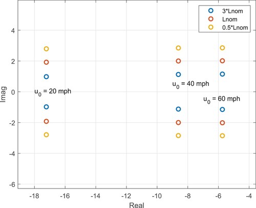
Table 1. Approximate parameters of the D-Class Sedan.

Description	Symbol	Value	Unit
Distance from C.G. to front	a	1.14	m
Distance from C.G. to rear	b	1.64	m
Total mass of vehicle	m	1530	kg
Moment of inertia of vehicle	$J_z$	2732	kg-m${}^2$
Front cornering coefficient	$C_f$	2×68,348	N/rad
Rear cornering coefficient	$C_r$	2×48,578	N/rad

Figure 2 shows the effect of the wheelbase on the poles of the system, where $L_{\mathrm{nom}}$ in the legend is the nominal wheelbase. Increasing the wheelbase lowers the value of the imaginary component of the poles. This also lowers the damping and the natural frequency, but keeps the time constant of the system constant. Increasing the wheelbase has the opposite effect.

3. Plant for controller derivation

The plant used for the design of the controller consists of a bicycle model of a car with added rear-wheel steering, as depicted in Figure 1. The equations of motion are derived as the following: (13) $\left[\begin{array}{c}\dot{v}\\ {\dot{\omega }}_z\end{array}\right]=\left[\begin{array}{cc}-{\displaystyle \frac{C_f+C_r}{m{u}_0}}& -(u_0+{\displaystyle \frac{a{C}_f-b{C}_r}{\mathrm{mu}}})\\ -{\displaystyle \frac{a{C}_f-b{C}_r}{J_z{u}_0}}& -{\displaystyle \frac{a^2{C}_f+b^2{C}_r}{J_z{u}_0}}\end{array}\right]\left[\begin{array}{c}v\\ {\omega }_z\end{array}\right]+\left[\begin{array}{cc}{\displaystyle \frac{C_f}{m}}& {\displaystyle \frac{C_r}{m}}\\ {\displaystyle \frac{a{C}_f}{J_z}}& -{\displaystyle \frac{b{C}_r}{J_z}}\end{array}\right]\left[\begin{array}{c}{\delta }_f\\ {\delta }_r\end{array}\right]$(13) Typical signals easily available in vehicles are the yaw rate and lateral acceleration. If these signals are used for feedback, the transfer functions of the plant are derived and shown below. (14) $\begin{array}{rl}{\displaystyle \frac{{\omega }_z}{{\delta }_f}}\left(s\right)& ={\displaystyle \frac{{\displaystyle \frac{a{C}_f}{J_z}}[s+{\displaystyle \frac{(1+\frac{b}{a})C_r}{m{u}_0}}]}{D\left(s\right)}}\end{array}$(14) (15) $\begin{array}{rl}{\displaystyle \frac{{\omega }_z}{{\delta }_r}}\left(s\right)& =-{\displaystyle \frac{{\displaystyle \frac{b{C}_r}{J_z}}[s+{\displaystyle \frac{(1+\frac{a}{b})C_f}{m{u}_0}}]}{D\left(s\right)}}\end{array}$(15) (16) $\begin{array}{rl}{\displaystyle \frac{a_y}{{\delta }_f}}\left(s\right)& ={\displaystyle \frac{{\displaystyle \frac{C_f}{m}}[s^2+{\displaystyle \frac{b(a+b)C_r}{J_z{u}_0}}s+{\displaystyle \frac{(a+b)C_r}{J_z}}]}{D\left(s\right)}}\end{array}$(16) (17) $\begin{array}{rl}{\displaystyle \frac{a_y}{{\delta }_r}}\left(s\right)& ={\displaystyle \frac{{\displaystyle \frac{C_r}{m}}[s^2+{\displaystyle \frac{a(a+b)C_f}{J_z{u}_0}}s-{\displaystyle \frac{(a+b)C_f}{J_z}}]}{D\left(s\right)}}\end{array}$(17) where (18) $D\left(s\right)=s^2+[{\displaystyle \frac{C_f+C_r}{m{u}_0}}+{\displaystyle \frac{a^2{C}_f+b^2{C}_r}{J_z{u}_0}}]s+{\displaystyle \frac{(a+b{)}^2{C}_f{C}_r}{m{J}_z{u}_0^2}}+{\displaystyle \frac{b{C}_r-a{C}_f}{J_z}}$(18) The transfer function matrix can be arranged as follows: (19) $G_p\left(s\right)=\left[\begin{array}{cc}{\displaystyle \frac{{\omega }_z}{{\delta }_f}}\left(s\right)& {\displaystyle \frac{{\omega }_z}{{\delta }_r}}\left(s\right)\\ {\displaystyle \frac{a_y}{{\delta }_f}}\left(s\right)& {\displaystyle \frac{a_y}{{\delta }_r}}\left(s\right)\end{array}\right]$(19) 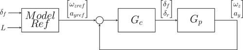The system configuration is shown in Figure 3, where a MIMO controller needs to be generated for the term $G_c$.

Figure 3. System configuration.

From inspection of the plant, it is found that the transfer function matrix loses rank at s = 0, indicating a transmission zero. Decoupling the outputs of the plant at all frequencies is not possible. This is evident from the equation for the lateral acceleration, $a_y=\dot{v}+{\omega }_z\times u_0$. At steady state where the derivatives are zero, the lateral acceleration is dependent on the yaw rate. This is explored further in the controller design.

4. Feedback controller design

The system to be controlled is $2\times 2$, so the MIMO control design is explored using Youla parameterisation [12]. The transmission zero in the plant requires the following interpolation condition to be satisfied in order to avoid unstable pole zero cancellation in the design: $y_z^{H}T\left(z\right)=0$, where z is the zero and $y_z$ is output direction of the zero [13]. The output direction can be derived from a singular value decomposition or a generalised eigenvalue problem.

A technique that can be done with transmission zeros is to move the zero onto a particular output of the system. At steady state, the controller can track a particular signal at low frequencies, while at moderate frequencies, the controller can follow both reference signals. The output direction associated with the zero is $y_z^H=[u_0,-1]$. Therefore shifting the effect of the transmission zero is possible on an individual output channel. Two possible results for the closed-loop transfer function are as follows: (20) $\begin{array}{rl}{T}_{\mathrm{ay}}(s=0)& =\left[\begin{array}{cc}0& {\displaystyle \frac{1}{u_0}}\\ 0& 1\end{array}\right]\end{array}$(20) (21) $\begin{array}{rl}{T}_{\mathrm{wz}}(s=0)& =\left[\begin{array}{cc}1& 0\\ u_0& 0\end{array}\right]\end{array}$(21) Both of these closed-loop transfer function evaluated at the zero location satisfy the given interpolation condition, where lateral acceleration is tracked with $T_{\mathrm{ay}}$ and yaw rate is tracked with $T_{\mathrm{wz}}$. Although both allow for tracking at a particular output channel, they do not behave the same. Choosing to track the yaw rate with $T_{\mathrm{wz}}(s=0)$ yields a system where the largest singular value $\overline{\sigma }=u_0$. This in turn would yield the largest singular value for the sensitivity transfer function matrix $\overline{\sigma }(S_y=0)=u_0$, which is greater than 1 at low frequencies. This choice has very poor properties in the worst output direction. Therefore, choosing to track the lateral acceleration using $T_{\mathrm{ay}}(s=0)$ is pursued.

A closed-loop transfer function matrix is constructed as follows: (22) $T_{\mathrm{ay}}\left(s\right)=\left[\begin{array}{cc}{\displaystyle \frac{s}{(s+{\omega }_1)}}{\displaystyle \frac{{\omega }_2^2}{(s+\frac{2}{\sqrt{2}}{\omega }_{2}s+{\omega }_2^2)}}& {\displaystyle \frac{1}{u_0}}{\displaystyle \frac{{\omega }_1}{(s+{\omega }_1)}}\\ 0& {\displaystyle \frac{{\omega }_2^2}{(s+\frac{2}{\sqrt{2}}{\omega }_{2}s+{\omega }_2^2)}}\end{array}\right]$(22) This satisfies the interpolation condition and produces a stable Y transfer function matrix based on Youla parameterisation (or equivalently Q-parameterisation), where (23) $T_{\mathrm{ay}}=G_{p}Y$(23) Given a stable plant, the feedback control system is stable IFF Y is stable. A controller can then be derived from $G_c=Y(I-G_{p}Y{)}^{-1}$. This particular controller design has two tuning parameters, ${\omega }_1$ and ${\omega }_2$. ${\omega }_2$ is chosen larger than ${\omega }_1$, such that it determines the bandwidth of the system. This is the roll off at higher frequencies for the closed-loop transfer function matrix. A 2nd order Butterworth filter is chosen for both diagonal terms so that the two outputs roll off at the same rate.

${\omega }_1$ is chosen to be small, so that the high pass filter effect happens at lower frequencies for the yaw rate. This also controls the roll off frequency of the coupling between the yaw rate and lateral acceleration signals, required by the interpolation condition.

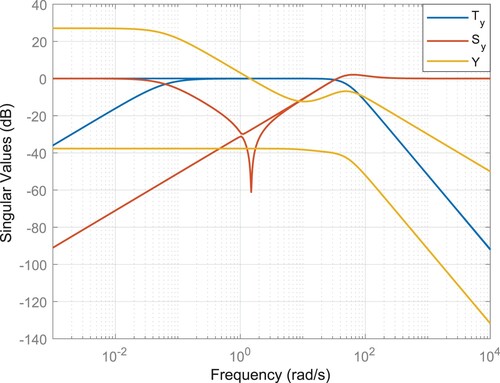
Since real drivers have a steering frequency input of up to $1.5-2\mathrm{Hz}$, we would like the actuator to have a bandwidth of at least double. The frequency roll off is chosen at $8\mathrm{Hz}$, or ${\omega }_2=8\ast 2\pi {\mathrm{rad}\mathrm{s}}^{-1}$. ${\omega }_1$ is chosen experimentally to have good results. The singular value plots of the closed loop, sensitivity, and the actuator are shown in Figure 4.

Figure 4. Singular value plot of the closed-loop response $T_y$, sensitivity $S_y$, and actuator Y.

5. Simulation results

The selected simulations demonstrate how the real vehicle's dynamic properties change with the choice in virtual wheelbase. In order to show the advantages of the proposed system, the simulations will include a conventional RWS implementation. Conventional RWS uses a lookup table which outputs a ratio of rear-wheel steer angle to front-wheel steer angle. This ratio is tabulated according to the forward speed of the vehicle. The conventional system is labelled as ‘Conv’ in the plots. In addition, the nominal vehicle is included which contains no RWS algorithms. This is labelled as ‘Nom’ in the plots.

The control system is applied to a vehicle model from CarSim, a high fidelity vehicle simulation software. This will be the plant $G_p$ depicted in Figure 3. The yaw rate and the lateral acceleration outputs from CarSim are integrated into Matlab/Simulink for use in the MIMO controller. The vehicle used for the simulations is a D-class Sedan. Some approximate parameters of the vehicle are provided in Table 1.

5.1. Open loop with fixed wheelbase length

The simulations presented in this section use the proposed system with the wheelbase length fixed at two lengths. The first is a length three times longer than the nominal wheelbase, can be thought of as a limousine. This is labelled as ‘Long’ in the plots. The second is shortened to half the length of the nominal. This is labelled as ‘Short’ in the plots.

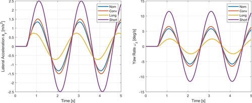
The first simulation set uses a sinusoidal input at the steering wheel after half a second. An amplitude of ${30}^{\circ }$ and a frequency of $0.5\mathrm{Hz}$ is used for a constant forward speed of $48{\mathrm{km}\mathrm{h}}^{-1}$.

The results in Figure 5 show that when the wheel base is made longer, the yaw rate and lateral acceleration are reduced in amplitude. This is expected as the moment of inertia is made larger, making the vehicle less agile and harder to turn. This could hypothetically be used during straight line driving, where the handling and ride could feel more stable and smooth. On the other hand, shortening the wheelbase made the vehicle more agile, with a larger amplitude in the lateral acceleration and yaw rate. This choice would conceivably be better on winding roads that need a faster response and handling. If used in straight line driving, it could make the car feel fidgety evidenced by the high amplitude motion outputs.

Figure 5. Lateral acceleration and yaw rate response to a sinusoidal input at $48{\mathrm{km}\mathrm{h}}^{-1}$.

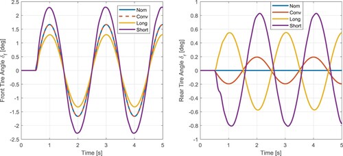
The actuation in the tires is shown in Figure 6. The front tire angles for each set up are the same in phase but differ in amplitude. The short wheelbase reference uses the largest amount of front tire steer. However, the plots of the rear tire angles show the largest differences between the systems. The longer wheelbase has the rear tire angle in phase with the front. The shorter wheelbase is out of phase with the front. This matches the ‘virtual wheelbase’ explanation of rear-wheel steering, and the results match expectations. The tire angle magnitudes are all reasonable. Finally, the conventional algorithm uses out of phase steering. This is because the crossover point from out-of-phase steering to in-phase steering is set up to be at $60{\mathrm{km}\mathrm{h}}^{-1}$. An important concept to note is that the rear tires do not have perfectly aligning zero-crossover points. Although in-phase steering and out-of-phase steering can be seen, the rear tires are not steered according to the front tires for the virtual wheelbase system. They are responding in the manner necessary to track the yaw rate and lateral acceleration that the model reference demands. This is an important distinction between the proposed algorithm and the conventional RWS.

Figure 6. Front and rear tire angles for a sinusoidal input at $48{\mathrm{km}\mathrm{h}}^{-1}$.

The second simulation set also uses a sinusoidal input. An amplitude of ${15}^{\circ }$ and a frequency of $0.2\mathrm{Hz}$ is used for a constant forward speed of $95{\mathrm{km}\mathrm{h}}^{-1}$. These simulations demonstrate the conventional RWS set up steering in-phase with the front for comparison with the proposed algorithm.

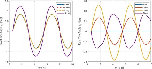
The results in Figures 7 and 8 show similar trends to the first simulation set at $48{\mathrm{km}\mathrm{h}}^{-1}$. The long wheelbase model reference and the conventional system behave similarly with their tire angles, as expected.

Figure 7. Lateral acceleration and yaw rate response to a sinusoidal input at $95{\mathrm{km}\mathrm{h}}^{-1}$.

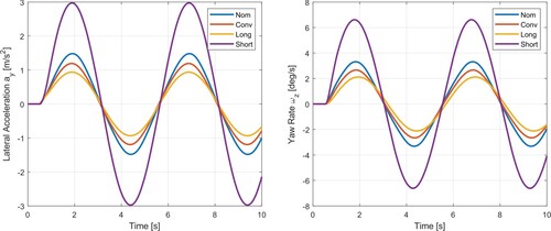
Figure 8. Front and rear tire angles for a sinusoidal input at $95{\mathrm{km}\mathrm{h}}^{-1}$.

Some of the driving cases discussed require a driver to close the loop between the steering input and the path. The next sections demonstrate the systems with a driver model.

5.2. Closed-loop with fixed wheelbase length

The simulations presented integrate a driver model from CarSim to follow a predetermined path. The driver model's steering wheel decision is now exported from CarSim for use in the Matlab/Simulink environment. The driver model's steering wheel input is stepped down through a steering wheel angle to tire angle ratio, and used as the input to the model reference.

A lane change is simulated at $95{\mathrm{km}\mathrm{h}}^{-1}$. The path is a line that shifts over 4 m over a longitudinal distance of 75 m. The driver model's inputs are shown in Figure 9. As expected from the open-loop simulations, for the long wheelbase reference to turn enough, the steering wheel will have to be greater than the other systems. Conversely, the short wheelbase reference needs to steer less.

Figure 9. Steering wheel angle of a lane change at $95{\mathrm{km}\mathrm{h}}^{-1}$.

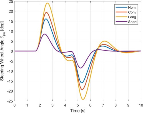
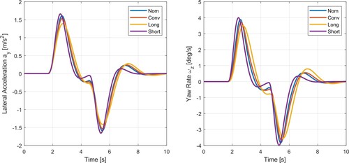
Figure 10 shows that both the lateral acceleration and yaw rates of the longer wheelbase reference are lower in amplitude, and respond slightly slower. The conventional system does trend in the same manner, since the high speed uses in-phase steering. The shortened wheelbase vehicle responds the fastest.

Figure 10. Lateral acceleration and yaw rate response of a lane change at $95{\mathrm{km}\mathrm{h}}^{-1}$.

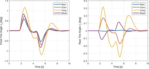
Finally, the tire angles are shown in Figure 11. The tire angles are reasonable and not excessive.

Figure 11. Front and rear tire angles of a lane change at $95{\mathrm{km}\mathrm{h}}^{-1}$.

The proposed algorithm still requires the wheelbase to be set. As discussed, having the vehicle feel longer during straight driving and shorter in curvy roads could have benefits for handling. As a preliminary study into this idea, a control law for the wheelbase length is proposed in the next section.

5.3. Closed-loop test with dynamic wheelbase

So far the simulations shown use a constant wheelbase where various lengths are compared. The vehicle will now track the yaw rate and lateral acceleration signals while the wheelbase of the model reference varies.

One idea of implementation is for an autonomous vehicle, where if a vehicle has knowledge of the path ahead, the model reference can adjust in order to best negotiate. In traditional RWS control where only the forward velocity is fed back, the system has no knowledge of what the intentions of the driver are. A highway off ramp and a lane change are treated the same. However, knowledge of the curvature of the road is helpful in negotiating a turn, because the vehicle properties can change to reflect the upcoming driving scenario. If a vehicle wants to simply change lanes on a straight stretch of highway, having the vehicle behave like it has a longer wheelbase could reduce the amount of yaw rate. The car would simply drift to the next lane without having to yaw the vehicle very much. If the vehicle is negotiating a series of winding curves, a shorter wheelbase would allow for more yaw rate and allow the vehicle to handle better.

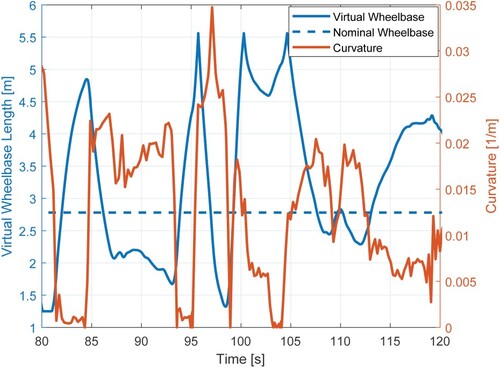
In the following simulation, a course is negotiated by a driver model in CarSim which is made up of winding turns and curves. Therefore, a simple proposal is made. Assuming that the autonomous vehicle can generate the curvature of the road, the wheelbase will be a function of the curvature. When the path is straight, the wheelbase is long. When the curvature increases, the wheelbase should begin to shrink. Therefore, the following control law is proposed: (24) $L=L_{max}-k|\rho |$(24) where ρ is the curvature relative to the vehicle, k is some choice in slope with units of m${}^2$, and $L_{max}$ is the longest wheelbase desired while the road is at a straight path. When the path begins to curve, the wheelbase shrinks. The proposed control law linearly reduces the wheelbase as the curvature increases. More complicated choices can be implemented as well. A saturation operator is added to limit the wheelbase so it does not become too small.

In the simulation, the driver model can also accelerate and decelerate, limited to a total acceleration of $5{\mathrm{m}\mathrm{s}}^{-2}$. The vehicle's speed varies from 40 to $120{\mathrm{km}\mathrm{h}}^{-1}$ under these limitations. However, the model reference is based on a planar model with constant forward speed. In order to have more realistic lateral acceleration reference signals, the vehicle's actual speed is fed back to the model reference under the assumption that the vehicle's forward change in speed is not extreme.

The results show that the driver model successfully navigated the course with the varying wheelbase system. Figure 12 shows a snapshot of the lateral acceleration and yaw rate. Included for comparison are the conventional RWS system and the nominal vehicle without RWS. A location to note on the plot is at around 96 s, where the variable wheelbase has higher peaks in the signal outputs. This is due to the virtual wheelbase being long at that point in time. The driver model is attempting to stay on a generated path for the course, so it steers aggressively to track the path. An idea for remedying this is using the curvature of the path ahead of the vehicle instead of the instantaneous path at the vehicle. Regardless, the signals show smoother movement in the motion outputs.

Figure 12. Yaw rate and lateral acceleration signals on a course in CarSim.

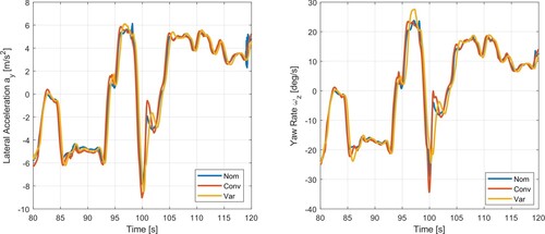
Figure 13 shows the actuation of the front and rear tires. The rear tires do not exceed $5^{\circ }$ in the snapshot of the simulation, which is reasonable.

Figure 13. Front and rear tire angles of the vehicle on a course in CarSim.

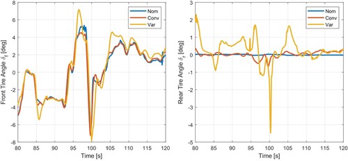
Figure 14 demonstrates the steering wheel motion for navigating the course. The larger steering angles of the variable wheelbase system coincide with a longer wheelbase, shown in Figure 15. Figure 15 shows the curvature and reference wheelbase chosen by Equation (24(24) $L=L_{max}-k|\rho |$(24) ). The wheelbase change uses a smoothing filter in order to avoid abrupt changes. The wheelbase control proposal is not sophisticated by any means, but accomplishes the goal of demonstrating this proof of concept.

Figure 14. Steering wheel angle on a course in CarSim.

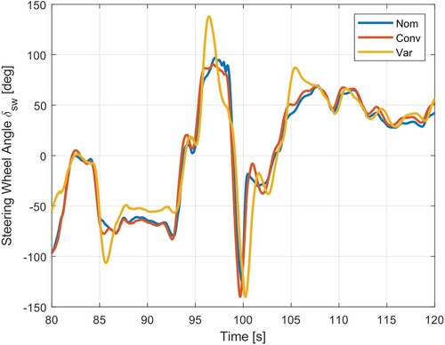
Figure 15. Model reference wheelbase and curvature of the road on a course in CarSim.

6. Conclusion

To conclude, a novel proposal for controlling the front and rear wheels has been described and demonstrated. The system described allows a vehicle with active front and rear wheels to handle like a long limousine, or a small nimble car. The model reference is set up such that the only parameter needed to change is the wheelbase length, which is intuitive to control. In the open-loop simulations, it was demonstrated that the longer wheelbase outputs less yaw rate and lateral acceleration, as expected with a real vehicle comparison. A shorter wheelbase was just the opposite.

Further research can investigate adding fidelity to the model reference. For manoeuvring at higher lateral accelerations, the model reference needs tire forces that can saturate in order to avoid unrealistic lateral acceleration references, which can destabilise the system. In addition, the two degree-of-freedom system can be extended to a three degree-of-freedom system, allowing for longitudinal acceleration which was not done in this paper. This would also be helpful for extreme handling situations. Additionally, passenger comfort and handling needs to be properly investigated though quality evaluations. This can be done through virtual simulators.

The use of feedback in the system indicates that there can be robustness to disturbances, such as wind gusts. Further research can investigate the robustness of the control system due to uncertainties of the vehicle parameters, sensor noise, and disturbances.

Furthermore, a simple control proposal is used to control the wheelbase. A proof of concept shows successful tracking of reference signals by the controller while the wheelbase changes dynamically during simulation. Further research can investigate a more sophisticated choice in controlling the wheelbase of the model reference.

Acknowledgements

The authors would like to thank Hyundai Motor Company for their support.

Disclosure statement

No potential conflict of interest was reported by the author(s).

References

- Gilmore CP. What's news. Popular Sci. 1986 Feb;228(2):59.
- Sano S, Furukawa Y, Shiraishi S. Four wheel steering system with rear wheel steer angle controlled as a function of steering wheel angle. SAE Technical Paper 860625; 1986.
- Shibahata Y, Irie N, Itoh H, et al. The development of an experimental four-wheel-steering vehicle. SAE Technical Paper 860623; 1986.
- Abdelfatah MM. Yaw center control of a vehicle using rear wheel steering. In: Klomp M, Bruzelius F, Nielsen J, et al. editors. Advances in dynamics of vehicles on roads and tracks. IAVSD. Cham: Springer; 2019.
- Russell HEB, Gerdes JC. Low friction emulation of lateral vehicle dynamics using four-wheel steer-by-wire. 2014 American Control Conference; Portland, OR; 2014. p. 3924–3929.
- Russell HEB, Gerdes JC. Design of variable vehicle handling characteristics using four-wheel steer-by-wire. IEEE Trans Control Syst Technol. 2016 Sep;24(5):1259–1240.
- Lee A. Emulating the lateral dynamics of a range of vehicles using a four-wheel-steering vehicle. SAE Technical Paper 950304; 1995.
- Lee A. Matching vehicle responses using the model-following control method. SAE Technical Paper 970561; 1997.
- Akar M, Kalkkuhl JC. Lateral dynamics emulation via a four-wheel steering vehicle. Vehicle Syst Dyn. 2008;46(9):803–829.
- Arasteh E. Steering system with a differential for additive active steering and autonomous operation [master's thesis]. Davis: University of California, Davis; 2018.
- MacInnis D, Cliff W, Ising K. A comparison of moment of inertia estimation techniques for vehicle dynamics simulation. SAE Technical Paper 970951; 1997.
- Assadian F. MAE 272 theory and design of control systems. Class lecture. Davis: University of California; 2015.
- Skogestad S, Postlethwaite I. Multivariable feedback control analysis and design. 2nd ed. Chichester: Wiley; 2005.