Energy-optimal overtaking manoeuvres of Formula-E cars

Abstract

Overtaking in motorsport races is a crucial action in order to gain a higher position during a race. In Formula-E, it not only requires precisely performed overtaking manoeuvres but also requires appropriate energy management which is also a crucial element in race strategy due to the limited total amount of energy on board. This study proposes the use of optimal control techniques for feasibility and energy management analysis for such a complex problem. The analysis involves two cars on a track and the goal is to find the optimal overtaking strategy under various scenarios. The results demonstrate that overtaking can be infeasible despite that there is a potential speed advantage over the target car. An overtaking manoeuvre can be executed efficiently by using higher propulsion power. When an overtaking is feasible, the energy-optimal overtaking position varies according to different initial conditions.

KEYWORDS:

• Energy management
• Formula E
• overtaking manoeuvres
• optimal control

1. Introduction

In motorsport races, overtaking is one of the most tricky but exciting and breathtaking manoeuvres. In most cases, overtaking is an essential action to gain higher positions on the track, which leads to higher rewards. Overtaking may happen both in the pitlane (due to different refuelling or tyre change strategies) or on the track. The former one requires more from the race strategy management to create a chance of undercut or overcut on a multi-lap level. In contrast, the latter one requires more from the driver and vehicle. This means that either the driver needs to be adventurous enough to make a bold move or the race car itself must have some net advantages (e.g. power and handling) over the other competitors. A successful overtake requires good trajectory planning with execution and proper management of the resource either vehicular (e.g. power energy) or environmental (e.g. slipstreaming from another car).

In the literature, the studies for overtaking manoeuvres focused on developing controllers in real-time to complete the manoeuvre. These fall into two main categories, overtaking by lane changing for road car applications and controller development for race car applications.

The number of researches for race car overtakes is very limited and they are mainly completed in simulation game environments, such as The Open Racing Car Simulator (TORCS). Developing control algorithms in racing games has been a topic because of the convenience of the simulation environment [1–3]. However, the commonly overtaking strategy in games is relatively simple which is sensing opponent cars as static obstacles and finding a clear path through [4]. For novel overtaking techniques, Onieva [5] added a decision layer using fuzzy logic to the basic underlying control layer aiming to overtake opponents with blocking strategies. The limit of this study is that the odds of successful overtaking are under 50% and the experiments were completed only on long straights. Loiacono [6] proposed the use of machine learning techniques to tackle the challenge of overtaking. The study focused on two scenarios: (1) long straights and large corners and (2) tight bends. The tests were conducted against non-player character (NPC) drivers in the game. The utility of Q-learning is proved in developing overtake techniques of slipstreaming and late braking for the two scenarios. Similarly, Huang [7] also adopted Q-learning for overtaking studies which were experimented with in more complicated tracks and proved to be able to learn both overtaking and blocking skills. Although these studies showed that the overtaking manoeuvres can be solved, the experiments in these cases have some common limits. (1) The test tracks were relatively simple. (2) The level of NPCs was poor which created big chances of being overtaken by the actor vehicle. (3) The fuzzy architecture used in [5] is composed of general if–then rules which were not able to give a precise analysis of overtaking possibilities. (4) Q-leaning technique has its natural stochastic feature which makes it very difficult to generate an optimal overtaking solution.

The majority of overtaking research mainly focus on autonomous road vehicles. An overtaking manoeuvre can typically be divided into sub-manoeuvres as: (1) moving to another lane; (2) passing the target vehicle; and (3) merging back to the normal lane. The methods used for trajectory planning for these manoeuvres fall into three main categories. (1) Potential field algorithms assign potential values to the path fields ahead to describe the safety levels along the path [8]. The quality of generated path depends heavily on the potential value assignment which is based on knowledge of the environment. And the safety is possibly compromised due to the lack of accounting for vehicle kinematics in high-speed scenarios [9,10]. (2) Tree search techniques such as rapidly exploring random tree (RRT) [11] are also popular for path planning. Vehicle constraints can be incorporated into the calculation. But such decomposition algorithms might generate sharp path curvature changes due to discontinuity in the tree search and result in discomfort for passengers [12]. And the size of the tree would significantly affect the computational cost of the algorithms [11]. (3) Model predictive control (MPC) methods which previously have been used widely for path tracking controllers, recently have been used in research for path planning. And a sequence of controls can be solved simultaneously with the path [13,14]. (4) Optimal control-based methods target to minimise a cost function under a number of constraints. In such methods, various factors can be accounted for (e.g. vehicle limit, environment constraints, driver comforts) [15,16]. While the latter two categories are promising robust methods for path planning due to their ability to incorporate multiple dynamic features and constraints, for the faster computational speed required by real-time applications, the models used to formulate these problems are still mostly simplified (e.g. point mass vehicle model, bicycle model with no non-linear features). A generated path might not be feasible for path tracking controllers which might lead to safety issues [17].

In high-level motorsport races, optimisation of overtaking manoeuvres is a complex problem to analyse in which several factors cannot be neglected. First, overtaking relies largely on utilising the full envelope of the race car performance. Therefore, complex system models are needed to describe the system dynamics in the calculation. Second, overtaking is always an expensive manoeuvre that comes with costs in resources such as energy, fuel or tyre life. It also brings penalties such as heat generation or tyre degradation. In races with restrictions on resources (e.g. Formula one tyre usage [18], Formula E energy consumption [19]), aggressive overtaking might raise resource crisis in later laps. This further raises an overtaking problem into a management problem with a very long optimisation horizon (track length, lap level). In this case, real-time MPC algorithms are no longer suitable because their relatively shorter prediction horizons will easily yield sub-optimal solutions and it is hard to formulate a long-horizon management problem into sub-problems. An overtaking manoeuvre needs to be executed in a way as efficient as possible so that being re-overtaken later due to saving the over-consumed resource can be evitable. Third, highly professional drivers and teams rarely make mistakes that offer their opponents easy opportunities to overtake. The solution for overtaking manoeuvres has to be optimal to guarantee a gain in the position even given a very small probability of success.

In recent motorsport-related research, optimal control techniques are widely used for single-car optimal minimal time manoeuvre (MTM) and lap time simulation studies. Giacomo et al. [20,21] proposed to use the optimal control technique to generate a track in 2D (i.e. a plane track) and 3D (i.e. a spatial ribbon) spaces. The problem was formulated to control the curvatures, rotations, and track widths to minimise the sum of the integral error to the surveyed GPS coordinates and the change rate of the controls under the closure constraints of a closed track. The majority of the minimal time relating research use 2D tracks to simplify the problem. Tremlett et al. [22] studied the optimal limited-slip differential (LSD) bias profile on U-shape turn with different road-tyre frictions. Similarly in [20], LSD bias was studied on a closed track but was proposed as a constant vehicle parameter to be optimised simultaneously as the optimal control problem (OCP) being solved. In [23], a thermodynamic model and tyre wear model were introduced into the problem. The influence of tyre temperature on performance was studied and an optimal tyre warming up strategy was investigated. It also shows that vehicle setups can be optimised to minimise tyre wear. The powertrain has been another category of related research. Limebeer et al. [24] studied the optimal control for the formula one hybrid powertrain. The result demonstrated that with proper management of the new hybrid system, one-third of the fuel can be saved compared to the earlier pure internal combustion powertrain. Soren et al. [25] fixed the driving path in the problem to improve the computational efficiency for the hybrid powertrain management. They also proposed a real-time implementable method to control the powertrain by using analytic derivations. Because full-electric motorsport has become popular, Herrmann et al. [26] studied the optimal energy management of full-electric autonomous race cars. Liu et al. [27] studied the optimal energy and thermal management strategy for Formula-E cars for single-lap and multi-lap scenarios [28]. Lifting and coasting techniques were developed to save energy and the effect of energy consumption restriction on race lines and lap times was demonstrated. In more complex studies, the vehicle model is improved to be used on a 3D ribbon track [20,28] with banking and elevation features. Masouleh et al. [29] introduced a multilink suspension into the vehicle modelling and the aero-suspension interaction feature was incorporated. The vehicle setups and aerodynamics features were optimised to fully improve the aerodynamic influence on the car to minimise the lap time. Dal Bianco et al. [30] compared the computational performance of direct and indirect methods for OCPs because the computational time for such minimal lap time is usually long (dozens of minutes).

In this paper, we proposed a novel approach to formulate a lap time simulation, which allows analysis of the performance of a car with the presence of an opponent car. This introduces to the industry a new element in pre-race preparations and enables engineers to analyse the maximum performance that can be extracted with the influence of an opponent car. This further provides engineers a better understanding strategies multi-car scenarios. It also potentially introduces another dimension in race-level strategy development where more complex strategies or even dominant strategies for securing a higher position based on the understanding of overtaking feasibility can be investigated.

Optimal control techniques are used in this study to solve the overtaking problem with complex system dynamics, a large optimisation horizon, and the multiple constraints and components of the cost function. The overtaking manoeuvres combined with the energy management strategy of Formula-E cars are studied. The first section of this paper introduces the background of overtaking in motorsport and previous research about minimal time OCPs and overtaking manoeuvres. In Section 2, the generation of reference trajectories will be demonstrated and overtaking opportunities will be explained. Section 3 presents the formulation of the overtaking OCP. Section 4 includes the optimal solutions of overtaking manoeuvres and essential conditions for a successful overtaking will be discussed. The conclusions will be summarised in Section 5.

2. Reference performance and overtaking opportunities

In this paper, for both reference trajectories and the vehicle being controlled, the curvilinear coordinate system is used to describe the track. The vehicle is described using a 7DOF planar model with longitudinal, lateral, yaw motions with four-wheel rotations. Steering input is applied on the front wheels. Drive and regenerative brake torque are applied on the rear wheels and a mechanical brake applies on the front wheel. An LSD is modelled on the rear axle. Aerodynamics and load transfer effects are also included. We choose not to use higher-fidelity models to include pitch and roll motions in this study because the motions of pitch and roll are more of a priority when a task is more dominated by vehicle dynamics studies. In high-level motorsport (i.e. Formula One and Formula E), the roll and pitch motions themselves have relatively low magnitudes due to the high stiffness of suspensions on these cars. The main reason why these are important is that they have a crucial effect on aerodynamics performance like in Formula One where aerodynamics downforce character is one of the dominant factors thus cannot be overlooked in performance analysis [29]. However, in Formula E, the bodywork used by teams is identical and its design concept is very different from formula one [31] and is of much less concern in downforce generation thus the performance is less aerodynamic dependent or sensitive to pitch and roll motions [32]. The details of the models are presented in Appendix A.

2.1. Reference trajectory and performance

In motorsport races such as Formula One and Formula E, energy whether electric or fuel, is never adequate enough for drivers to flat out through the entire race. It is a limited resource that drivers and engineers have to carefully manage every lap. For example, in a formula E race, ‘energy per lap’ (EPL) which indicates the target energy consumption during a single lap, is a crucial factor. It is commonly way lower than the energy consumption of a flat-out lap during which energy saving is not considered. And exceeding it will potentially lead to a flat battery before the race finishes.

According to [27], the most common way to save energy while maintaining a competitive speed is through lift and costing (LaC) techniques. An example of such a technique is shown in Figure 1.

Figure 1. Speed profiles using different EPLs.

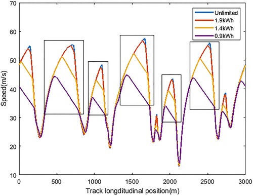
In general, what the driver needs to do is to lift his foot off the acceleration pedal and let the car coast by its momentum with or without a certain amount of regenerative coasting torque. This technique is used when the car reaches a relatively higher speed, normally near the end of a straight before applying the brake. As shown in the figure, this results in a speed disadvantage compared to the unlimited case which is the performance without considering energy saving. Lower EPLs bring larger speed disadvantages.

The track used in this study is the Marrakesh E-Prix track. To analyse overtaking manoeuvres, the trajectories of a reference car, namely the target car is needed. To generate such reference trajectories, a single-car OCP of MTM is formulated with a boundary constraint of EPL and based on the cost function of (1) $J={\int }_{s_0}^{s_t}Sfds,$(1) where $s_0$ and $s_t$ are the initial and terminal length of the track, respectively, $S_f$ representing the reciprocal of the vehicle velocity along the track centreline which is defined in the track model in Appendix A. The energy constraint is added as (2) $g_{bE}={\int }_{s_0}^{s_t}(P\mathrm{\_}power\cdot Sf)ds<E_{epl}$(2) in which $E_{epl}$ is the upper limit of total energy consumption per lap, $P_{power}=P_{drive}+P_{regen}$ is the combination of propulsion and regeneration power given by (3) $\begin{array}{rl}{P}_{drive}& =(T_{drive}+T_{diff\mathrm{\_}r}){\omega }_4+(T_{drive}-T_{diff\mathrm{\_}r}){\omega }_3,\end{array}$(3) (4) $\begin{array}{rl}{P}_{regen}& =(k_r(1-k_b)T_{brake}+T_{dif{f}_r}){\omega }_4+(k_r(1-k_b)T_{brake}-T_{diff\mathrm{\_}r}){\omega }_3\end{array}$(4) in which $k_r$ denotes the portion of regenerative brake in total brake torque, $k_b$ is the brake bias to the front, $T_{drive}$ and $T_{brake}$ are drive torque from the motor brake torque generated by the calliper or the motor regeneration, ${\omega }_3$ and ${\omega }_4$ are the rotational speeds of rear right and left wheels, respectively, $T_{diff\mathrm{\_}r}$ is the LSD torque transferred from the faster-rotating wheel to the slower wheel. It should be noted that $P_{drive}$ is also given an upper limit based on the power mode, which will be explained in the next section. This reference generation procedure of a single-car scenario is thoroughly explained in [27] thus, it is not detailed here. The track layout and example trajectories are shown in Figure 2.

Figure 2. Track layout and trajectory examples: (a) track layout and (b) enlarged block A.

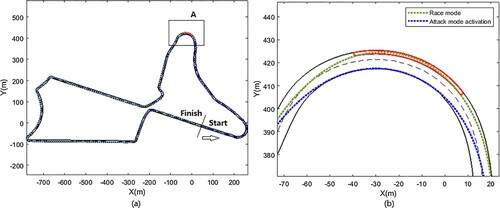
The blockedzone on the upper side of the track in Figure 2(b) is called the activation zone, which is a unique feature in Formula-E races. This will also be explained in the next section. To avoid confusion in the following sections in this paper, the ‘reference car’ will be referred to as the target car and the car attempting to overtake will be called the ‘actor car’.

2.2. Overtaking opportunities

A successful overtaking is a result of the actor car’s speed advantage over the target car. In Formula-E, the speed advantage comes from two main causes (neglecting human errors and car failure). The first one is from different EPL targets between the actor and the target car. As is previously shown in Figure 1, when the actor car is given a higher EPL, it is allowed to achieve higher speed with less LaC to execute. This speed advantage will lead to potential overtaking opportunities when the target car is doing LaC and the actor car is allowed to further accelerate. The second way to create speed advantages is to use higher propulsion power. This is a unique feature of Formula-E races. The technical regulation [19] of FE states that during a race, the maximum propulsion power is limited to 200 kW in Race Mode settings. Beyond that, teams are given options of activating ‘attack mode’ for a certain amount of time (typically around two laps) which gives an extra power of 50 kW using this mode. To activate the attack mode, cars need to drive through the activation zone which is normally deviated from the normal race line. On the Marrakesh E-Prix track, it is the red zone shown in Figure 2(b). After driving through the activation zone, the power limit is raised to 250 kW allowing the actor car to chase the target car in a more aggressive way. Such lap will be referred to as ‘activation lap’ later in this paper. In the second lap after activating the attack mode, the car does not have to drive through the activation zone again to keep using the 250 kW attack mode. It also should be noted that when the target car needs to drive through the activation zone, it clears out the normal race line, which also becomes a potential overtaking opportunity. This will be shown in the result section.

2.3. Collision constraint

Speed advantages do not necessarily lead to a successful overtaking due to the existence of the target car on the track which changes the trajectory space. Apart from the track bounds, the actor trajectory must not cause a collision with the target car. In the application of autonomous vehicles trajectory planning, multi-vehicle collision avoidance is usually treated as a soft constraint of which the collision-avoidance cost is minimised each step in the optimisation horizon [33]. In motorsport, lap time or energy is the sole cost to minimise. Adding a collision-avoidance cost in the step cost function will compromise the optimality of the solution of either time or energy. Therefore, in this study, the collision constraint will be treated as a hard constraint.

Two main assumptions are accounted for when formulating this constraint. Firstly, the target car trajectory does not change inside every single case. This mainly accounts for the fact in real life motorsport that no driver would give up the optimal line to initiatively avoid collision when an opponent is trying to overtake. This is different from cooperative autonomous trajectory planning [34] where the trajectories of each car are optimised simultaneously and cooperatively to avoid the collision. The second assumption is that the actor car is allowed to overlap the target car trajectory once it gains the longitudinal position advantage greater than zero. The main reason for this ‘collision neglecting’ assumption is to consider the priority on the track. Once the actor passes the abreast position with the target car, it is given the priority of manoeuvre and the overtaken target car becomes responsible for collision avoidance. This is usually referred to as ‘blocking’ or ‘defending’ position in motorsport. Based on these two assumptions, the collision constraint used in this study is illustrated in Figure 3.

Figure 3. Collision exclusive zone.

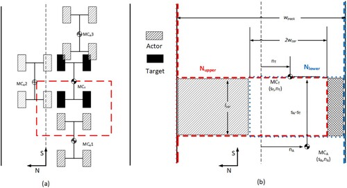
Different from the majority of collision-avoidance research that uses quadratic distance (i.e. a circle) to describe the collision exclusive zone [35], in this study the zone is rectangular with the front edge starting from the centre of the target car. The length of the rectangle is the same length as the car and the width is twice the car width laterally symmetrical about the target car centre. There are two main reasons to do so. First, it is to ensure a precise description of the collision zone so that no track space is overlooked which might lead to potential overtaking opportunities. Second, starting the front edge from the CG position of the target car aims to echo the second aforementioned main assumption that to overtake, the actor car only needs to pass the abreast position of the target car. The collision constraint is formulated as follows: (5) $\{\begin{array}{c}{N}_{upper}-n_A>0,\\ n_A-N_{lower}>0,\end{array}$(5) where the lateral boundaries $N_{upper}$ and $N_{lower}$ are given by (6) $\begin{array}{rl}{N}_{upper}& =\{\begin{array}{cc}0.5w_{road}& \text{if}{n}_T>n_A,\\ \begin{array}{c}0.5w_{road}+(w_{car}+0.5w_{road}-n_A)\\ (H(s_A-s_T)+H(s_A-s_T+l_{car}))\end{array}& \text{if }{n}_T\le n_A,\end{array}\end{array}$(6) (7) $\begin{array}{rl}{N}_{lower}& =\{\begin{array}{cc}\begin{array}{c}0.5w_{road}-(w_{car}+0.5w_{road}+n_A)\\ (H(s_A-s_T)+H(s_A-s_T+l_{car}))\end{array}& \text{if}{n}_T>n_A,\\ 0.5w_{road}& \text{if }{n}_T\le n_A,\end{array}\end{array}$(7) where $s$ and $n$ are the longitudinal and lateral position of a car on the track based on the curvilinear coordinate system. The subscripts $A$ and $T$ denote the actor car and the target car, respectively. $w_{car}$ and $l_{car}$ are the car width and length. $w_{road}$ is the road width. The function $H$ is the Heaviside step function.

Both upper bound $N_{upper}$ and lower bound $N_{lower}$ are based on the half road width. The relative lateral position $n_A$ and $n_T$ determines whether to add an offset (second) term to shift one side of the boundary to the opposite side of the rectangular zone and form a passage with the other boundary. As shown in Figure 3(b), if the actor car $M{C}_A$ is on the right-hand side of the target car $M{C}_T$, then the upper bound becomes the red dash line while the lower bound remains as the blue dash line. These two dash lines form the diamond filled area which is passable in this scenario. Vice versa, if the actor car $M{C}_A$ is on the left-hand side of the target car $M{C}_T$, then boundaries become the red and blue dot lines making the diagonal area passable. The collision constraint is active only when the actor car is within one car length behind the target car. If the actor car is further behind or has passed the abreast position, the constraint functions as normal road boundaries.

3. OCP formulation

The OCP is formulated in order to solve the problem of minimising the cost function in Bolza form, that is (8) $J=\mathrm{\varnothing }(t_0,x(t_0),t_f,x(t_f),p)+{\int }_{t_0}^{t_f}l(t,x(t),u(t),p)dt.$(8) Which is subject to the constraints of (9) $\{\begin{array}{c}{\displaystyle \frac{dx}{dt}}-f(t,x(t),u(t),p)=0,g(t,x(t),u(t),p)=0,\\ h(t,x(t),u(t),p)\le 0,\\ g_b(x(t_0),x(t_f),u(t_0),u(t_f),p)=0,\end{array}$(9) where the first term in Equation (29) is the Major (boundary) cost and the latter term is the Lagrange cost.

In this formulation, $p\in R^{n_p}$ denotes the constant parameter vector of $n_p$ dimensions to be optimised, $x(t)\in R^n$ is the state vector and $u(t)\in R^m$ is the control vector. The system dynamics is described in the vector $f(t,x(t),u(t),p)\in R^n$. Vector $g\in R^{n_g}$ and $g_b\in R^{n_{gb}}$ are the quality constraints and the constraints for the boundaries. The inequality constraints are defined in $h\in R^{n_h}$.

3.1. MTM and energy management

In Formula-E races, as previously introduced, energy management is one of the most crucial tasks in a race. Being faster or saving more energy is a dilemma and technically, there is no solution as ‘the fastest lap time with the lowest energy consumption’. In this study, the OCP is formulated in two ways for different analysis purposes. The first one is to find out the fastest lap time achievable with the presence of a target car in order to find possible overtaking opportunities along the full track length. The second one is to calculate the minimum energy required to perform a successful overtake.

For the MTM problem, the cost function will only contain the Lagrange stage cost which is (10) $J_{MTM}={\int }_{s_0}^{s_t}(Sf+ϵ{\dot{u}}^{T}W\dot{u})ds,$(10) where $Sf$ is the car travel time for $ds$ length along the track centreline, $s_0$ and $s_t$ are the initial and terminal length of the track, respectively. The term $ϵ{\dot{u}}^{T}W\dot{u}$ is a piece-wise derivative variation perturbation term that is added to the stage cost to regularise the problem. $W$ is a positive definite weight matrix, $\dot{u}$ and ${\dot{u}}^T$ denote the change rate of control vectors and their transposed form. $ϵ\in (10e-4,10e-2)$ is a very small value to minimise the effect of this term on time optimality. The function of this regularisation term is to avoid singular arcs and oscillation in the solution caused by the nature of numerical algorithms [36] and to improve convergence performance [37]. Similarly, for the energy management problem, the cost function is (11) $J_{EM}={\int }_{s_0}^{s_t}(P_{drive}-P_{regen}+ϵ{\dot{u}}^{T}W\dot{u})ds.$(11) In both problems, the system dynamics are included in $f(t,x(t),u(t),p)$, whereas the load transfer governing equations are treated as equality path constraints included in $g(t,x(t),u(t),p)$. And finally, the bounds for states and controls, and path constraints of power limit and collision constraint are included in the inequality constraints $h(t,x(t),u(t),p)$. The difference between the two problems is the time and energy. In the MTM problem, time is the objective to be minimised and energy is an integral boundary in inequality constraints $h(t,x(t),u(t),p)$ while in the energy management problem, time becomes an integral boundary: (12) $t_A={\int }_{s_0}^{s_t}Sfds<t_T-t_{gap},$(12)

which means that the actor finishing time $t_A$ needs to be shorter than the target car lap time $t_T$ by subtracting the initial time gap $t_{gap}$. In this way, the solver failing to generate a solution would suggest that overtaking under given constraints (e.g. low max energy consumption, big time gap) is infeasible. Note that the target car’s trajectory position $(s_T,n_T)$ is treated as a function of time in the problem formulation.

3.2. Scaling and mesh refinement

The OCP in this study is transcribed into a large non-linear programming problem (NLP) using Legendre–Gauss–Radau (LGR) quadrature orthogonal collocation method and Radau’s integration formula [38]. To implement this, the General-Purpose Optimal Control MATLAB Toolbox GPOPS-II [39] and underlying interior-point algorithm IPOPT [40] are used.

In addition to the regularisation term in Equations (31) and (32), scaling is another factor that can significantly affect the convergence performance of the optimisation algorithms. Instead of simply scaling into the range of [−0.5, 0.5], the base quantities can be scaled into dimensionless quantities in order to improve the NLP solver performance. In this study, the vehicle mass of 900 kg is scaled into a dimensionless value of 1. The car wheelbase of 3.1 m is taken as the fundamental unit of length and given the dimensionless value of 1. In order to define the scaler for time variables, the gravitational acceleration $g$ is scaled to the value of 1 so that the gravitational force of the car becomes the dimensionless value of 1. Using this method, other derived quantities such as the power of 250 kW now is 5.14, tyre normal force of 6000 N now is 0.68 and 50,000 J of energy is scaled to 1.8, etc. This method will scale the NLP’s variables in the original problem from a highly elongated hyperellipsoid into a more spherical space [36].

In GPOPS-II, a large OCP is segmented into mesh intervals and orthogonal collocation techniques are used in each mesh interval. Mesh refinement is a strong enhancement technique to improve the computational efficiency and accuracy of polynomial approximation in the mesh intervals. Varieties of hp methods have been developed in previous research [41–43] in which a mesh interval can be divided into multiple intervals (i.e. h method) and the degree of approximation polynomial in an interval can be increased (i.e. p method). In this study, the method proposed by Liu et al. [44] is used. While other methods might end up with an unnecessarily dense mesh or high-order polynomial, this method is able to (1) reduce the degree of polynomials when the high-order term in the power expansion is sufficiently small and (2) merge adjacent mesh intervals when the degree of approximation intervals inside these intervals is essentially the same. This feature will ease the computational burden created by either dense initial mesh setup or over-refined meshes during the optimisation iterations.

3.3. Smoothing function

The interior-point NLP algorithm assumes the constraint and object functions are continuously differentiable and it requires the first- and second-order derivative information. Therefore, the Heaviside step functions and if conditions in the collision constraints must be approximated in a smooth differentiable way. For this purpose, the Heaviside step function in the collision constraint is approximated using (13) $H(x)\approx H_s(x)=0.5+0.5\text{tanh}(kx).$(13) Similarly, the if condition can be described using the smoothed Heaviside step function $H_s(x)$. The collision boundaries of Equations (27) and (28) become (14) $\begin{array}{rl}{N}_{upper}& =0.5w_{road}+(w_{car}+0.5w_{road}-n_A)\\ & \times (H_s(s_A-s_T)+H_s(s_A-s_T+l_{car}))H_s(n_A-n_T),\end{array}$(14) (15) $\begin{array}{rl}{N}_{lower}& =0.5w_{road}-(w_{car}+0.5w_{road}+n_A)\\ & \times (H_s(s_A-s_T)+H_s(s_A-s_T+l_{car}))H_s(n_T-n_A).\end{array}$(15)

The accuracy of such approximation improves when the $k$ value increases. To ensure that the approximation does not change the original problem significantly, $k\in (1e2,1e4)$ is used in this paper.

4. Results and discussion

The problems are solved on a local machine with i7-6700HQ processor. Using the MATLAB-based transcription code and C++ NLP solver, the average solution time of a single case in this study is around 50 min. It has been shown in [45] that the solution time can be significantly reduced (13–50%) by implementing the algorithms entirely in C++ due to higher code efficiency. This is not the main focus of this study, thus is not discussed further.

The results shown in this section are collected from cases of different performances (due to different EPL constraints) of the target car and various gaps. These results are presented in two aspects. The first one shows the successful overtaking manoeuvres at different locations on the track found in the solutions. The second one demonstrates the feasibility of overtaking manoeuvres and the energy penalty that needs to be paid if feasible.

4.1. Overtaking manoeuvres

To demonstrate potential overtaking opportunities, we use a reference trajectory from a car with a 1.4 kWh energy constraint and 200 kW power constraint as an example. The problem is formulated using the cost function of Equation (31) which is a simple MTM problem. The actor car is given the same 200 kW power constraint but with no energy constraint. We swept through a range of head start gaps that we gave to the target car, from 0.1 s until no overtaking can be observed. From the result collected, on the Marrakesh track, the majority of the successful overtaking manoeuvres take place in the highlighted sectors shown in Figure 4(a).

Figure 4. (a) Observed overtaking positions(highlighted in ) and (b) example speed profile using LaC.

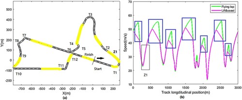
Figure 4(b) demonstrates two examples of speed profiles. The purple line is from a car doing LaC with a 1.4 kWh energy per lap constraint whereas the green one does not have any energy constraint applied. By comparing Figure 4(a) and (b), it can be observed that most of the overtaking manoeuvres happened in the areas where the target car used the LaC technique to save its energy (bold blue blocks). One exceptional case was found in the Z1 area marked in Figure 4(a) and (b) where the actor car successfully overtook when both cars were fully accelerating. This manoeuvre is shown in detail in Figure 5.

Figure 5. Overtaking at turn one: (a) car trajectories and (b) speed profile and relative position.

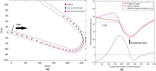
Figure 5 shows an overtaking between the first and second corners (Z1 area in Figure 4). This is a case where both cars are under race mode setting (200 kW power) with a small initial time gap (0.1 s). At the start, the target car was leading by a 0.1-second gap. As is shown in Figure 5(b), while the target car started to lift and coast (LaC), the actor car continued to accelerate and got in front of the target car. The high speed of the actor car during entering the corner forced it to go wide in the corner and give back the leading position to the target car. However, this temporary loss in return gave the actor car an opportunity to accelerate earlier than the target and established a speed advantage when exiting the corner. Given the speed advantage, the actor car then successfully overtook the target soon after exiting turn one.

Another unique overtaking manoeuvre (in a different simulation) was found featuring the activation of attack mode. This is shown in Figure 6.

Figure 6. Overtaking at turn three: (a) car trajectories and (b) speed profile and relative position.

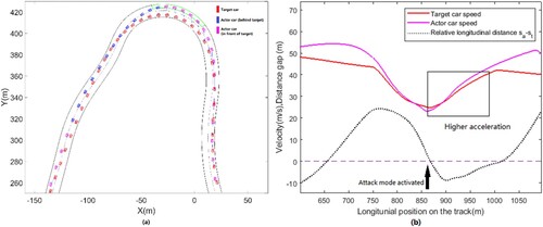
In this case, the target car was on a normal race mode lap with 1.4 kWh energy consumption while the actor car is in an attack mode activation lap in which it has to drive through the activation zone (shown by green colour in Figure 6(a)) to be entitled to the extra 50 kW power output. The actor car was leading before entering the activation zone and lost its position due to the target car taking a tighter line. After the attack mode was activated, the higher power of the actor car allowed it to accelerate faster than the target car as is shown in Figure 6(b). The actor car regained its leading position soon after exiting turn three and is then able to further build up the leading gap.

The rest of the overtaking manoeuvres found are generally simple ones where the actor car takes advantage of the speed difference over the target car doing LaC before entries of corners. They are of less interesting features which are shown in Appendix C instead of this section.

4.2. Energy consumption of overtaking laps

In this section, the problem is formulated in the way of Equation (32) with lap time being a boundary as stated in Equation (33). In this way, the objective is to find the minimum energy required to execute a successful overtaking (imposed by Equation (33)) given different initial time gaps between the target and actor car. Failure of solving a scenario means the overtaking is fundamentally infeasible in that given scenario (e.g. initial gap, high target car energy allowance).

As previously introduced, a car has three possible power modes featuring different power limits. An overtaking attempt is considered rational only when the actor car has higher or at least equal power compared to the target car. This gives six different basic scenarios as presented in Table 1.

Table 1. Overtaking scenarios.

Scenario	Actor car power mode (power limit)	Target car power mode (power limit)
S1	Race mode (200 kW)	Race mode (200 kW)
S2	Activation lap (200/250 kW)^a	Race mode (200 kW)
S3	Attack mode (250 kW)	Race mode (200 kW)
S4	Attack mode (250 kW)	Activation lap (200/250 kW)^a
S5	Activation lap (200/250 kW)^a	Activation lap (200/250 kW)^a
S6	Attack mode (250 kW)	Attack mode (250 kW)

^a In an activation lap, the power limit is 200 kW before the activation zone and 250 kW afterwards.

In each scenario, we use a series of target car trajectories obtained under different energy constraints (1.2–2 kWh). With each reference trajectory, we complete a number of simulations over a sweep of initial gaps starting from 0.1 s with 0.1 s increment until the solver fails to generate a solution or a maximum gap of 3 s is reached.

In this section, only S1, S2, S3, S4 are shown due to some unique features found in the solutions. Results of S5 and S6 are shown in Appendix D. Figure 7 shows the minimum energy requirement in different scenarios with different initial time gaps and target car energy usage.

Figure 7. Minimum energy consumption for a successful overtaking lap: (a) scenario S1; (b) scenario S2; (c) scenario S3; (d) scenario S4. The red lines categorise the simulations into two groups. On the left-hand side, the actor car can overtake the target using less energy than the target car. The right-hand side is the opposite.

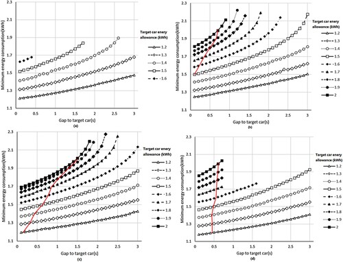
In terms of energy consumption, it is natural that the energy requirement increases when the target has a bigger advantage of either a bigger initial gap or a higher energy allowance. This correlation becomes non-linear and increases sharply with a bigger target advantage. However, an energy-efficient way of overtaking can be found when the actor car is on a higher power limit setting than the target car. As marked by red lines in Figure 7(b–d), the region on the left-hand side of the red lines lies the cases in which the actor car can overtake the target using less energy than the target. This is due to the fact that higher power contributes to the performance in a significantly efficient way as pointed out in [27]. The power limit in [27] and this study is modelled as a path constraint in the OCP which means that the car is allowed to explore any power below the limit. When given an energy constraint, the fact that the solutions suggest doing lift and coasting instead of lowering the power indicates that the objective is more sensitive to the power limit. This can also be interpreted in the other way that a higher power limit is beneficial given the same or even tighter energy constraint. In contrast as shown in figure of scenario S1, when two cars have the same power settings, the actor has no other way but to use more energy to create speed advantages in order to overtake the target considering that the target is already on its optimal usage of energy.

It can be observed in Figure 7 that successful overtaking solutions were found across the full-time gap range when the target car energy allowance is low (e.g. 1.2, 1.3 kWh/lap). However, when the target car was given more energy, solutions could not be found in the higher range of time gaps or even with the smallest gap of 0.1 s. There are two main causes for such results. First, the target car with a higher energy allowance naturally does less LaC. This is the reason why no solutions can be found when the target car has more than 1.7 kWh/lap of energy as shown in Figure 7(a) under scenario S1. In such cases, although the target car still does LaC which potentially gives the actor a speed advantage (demonstrated in Figure 4), the window of LaC is too short that the actor cannot gain enough speed advantage to overtake without violating the collision constraint (Figure 3). Second, although knowing overtaking is possible with the target car given a certain amount of energy, the initial gap might be too big that the actor car is unable to catch up with the target before reaching the last possible overtaking zone. This can be further demonstrated in Figure 8 which shows the longitudinal distance between the actor and target car of the cases.

Figure 8. The relative position of the actor and target cars: (a) scenario S4 with target car energy allowance of 1.4kWh and (b) scenario S4 with target car energy allowance of 1.7kWh. Turn numbers are marked corresponding to Figure 4(a).

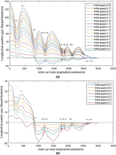
In Figure 8, the relative position crossing zero denotes that overtaking occurs. It is noticeable from the figure that the overtaking position varies with different initial time gaps. Considering the problem formulation which aims to find the minimum energy consumption in overtaking, that feature means that the most energy-efficient overtaking position changes with a different initial gap. For the cases shown in Figure 8(a), when the initial gap is less than 0.7 s, the overtaking manoeuvres take place at turn three. As the initial gap increases, the overtaking position is postponed to the highlighted zone before turn 11. When the gap is larger than 1.5 s, the overtaking is suggested to be executed in the highlighted zone before turn 12. Such results demonstrated in Figure 8 can be interpreted in two ways. First, in the cases with larger initial gaps, the solutions suggest that to accomplish overtaking within a lap using the least possible amount of energy, the actor car does not have to overtake as early as possible. This indicates that rushing to earlier overtaking positions is not an energy-efficient solution. However, this does not mean the overtaking should be postponed until the last possible position which leads to the second interpretation that for scenario S4, the most energy-wise ideal overtaking position is at turn 3. With the smallest initial gap of 0.1 s, which is the bottom blue line in Figure 8(a), the actor theoretically has many overtaking chances along the full track. The solution suggests overtaking at turn three instead of following the target car for later overtaking chances which indicates the superiority of turn three. This can also be explained together with Figure 6(a). In scenario S4, the target car needs to drive into the activation zone at turn three, clearing the normal racing line for the actor car. If the actor car can catch up efficiently before turn three then it can use such position advantage to overtake while driving on its optimal line with less concern about the collision constraints. Otherwise, the actor car needs to deliberately create a speed advantage later using more energy in order to overtake the actor which occupies the optimal race line. Therefore, turn three proves to be a very favourable overtaking position.

Figure 8(b) shows the cases where the target car is given more energy hence less LaC operations. As a result, this leaves the actor car no chance of overtaking after turn three because the actor will not be able to create enough speed advantage. Therefore, turn three becomes the last overtaking opportunity. If the actor cannot catch up with the target due to large initial gaps, then there is no overtaking chance in such a lap. This also explains the sharp cut in Figure 7(d), that overtaking is infeasible when the target car is given more than 1.6 kWh of energy and the initial gap is larger than 0.7 s.

Additionally, as it can be observed in Figure 7 and Appendix C for scenarios S1, S5 and S6, when the target car is given a very high energy allowance meantime under the same power limit as the actor car, overtaking is very difficult and mostly infeasible. Such cases can be referred to as safe scenarios where one cannot be overtaken despite an opponent being willing to spend more energy. However, it should be noted that such results are based on the assumptions introduced in Section 2.3.3. In real life, overtaking might still be possible in these safe scenarios if a driver decides to overtake aggressively by blocking or forcing the opponent car off its race line. These manoeuvres might lead to danger or penalties thus are not discussed in this study. Additional overtake trajectories are shown in Appendix B.

5. Conclusion

In this study, the overtaking feasibility and energy consumption of formula E cars were analysed by formulating an OCP. Multiple overtaking opportunities were found along the full length of a track. An overtaking can be feasible under three circumstances. (1) Actor car gaining speed advantage by doing less LaC than target car. (2) Actor car gaining speed advantage with a higher power limit than target car. (3) Target car deviating from the normal race line leaving track space for actor car. However, when the target car is on a high energy consumption lap (i.e. faster with less LaC), overtaking might start to be infeasible. The infeasibility might also happen when the initial gap is too large for the actor car to catch up with the target before reaching the last possible overtaking position. In such scenarios, the target car can be considered as in a safe position.

In terms of minimum energy consumption of an overtaking lap, the most energy-efficient position varies with different initial time gaps and energy consumption of the target car. When the actor and target cars are under the same power limit, the actor needs to use additional energy to execute overtaking and the amount increases as the initial gap gets larger. If the actor car is on a higher power mode setting than the target, an overtaking lap can be performed using less energy than the target making it a very efficient strategy.

Overall, it is proved that choice of when and where to overtake an opponent significantly influences overtaking feasibility and energy consumption. Such decisions are a crucial element in Formula-E race strategy on a multi-lap level. This paper offers insight analysis of overtaking and fills the gap of multi-car lap performance analysis in the literature.

Disclosure statement

No potential conflict of interest was reported by the authors.

Appendix

Appendix A. Track and vehicle modelling

A.1. Track modelling

In this paper, the curvilinear coordinate system is used to describe the track. The travelled distance $s$ from the start/finish line to a certain point is treated as abscissa and corresponded to the curvature $C$ of that point. As shown in Figure A1.

Figure A1. Track curvilinear coordinates.

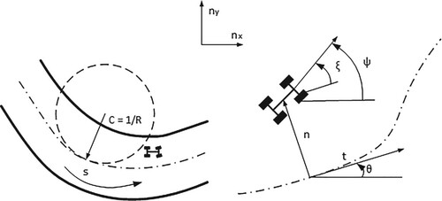
Therefore, the position of the car is described using $s$ and $n$ which is the perpendicular distance of the vehicle mass centre from the centreline to the centreline’s tangent direction. They are calculated using their derivatives: (A1) $\begin{array}{rl}\dot{s}& =\frac{u\text{ cos}\xi -v\text{ sin}\xi }{1-nC},\end{array}$(A1) (A2) $\begin{array}{rl}\dot{n}& =u\text{ sin}\xi +v\text{ cos}\xi ,\end{array}$(A2) where $u$ and $v$ are the longitudinal and lateral velocity of the vehicle, respectively. ξ describes the relation between the vehicle heading direction and the track centreline tangent direction and is calculated by (A3) $\dot{\xi }=\dot{\psi }-C\dot{s}$(A3) in which $\dot{\psi }=\omega$ is the vehicle yaw rate and will be later used in vehicle modelling. It should be noted that the dot notation denotes that these are time derivatives. In this paper, travelled distance $s$ is assumed to be a monotonically increasing function of time due to the fact that in motorsport, cars are not supposed to reverse or head backwards on the track. And because overtaking is a manoeuvre directly related to positions, in the OCP, $s$ is used as the independent variable instead of time. To convert the time derivatives into ones with respect to distance (A4) $ds=\frac{ds}{dt}dt=\frac{u\text{ cos}\xi -v\text{ sin}\xi }{1-nC}dt$(A4) we define $S_f$ representing the reciprocal of velocity of vehicle along the track centreline as (A5) $S_f={\left(\frac{ds}{dt}\right)}^{-1}=\frac{1-nC}{u\text{ cos}\xi -v\text{ sin}\xi }.$(A5) Therefore, the lateral position of the vehicle $n$ and angle ξ can be calculated by (A6) $\begin{array}{rl}\frac{dn}{ds}& =(u\text{ sin}\xi +v\text{ cos}\xi )S_f,\end{array}$(A6) (A7) $\begin{array}{rl}\frac{d\xi }{ds}& =S_f\omega -C.\end{array}$(A7) It should be noted that in this paper, positive values of $\omega$ and $C$ denote an angular change in anti-clockwise. Positive $n$ and $v$ denote travel to the left-hand side.

A.2. Vehicle modelling

Traditionally, the high-fidelity vehicle models are usually used as a validation tool to test a strategy that is established through optimisations beforehand. A classic development procedure can be demonstrated by the schematic shown in Figure A2. This study focuses on steps 1 and 2, which lay the foundation for high-fidelity validations. For the benefit of computational cost while maintaining the essential characteristics of the car mentioned in Section 2, the vehicle model is described by seven DOFs.

Figure A2. Classic developing procedure.

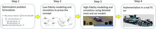
Figure A3. 7 DOF Vehicle model

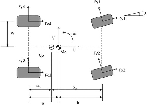
A.2.1. Body dynamics

As illustrated in Figure A3, the longitudinal, lateral and yaw motions of the body can be calculated using the following equations: (A8) $\begin{array}{rl}M\frac{d}{dt}u(t)& =M\omega v+F_x,\end{array}$(A8) (A9) $\begin{array}{rl}M\frac{d}{dt}v(t)& =-M\omega u+F_y,\end{array}$(A9) (A10) $\begin{array}{rl}{I}_z\frac{d}{dt}\omega (t)& =a(\text{cos}\delta (F_{y1}+F_{y2})+\text{sin}\delta (F_{x1}+F_{x2}))-w(\text{sin}\delta F_{y2}-\text{cos}\delta F_{x2})\\ & +w{F}_{x3}-w(\text{cos}\delta F_{x1}-\text{sin}\delta F_{y1})-w{F}_{x1}-b(F_{y3}+F_{y4}).\end{array}$(A10)

The descriptions of the symbols and numerical values are presented in Table A1.

Table A1. Symbols and descriptions.

Symbol	Description	Value
$M$	Vehicle mass	900 kg
$I_z$	Moment of inertia about the z-axis	450 kg m^2
$\delta$	Front wheel steering angle	Input
$w$	Half track width	0.775 m
$a$	Distance from the vehicle mass centre to the front axle	1.86
$b$	Distance from the vehicle mass centre to the rear axle	1.24 m

The $F_{xi}$ and $F_{yi}$ are the longitudinal and lateral forces, respectively, generated by the tyres with subscript i (i = 1,2,3,4) denoting the tyre on the front left, front right, rear right and rear left corner. The total longitudinal and lateral forces $F_x$ and $F_y$ acting on the vehicle, are given by $F_x=\text{cos}\delta (F_{x1}+F_{x2})-\text{sin}\delta (F_{y1}+F_{y2})+(F_{x3}+F_{x4})-F_{ax},$ $F_y=\text{ cos}\delta (F_{y1}+F_{y2})+\text{sin}\delta (F_{x1}+F_{x2})+(F_{y3}+F_{y4}),$where $F_{ax}$ is the longitudinal aerodynamic load on the car which will be defined in the following section.

A.2.2. Wheel dynamics and tyre normal loads

Each wheel has its DOF of rotation. These motions can be described using the following equations: (A11) $\begin{array}{rl}{J}_w\dot{{\omega }_1}& =k_b{T}_{brake}-F_{x1}R,\end{array}$(A11) (A12) $\begin{array}{rl}{J}_w\dot{{\omega }_2}& =k_b{T}_{brake}-F_{x2}R,\end{array}$(A12) (A13) $\begin{array}{rl}{J}_w\dot{{\omega }_3}& =T_{drive}+(1-k_b)T_{brake}-T_{diff\mathrm{\_}r}-F_{x3}R,\end{array}$(A13) (A14) $\begin{array}{rl}{J}_w\dot{{\omega }_4}& =T_{drive}+(1-k_b)T_{brake}+T_{diff\mathrm{\_}r}-F_{x4}R.\end{array}$(A14)

In which $J_w$ is the wheel rotational inertia, $k_b$ is the brake bias to the front, $T_{drive}$ and $T_{brake}$ are drive torque from the motor brake torque generated by the caliper or the motor regeneration, $R$ is the tyre radius.

The $T_{diff\mathrm{\_}r}$ is the LSD torque transferred from the faster-rotating wheel to the slower wheel. This torque is given by (A15) $T_{diff}=0.5k_d({\omega }_{inner}-{\omega }_{outer}),$(A15) where ${\omega }_{inner}$ and ${\omega }_{outer}$ are the wheel angular velocities of the inner and outer wheel on the same axle and $k_d$ is the rotational damping coefficient of the LSD.

The tyre model used in this paper is an empirical tyre model [46] and uses linearised interpolation [47] to describe the change of peak values of longitudinal and lateral friction coefficient due to normal load variations. The detailed model is shown in Appendix A. The normal forces acting on the tyres must satisfy the balancing equations as follows.

In the vertical direction, (A16) $F_{z1}+F_{z2}+F_{z3}+F_{z4}-Mg-F_{az}=0,$(A16) where $F_{zi}$ are the tyre normal force on each tyre. $g$ is the acceleration due to gravity and $F_{az}$ is the aerodynamic vertical load on the car.

To balance the moment around the x-axis and y-axis (illustrated in Figure A3) of a car, (A17) $\begin{array}{rl}& w(F_{z4}-F_{z3})+w(F_{z1}-F_{z2})+F_y=0,\end{array}$(A17) (A18) $\begin{array}{rl}& b(F_{z3}+F_{z4})-a(F_{z1}+F_{z2})-h{F}_x-(a_A-a)F_{az}=0.\end{array}$(A18) In which h is the height of the vehicle mass centre to the ground.

To ensure a unique solution for the four normal forces, a fourth balancing equation is formulated by introducing the lateral load transfer bias $D$ which describes the lateral load transfer distribution between the front and rear axle (A19) $D(F_{z2}+F_{z3}-F_{z1}-F_{z4})-F_{z2}+F_{z1}=0.$(A19) The aero loads $F_{az}$ and $F_{ax}$ are given by (A20) $\begin{array}{rl}{F}_{az}& =0.5C_l{\rho }_{a}A{u}^2,\end{array}$(A20) (A21) $\begin{array}{rl}{F}_{ax}& =0.5C_d{\rho }_{a}A{u}^2.\end{array}$(A21) In which $C_d$ and $C_l$ are the aerodynamic coefficient of drag and lift, ${\rho }_a$ is the air density and $A$ is the frontal area of the car.

Appendix B. Tyre model

The tyre model used in this paper is an empirical tyre model with linearised interpolation for peak values of longitudinal and lateral friction coefficients. The longitudinal and lateral forces are given by (B1) $\begin{array}{rl}{F}_{xi}& ={\mu }_{xi}{F}_{zi}\frac{{\kappa }_{ni}}{\sqrt{{\alpha }_{ni}^2+{\kappa }_{ni}^2+ϵ}},\end{array}$(B1) (B2) $\begin{array}{rl}{F}_{yi}& ={\mu }_{yi}{F}_{zi}\frac{{\alpha }_{ni}}{\sqrt{{\alpha }_{ni}^2+{\kappa }_{ni}^2+ϵ}},\end{array}$(B2) where $F_{zi}$ is the tyre normal force, ${\kappa }_{ni}$ and ${\alpha }_{ni}$ are the normalised tyre slip with respect to the slip value where peak friction coefficient happens: (B3) $\begin{array}{rl}{\alpha }_{ni}& =\frac{{\alpha }_i}{{\alpha }_{maxi}},\end{array}$(B3) (B4) $\begin{array}{rl}{\kappa }_{ni}& =\frac{{\kappa }_i}{{\kappa }_{maxi}}.\end{array}$(B4) The slip angles ${\alpha }_{ni}$ and ratios ${\kappa }_{ni}$ are given by (B5) $\begin{array}{rl}{\alpha }_1& =\delta -\text{arctan}\left(\frac{v+\omega a}{u-\omega w}\right),{\kappa }_1=-1+\frac{R{\omega }_1}{\text{cos}\delta (u-\omega w)-\text{sin}\delta (v+\omega a)},\end{array}$(B5) (B6) $\begin{array}{rl}{\alpha }_2& =\delta -\text{arctan}\left(\frac{v+\omega a}{u+\omega w}\right),{\kappa }_2=-1+\frac{R{\omega }_2}{\text{cos}\delta (u+\omega w)-\text{sin}\delta (v+\omega a)},\end{array}$(B6) (B7) $\begin{array}{rl}{\alpha }_3& =-\text{arctan}\left(\frac{v-\omega b}{u+\omega w}\right),{\kappa }_3=-1+\frac{R{\omega }_3}{u+\omega w},\end{array}$(B7) (B8) $\begin{array}{rl}{\alpha }_4& =-\text{arctan}\left(\frac{v-\omega b}{u-\omega w}\right),{\kappa }_4=-1+\frac{R{\omega }_4}{u-\omega w}.\end{array}$(B8)

In which ${\omega }_i$ is the angular velocity of each wheel and R the tyre radius.

The peak friction values are given by linear interpolation which treats them as a linear function or the tyre normal loads. The symbols are explained in Table B1. (B9) $\begin{array}{rl}{\mu }_{xmax}& =(F_z-F_{zR1})\left(\frac{{\mu }_{xmax2}-{\mu }_{xmax1}}{F_{zR2}-F_{zR1}}\right)+{\mu }_{xmax1},\end{array}$(B9) (B10) $\begin{array}{rl}{\mu }_{ymax}& =(F_z-F_{zR1})\left(\frac{{\mu }_{ymax2}-{\mu }_{ymax1}}{F_{zR2}-F_{zR1}}\right)+{\mu }_{ymax1},\end{array}$(B10) (B11) $\begin{array}{rl}{\kappa }_{max}& =(F_z-F_{zR1})\left(\frac{{\kappa }_{max2}-{\kappa }_{max1}}{F_{zR2}-F_{zR1}}\right)+{\kappa }_{max1},\end{array}$(B11) (B12) $\begin{array}{rl}{\alpha }_{max}& =(F_z-F_{zR1})\left(\frac{{\alpha }_{max2}-{\alpha }_{max1}}{F_{zR2}-F_{zR1}}\right)+{\alpha }_{max1}.\end{array}$(B12)

Table B1. Description of symbols.

Symbol	Description	Front value	Rear value
$F_{zR1}$	Reference normal load 1	2000 N	2000 N
$F_{zR2}$	Reference normal load 2	6000 N	6000 N
${\mu }_{xmax1}$	Peak longitudinal friction coefficient at load 1	1.4	1.75
${\mu }_{xmax2}$	Peak longitudinal friction coefficient at load 2	1.12	1.4
${\kappa }_{max1}$	Slip coefficient for the friction peak at load 1	0.11	0.11
${\kappa }_{max2}$	Slip coefficient for the friction peak at load 2	0.10	0.10
${\mu }_{ymax1}$	Peak lateral friction coefficient at load 1	1.62	1.8
${\mu }_{ymax2}$	Peak lateral friction coefficient at load 2	1.3	1.45
${\alpha }_{max1}$	Slip angle for the friction peak at load 1	9°	9°
${\alpha }_{max2}$	Slip angle for the friction peak at load 2	8°	8°
$Q_x$	Longitudinal shape factor	1.9	1.9
$Q_y$	Lateral shape factor	1.9	1.9

Next, the longitudinal and lateral friction coefficients in Equations (B1) and (B2) are described by (B13) $\begin{array}{rl}{\mu }_{xi}& ={\mu }_{ximax}\sin \left(Q_x\arctan \left(\frac{\pi }{2\arctan (Q_x)}\sqrt{{\alpha }_{ni}^2+{\kappa }_{ni}^2}\right)\right),\end{array}$(B13) (B14) $\begin{array}{rl}{\mu }_{yi}& ={\mu }_{yimax}\sin \left(Q_y\arctan \left(\frac{\pi }{2\arctan (Q_y)}\sqrt{{\alpha }_{ni}^2+{\kappa }_{ni}^2}\right)\right),\end{array}$(B14) where $Q_x$ and $Q_y$ are shaping factors.

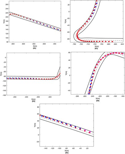
Appendix C. Additional overtaking trajectories

Figure C1. Overtaking trajectories at different positions of the track. B1: before turn seven, B2: before turn 10, B3: before turn 11, B4: before turn 12, B5: before finishing line, red block: target car, blue block: actor car before overtaking, purple block: actor car after overtaking.

Appendix D. Complementary results of minimum energy consumption analysis

To demonstrate that the proposed approach is robust to change of vehicle parameters, we reduced the ${\mu }_{xmax1}$, ${\mu }_{xmax2}$, ${\mu }_{ymax1}$ and ${\mu }_{ymax2}$ in the tyre model by 10% to simulate a slippery track condition which in real life is likely to be caused by rain or dust. Scenarios S1 and S6 are shown in Figure D2.

It can be observed that the general trends of energy consumption are similar with increasing consumption and a limit where overtaking is no longer feasible. By comparing Figure D1(right) and D2(right) under the same scenario, it can be seen that the slippery condition increases the energy cost of overtaking and also the target car is safer with lower EPL (overtaking is not feasible with EPL higher than 1.5 kWh). It should be noted that in the slippery scenarios, the reference car trajectories were also regenerated based on the reduced-coefficient tyre model.

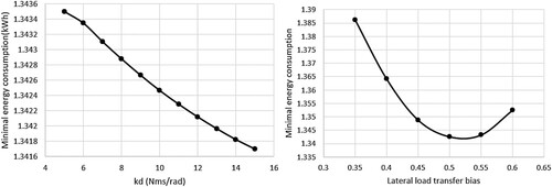
This figure shows an example of the resulting sensitivity of a particular case in scenario S6 with a slippery track condition where the target car uses 1.2 kWh of energy and the initial gap is 1.5 s. Two of the common vehicle setting parameters in the seven DOFs vehicle model are shown, namely the rotational damping coefficient of LSD in Equation (A15) and the lateral load transfer bias in Equation (A19). It should be noted that one of the strengths of formulating such an OCP is that such vehicle parameters can be optimised simultaneously by including them in $p\in R^{n_p}$ in Equation (30). With such a method, for each case, only a single simulation is needed instead of sweep simulations.

Figure D1. Minimum energy consumption for a successful overtaking lap (left) scenario S5 and (right) scenario S6.

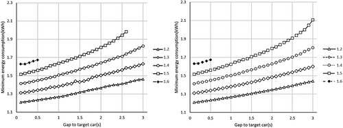
Figure D2. Minimum energy consumption for a successful overtaking lap on a slippery track condition (left) scenario S1 and (right) scenario S6.

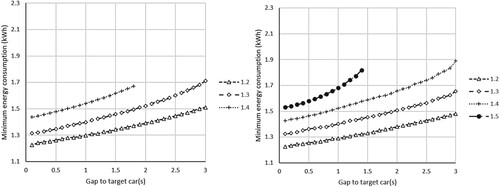
Figure D3. Minimum energy consumption sensitivity example (left) rotational damping coefficient of LSD (right) the lateral load transfer bias.

References

- Butz MV, Lonneker TD. Optimized sensory-motor couplings plus strategy extensions for the torcs car racing challenge. 2009 IEEE Symposium on Computational Intelligence and Games. IEEE; 2009.
- Cardamone L, Loiacono D, Lanzi PL. On-line neuroevolution applied to the open racing car simulator. 2009 IEEE Congress on Evolutionary Computation. IEEE; 2009.
- Quadflieg J, Preuss M, Rudolph G. Driving faster than a human player. European Conference on the Applications of Evolutionary Computation. Berlin, Heidelberg: Springer; 2011.
- Butz MV, Linhardt MJ, Lonneker TD. Effective racing on partially observable tracks: indirectly coupling anticipatory egocentric sensors with motor commands. IEEE Trans Comput Intell AI Games. 2010;3(1):31–42.
- Onieva E, Cardamone L, Loiacono D, et al. Overtaking opponents with blocking strategies using fuzzy logic. Proceedings of the 2010 IEEE Conference on Computational Intelligence and Games. IEEE; 2010.
- Loiacono D, Prete A, Lanzi PL, et al. Learning to overtake in TORCS using simple reinforcement learning. IEEE Congress on Evolutionary Computation. IEEE; 2010.
- Huang H-H, Wang T. Learning overtaking and blocking skills in simulated car racing. 2015 IEEE Conference on Computational Intelligence and Games (CIG). IEEE; 2015.
- Kitazawa S, Kaneko T. Control target algorithm for direction control of autonomous vehicles in consideration of mutual accordance in mixed traffic conditions. Proceedings of the 13th International Symposium on Advanced Vehicle Control. 2016.
- Glaser S, Vanholme B, Mammar S, et al. Maneuver-based trajectory planning for highly autonomous vehicles on real road with traffic and driver interaction. IEEE Trans Intell Transp Syst. 2010;11(3):589–606.
- Shim T, Adireddy G, Yuan H. Autonomous vehicle collision avoidance system using path planning and model-predictive-control-based active front steering and wheel torque control. Proc Inst Mech Eng. Part D: J Autom Eng. 2012;226(6):767–778.
- Ma L, Xue J, Kawabata K, et al. A fast RRT algorithm for motion planning of autonomous road vehicles. 17th International IEEE Conference on Intelligent Transportation Systems (ITSC). IEEE; 2014.
- Katrakazas C, Quddus M, Chen W-H, et al. Real-time motion planning methods for autonomous on-road driving: state-of-the-art and future research directions. Transp Res C Emerg Technol. 2015;60:416–442.
- Yuan J, Chen H, Sun F, et al. Trajectory planning and tracking control for autonomous bicycle robot. Nonlinear Dyn. 2014;78(1):421–431.
- Yue M, Hou X, Gao R, et al. Trajectory tracking control for tractor-trailer vehicles: a coordinated control approach. Nonlinear Dyn. 2018;91(2):1061–1074.
- Chu K, Lee M, Sunwoo M. Local path planning for off-road autonomous driving with avoidance of static obstacles. IEEE Trans Intell Transp Syst. 2012;13(4):1599–1616.
- Zhang L, Gao H, Chen Z, et al. Multi-objective global optimal parafoil homing trajectory optimization via Gauss pseudospectral method. Nonlinear Dyn. 2013;72(1-2):1–8.
- Gao Y, Gray A, Frasch JV, et al. Spatial predictive control for agile semi-autonomous ground vehicles. Proceedings of the 11th International Symposium on Advanced Vehicle Control, No. 2. 2012.
- Regulations. Federation Internationale De L'Automobile. Available from: http://www.fia.com/regulation/category/110.2022.6.22.
- Regulations. Federation Internationale De L'Automobile. Available from: http://www.fia.com/regulation/category/109.2022.
- Perantoni G, Limebeer DJ. Optimal control for a formula one car with variable parameters. Veh Syst Dyn. 2014;52(5):653–678.
- Perantoni G, Limebeer DJ. Optimal control of a formula one car on a three-dimensional track—part 1: track modeling and identification. J Dyn Syst Meas Contr. 2015;137(5):051018–051029.
- Tremlett AJ, Massaro M, Purdy DJ, et al. Optimal control of motorsport differentials. Veh Syst Dyn. 2015;53(12):1772–1794.
- Tremlett AJ, Limebeer DJN. Optimal tyre usage for a formula one car. Veh Syst Dyn. 2016;54(10):1448–1473.
- Limebeer DJ, Perantoni G, Rao AV. Optimal control of formula one car energy recovery systems. Int J Control. 2014;87(10):2065–2080.
- Ebbesen S, Salazar M, Elbert P, et al. Time-optimal control strategies for a hybrid electric race car. IEEE Trans Control Syst Technol. 2017;26(1):233–247.
- Herrmann T, Christ F, Betz J, et al. Energy management strategy for an autonomous electric racecar using optimal control. 2019 IEEE Intelligent Transportation Systems Conference (ITSC). IEEE; 2019.
- Liu X, Fotouhi A, Auger DJ. Optimal energy management for formula-E cars with regulatory limits and thermal constraints. Appl Energy. 2020;279:115805–115824.
- Liu X, Fotouhi A. Formula-E race strategy development using artificial neural networks and Monte Carlo tree search. Neural Comput Appl. 2020;32(18):1–17.
- Masouleh MI, Limebeer DJ. Optimizing the aero-suspension interactions in a formula one car. IEEE Trans Control Syst Technol. 2015;24(3):912–927.
- Dal Bianco N, Bertolazzi E, Biral F, et al. Comparison of direct and indirect methods for minimum lap time optimal control problems. Veh Syst Dyn. 2019;57(5):665–696.
- Gitlin JM. Formula E's new electric car looks like nothing else in racing. Ars Technica [Internet] 2018 Jan 30, 4:36 pm UTC. Available from: arstechnica.com/cars/2018/01/formula-es-new-electric-car-looks-like-nothing-else-in-racing/.2022.6.22.
- Mitchell S. Why formula E is so hard – autosport engineering. Autosport.com [Internet]. Available from: www.autosport.com/engineering/feature/8211/why-formula-e-is-so-hard0.2022.6.22.
- Viana ÍB, Kanchwala H, Aouf N. Cooperative trajectory planning for autonomous driving using nonlinear model predictive control. 2019 IEEE International Conference on Connected Vehicles and Expo (ICCVE). IEEE; 2019.
- You F, Zhang R, Lie G, et al. Trajectory planning and tracking control for autonomous lane change maneuver based on the cooperative vehicle infrastructure system. Expert Syst Appl. 2015;42(14):5932–5946.
- Hayashi R, Isogai J, Raksincharoensak P, et al. Autonomous collision avoidance system by combined control of steering and braking using geometrically optimised vehicular trajectory. Veh Syst Dyn. 2012;50(Supp1):151–168.
- Masouleh MI. Optimal control and stability of four-wheeled vehicles [dissertation]. Oxford: University of Oxford; 2017.
- Schwartz AL. Theory and implementation of numerical methods based on Runge–Kutta integration for solving optimal control problems [dissertation]. Berkeley: University of California; 1996.
- Davis PJ, Rabinowitz P. Methods of numerical integration. New York: Courier Corporation; 2007.
- Patterson MA, Rao AV. GPOPS-II: a MATLAB software for solving multiple-phase optimal control problems using hp-adaptive Gaussian quadrature collocation methods and sparse nonlinear programming. ACM Trans Math Softw (TOMS). 2014;41(1):1–37.
- Wächter A, Biegler LT. On the implementation of an interior-point filter line-search algorithm for large-scale nonlinear programming. Math Program. 2006;106(1):25–57.
- Patterson MA, Hager WW, Rao AV. A ph mesh refinement method for optimal control. Optim Control Appl Methods. 2015;36(4):398–421.
- Darby CL, Hager WW, Rao AV. Direct trajectory optimization using a variable low-order adaptive pseudospectral method. J Spacecr Rockets. 2011;48(3):433–445.
- Darby CL, Hager WW, Rao AV. An hp-adaptive pseudospectral method for solving optimal control problems. Optim Control Appl Methods. 2011;32(4):476–502.
- Liu F, Hager WW, Rao AV. Adaptive mesh refinement method for optimal control using nonsmoothness detection and mesh size reduction. J Franklin Inst. 2015;352(10):4081–4106.
- Agamawi YM, Rao AV. Cgpops: a C++ software for solving multiple-phase optimal control problems using adaptive Gaussian quadrature collocation and sparse nonlinear programming. ACM Trans Math Softw (TOMS). 2020;46(3):1–38.
- Pacejka H. Tire and vehicle dynamics. Oxford: Elsevier; 2005.
- Kelly DP. Lap time simulation with transient vehicle and tyre dynamics. 2008.