Predictive maintenance in railway systems: MBS-based wheel and rail life prediction exemplified for the Swedish Iron-Ore line

Abstract

A successful predictive maintenance strategy for wheels and rails depends on an accurate and robust modelling of damage evolution, mainly uniform wear and Rolling Contact Fatigue (RCF). In this work a life prediction framework for wheels and rails is presented. The prediction model accounts for wear, RCF, and their interaction based on the output from MBS simulations to calculate the remaining life of the asset, given in mileage for wheels and MGTs for rails. Once the model is calibrated, the proposed methodology can predict the sensitivity of the maintenance intervals against changes in operational conditions, such as changes in contact lubrication, track gauge, operating speeds, etc. The prediction framework is then used in two operational cases on the Swedish Iron-Ore line. The studied cases are, the analysis of wheel life for the locomotives, and the analysis of rail life for gauge widening scenarios. The results demonstrate the capabilities of the MBS-based damage modelling for predictive maintenance purposes and showcase how these techniques can set the path towards Digital Twins of railway assets.

KEYWORDS:

• Digital twin
• RCF
• wear
• dynamic simulations
• predictive maintenance

Introduction

Wheelset and track maintenance are among the main cost drivers for railway operators and track managers all over the world. The need to increase the competitiveness of the railway system in order to achieve the challenging modal shift objectives proposed in the EU 2011 white paper [1] has increased efforts to introduce preventive and predictive maintenance schemes.

Predictive maintenance implies the simulation of damage evolution in wheels and rails to predict, based on the current state, when the next maintenance action will be needed. One of the main challenges of predictive maintenance is that, due to the deregulation of the railway sector, simulation of wheel and rail damage requires information from different stakeholders, namely operators, vehicle maintainers, track maintainers, and track owners. Ideally, railway system data should be available in an open and collaborative setup, but currently the tight economic situation of most stakeholders in the sector incentivises limiting the amount of public data for safekeeping their commercial interests. This leads to limited possibilities when studying optimal system-wide changes.

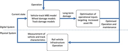
Predictive maintenance, where specific maintenance actions are predicted from historical data or vehicle-track multibody dynamics simulations (MBS), is arguably the most practical way of optimising the critical components necessitating maintenance. It is typically done in an asynchronous way. In the last decade, however, Digital Twins (DT) have come up as a powerful tool to monitor and predict the behavior of technical systems. DTs are a mathematical representation of assets in a validated model, which implies a need for a coupling between the actual asset and the model, i.e. sensors that monitor the important characteristics and a continuous or semi-continuous communication between the asset and the model. The DT could then be defined as synchronous simulation-based predictive maintenance model, where the maintenance limits are constantly re-calculated with actual operational and performance data from the asset (Figure 1).

Figure 1. Ideal configuration of a railway Digital Twin in the context of long-term damage monitoring and optimisation.

Coupling the topics predictive maintenance and condition monitoring with modelling and simulation of damage and Digital Twins is thus a promising area where minimal research has been carried out in the railway sector. Onboard Condition Monitoring (OCM) for improved diagnostics is a booming area in rail vehicles, driven by the technology leap that the electrification and increased computational power of other means of transport has brought. An example of feature extraction for OCM systems in freight vehicles can be found in [2]. Regarding predictive maintenance, there is a good theoretical body of knowledge around the actual processes and its coupling to the railway system in different contexts [3–6]. Additionally, the overlap of OCM with predictive and preventive maintenance is evident, with publications that treat them entwined as a common area [7].

The main challenge continues to be the accurate and robust modelling of damage evolution on wheels and rails, where the prediction of uniform wear [8–10] and Rolling Contact Fatigue (RCF) [11,12] in the meso-scale is one of the most recurring aspects. For the sake of conciseness, the more technical publications dealing with contact mechanics and tribology in micro- and nano-scales are not addressed, nor the extensive body of knowledge on track geometry degradation. In the end, to advance towards useful Digital Twins in the Railway sector, it is of utmost importance to have precise models of the railway assets in the wheel and rail damage simulations carried out, as DTs are essentially synchronous versions of Predictive Maintenance models.

This paper presents the methods developed for predicting both wheel and rail life based on RCF damage accumulation, discussing their accuracy and complexity levels. Two study cases are presented, one for wheel maintenance and a second one for rail maintenance, both for the Swedish Iron-Ore line.

Modelling of wheel and rail life

Wheel and rail life depends on many factors, which are related, as they share the contact interface, but not necessarily the same. To start with the definition of ‘life’ is the same for both: time from one maintenance action until the next one. For wheels, it is the mileage the wheelset ran before the maintenance action, while for a certain track section it is the number of gross tonnes (MGT) that rolled over that specific section. This circles back to the same concept for both sides again, as it refers to a certain number of load cycles in both cases.

In practice, wheels are reprofiled for different damaged conditions, which mostly refer to unsuitable profile shapes for the components in contact (uniform wear), rolling contact fatigue cracks (RCF), and local damages due to poor braking behaviour (wheel flats). For the infrastructure, rail grinding is performed due to similar reasons: unsuitable profiles, surface cracks, or local defects.

Damage models

The first step for a life prediction methodology is to model the damages present in the assets. For this, both RCF and Uniform Wear are simulated, to be able to predict their trend and find the operational limit of the assets. Limits for wear are classified in standards such as the Swedish standard SS-EN15313:2016, but the topic is more complex for RCF, and defining both a more detailed classification and reprofiling limits is still in progress. In literature, one can find different levels of precision for modelling RCF, from very precise solid mechanics or FEM techniques to qualitative crack initiation triggers based on the shakedown diagram [11].

The proposed RCF life calculation method is based on the use of output from multibody simulations (MBS) in order to calculate local instances of ratchetting in the contact patch, which is the principal contributor to RCF [13]. Ratchetting is a phenomenon where material subjected to cyclic loading undergoes a cyclic ‘creep’ deformation, i.e. a small and slow plastic deformation. Ratchetting does not always occur in conditions above the material’s yield limit. In fact, after the first few cycles the material gets hardened and with the help of residual stresses the response of the material could be totally elastic. This behaviour of the material is called Shakedown since the material shakes down to a lower state of deformation. The only thing contributing to RCF crack onset is the shear stress difference between the ratchetting instance and the shakedown limit, hereby called Shakedown-stress. Therefore, in this model, the Shakedown-stress is accumulated throughout the total running distance, and the RCF crack onset can be directly linked to this accumulation.

Damage modelling framework

The iterative method for damage calculations used in many wear-related research works [8] is used in this study to provide validity for both wheel and rail damage analyses. In each iterative step the accumulated wear and RCF is calculated and applied on the profiles so that next iteration simulations start with a partially damaged profile. The iterations continue until the desired simulation limits are achieved, which are case dependant. The final output is a predicted trigger for a maintenance action due to excessive RCF or wear, which can be a certain running mileage before the wheel profiles need to be reprofiled, or a certain number of axle tonnage passes before the rails need to be grinded out, depending on the study case.

Wear is calculated using Archard’s method, see [14]. It is a local method, meaning that the distribution of tangential stresses and slip velocities over the contact patch needs to be determined to calculate the wear accordingly.

• For wheel wear, the calculated wear for each patch in every wheel turn is integrated in the longitudinal direction along the simulated running distance, obtaining the wear depth as a function of lateral wheel coordinate for a given distance.

• For rail wear, one track section is analyzed where different wheelset passages are simulated. The effect of each passage is then accumulated in the same way as for wheels, obtaining a profile evolution for a given number of MGT.

For Rolling Contact Fatigue prediction, in analogy to wear calculation, the shear stresses are calculated within the contact patch, and the Shakedown-stresses are checked for each local mesh element and are then accumulated for the running distance in order to have a global measure for RCF.

Finally, the interaction between wear and fatigue needs to be addressed, as a heavily worn-out profile usually does not have time to develop fatigue cracks before the material is removed. Since crack propagation is not simulated, there is no need for complex interaction models between wear and RCF, so Burstow’s fatigue life model concept is used [12]. In this model, fatigue life is calculated as a function of the energy dissipation in the contact patch, Tγ. If the simulated energy dissipation is higher than the threshold $\overline{E_2}$, it is assumed that wear is completely governing the situation and there are no cracks propagating, which in practice means that the corresponding shakedown-stresses will be zero.

The thresholds are calculated by the material properties of the rail/wheel (1) $\overline{E_i}=\frac{{\nu }_{i}A}{2\sqrt{3}}({\sigma }_y+{\sigma }_U),\text{ for }i=1,2\mathrm{\&}3$(1) where, σ_y and σ_U are material yield limit and its ultimate tensile strength respectively and the corresponding suggested creepages v_i are 0.1%, 0.3% and 1%, see also [15]. Energy dissipation is then locally calculated for each mesh of the contact patch as: (2) $E(x,y)=q_x(x,y)({\nu }_x-\varphi y)+q_y(x,y)({\nu }_y+\varphi Nx)$(2) where, x and y are the profile coordinates, q_x and q_y are the tangential stresses in x and y direction respectively, and v_x, v_y and φ are the longitudinal, lateral and spin creepage.

This modelling allows for local calculation of the interaction in the contact patch before accumulating the Shakedown-stress, efficiently integrating both damage modes for the simulation.

Life limit

The life limit for a specific asset depends on the dominant damage mode, in the case of predictions using dynamic simulations, uniform wear or rolling contact fatigue. For wear simulations, where the actual profile evolution is simulated, these limits are easy to quantify based on existing rules and regulations. Life limits for RCF are not that straightforward to quantify, though. From a practical point of view, it is the instance when the fatigue cracks become problematic enough for needing removal. This is a qualitative measure that comes from experience, which makes the modelling system-dependant on an initial need for calibration against real conditions.

From a modelling perspective, the calculated Shakedown-stresses are accumulated at each load cycle, depending on the simulated asset: for wheel RCF this would mean each wheel revolution along the simulated running distance, while for rail RCF it means each wheel passage in a specific track section. When the wheel mileage or the amount of MGT leading to failure is known from the field studies, the shakedown-stress threshold to reach that failure limit will also be known from the simulations. This knowledge can then be used for sensitivity studies in that very same system, i.e. to predict the sensitivity of maintenance intervals with changes in operation such as lubrication condition, track gauge, loading, etc.

The resulting methodology is a low-complexity approach to RCF modelling, grounded in the physical fatigue behavior of wheel and rail materials, with system-specific empirical calibration. It allows the creation of specific tools for predictive maintenance management that can be integrated in future Digital Twin applications for railway systems due to their low complexity.

Study case: Swedish Iron-Ore line

To demonstrate the potential of the methodology, two different analyses are showcased for the Malmbanan, the Swedish Iron-Ore line. The line is mainly operated by heavy-haul ore freight trains operated by LKAB traveling between the mining sites in Kiruna and the ports of Narvik in Norway and Luleå in Sweden. For this study, traffic is composed by 10 fully loaded trains with 30 tonnes of axle load per day departing from Kiruna to Narvik, 2 of them with exceptional axle load of 32.5 tonnes, and the respective empty travel back from Narvik to Kiruna.

For the dynamic analyses, the multibody simulation model for the locomotive was provided by Bombardier Transportation (now Alstom) and Iron-Ore wagons are modelled according to [16]. Track related information is provided by the Swedish transport administration (Trafikverket) while the operational data is provided by LKAB. Additionally, the results of a five-years field study conducted by Ekberg [17] are used to tune the different parameters of the model.

The studied cases are, the analysis of wheel life for the locomotives, and the analysis of rail life for gauge widening scenarios.

Wheel life prediction for locomotives

This section showcases the use of dynamics simulations to predict maintenance (wheel reprofiling) intervals for the LKAB Iron-Ore locomotives. The goal of the model is to predict after how many kilometres of running distance the wheel profiles should be turned due to excessive RCF or severely worn profiles. The case follows the damage modelling framework, performing iterative time domain simulations equivalent to one return trip from Kiruna to Narvik for a total journey distance of 170 km. In each iteration the accumulated wear and RCF is calculated and applied on the wheel profiles so that in the next iteration simulations start with the partially damaged wheel profiles.

The final stage of the methodology is the comparison of the simulation results with field studies, which leads to a mathematical model coupling the dynamic behaviour with a specific maintenance limit. Each of these stages is briefly described in the following sections.

Simulation setup

The simulations are performed in the MBS software GENSYS [18]. Simulation outputs are quite sensitive to the modelling of the vehicle and operational conditions, especially those related to the wheel-rail contact. To increase the precision, different variables are handled in different ways. For instance, the vehicle speed is determined depending on the curve radius and super-elevation of each simulated track section according to the Swedish BVF 586.41 standard. In practice, the measured speed profiles of the locomotives show that the actual speed is somewhat fluctuating around these standard values, so to better represent the driving behaviour, the speed is chosen stochastically with small deviations from the calculated standard values. Other inputs are modelled as follows:

• Traction and braking

Braking and acceleration effort is taken from measurement data provided by LKAB. It is modelled as a longitudinal force applied at the buffer height of the rear of the locomotive, and a PID controller that calculates and applies the required torque on the wheelsets to keep the vehicle speed constant.

Most braking effort is provided by Electrodynamic Brakes in the locomotive, with only 5% of the braking covered by the friction brakes in the wagons. Therefore, the effect of block brake wear on the wheel profiles is neglected in this study.

The train travels loaded downhill from Kiruna to the port of Narvik and drives back empty and uphill to the mines in Kiruna. The differences in the traction and braking efforts are considered in the simulations and in every iteration step, changing both track geometry and the traction-braking efforts accordingly.

• Track sections

To avoid performing 170km-long time-domain simulations, an equivalent ‘load-collective’ representative of the track is used instead. This representative distribution covers other inputs such as wheel-rail friction level and vehicle speed. After analysing the geometry of the line, nine track sections are chosen for this study, as function of curve radius. The first curve category has all the sections with radii smaller than 350 m while, the largest curves are in the category where the curve radii are between 1300 m to 1500 m. All the track sections with larger radius than 1500 m are considered as straight line, since the vehicle speed is very low with a maximum of 70 km/h for empty cases. For all the simulation cases measured track geometry and irregularities are used. Simulations are set in way that eventually the train experiences all the measured track data. This is since that in each simulation case throughout the wheels life track sections are stochastically varied within each curve category. The measured track data includes the track geometry: longitudinal position on the track, superelevation (radian), vertical position of the centre of the track and the curvature of the section and the track irregularities: lateral, vertical, cant and gauge irregularities. The complete method has been thoroughly described in [19].

To increase the precision of the data, the line geometry and the corresponding irregularities are taken from measured data, cut into sections, and classified according to their curve radii. In each ‘wear-step’ one of these measured sections is chosen for each of the nine curve intervals. After choosing different sections in different wear-steps, a much more realistic track is simulated, compared to the previous procedure where an average section was simulated in each wear-step.

• Wheel-rail friction

In this study the friction coefficient is chosen stochastically for each track section within each wear-step using a normally distributed probability function around $\mu =0.4$. The mean value of the normal distribution is changed for sensitivity analyses, to analyse the effect of friction on the wheel life.

Locomotives are equipped with a flange lubrication device. In the simulations, the friction level drops to $\mu =0.15$ whenever there is flange contact. The transition of friction values from the tread to the flange is a linear interpolation within two centimetres at the flange root.

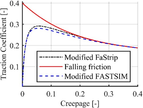
Falling friction has been implemented in the form of an advanced wheel-rail contact model. Dynamic simulations are performed using a built in MBS module based on [20], but in the post processing stage the FaStrip algorithm is applied instead of FASTSIM [21]. There is negligible difference between the two methodologies when estimating the creep forces, but FaStrip substantially improves the accuracy of the shear stress estimation [22]. Figure 2 shows the effect of falling (dynamic) friction on creep forces at high creepages.

• Wheel and rail profiles

Figure 2. Behaviour of the modified FASTSIM and FaStrip algorithms in high pure longitudinal creepages.

At the Iron-Ore line, different pairs of rail profiles are applied depending on the curve radii [12]. The same logic is followed in the simulations, see Table 1. The rail profile shapes are obtained from averaging the measured rail profiles along the corresponding track section, see Figure 3.

Figure 3. Rail profiles used in Iron-Ore line.

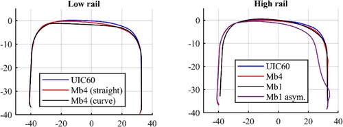
Table 1. Rail profiles distribution in Iron-Ore line.

	High rail	Low rail
Ri ≤ 600 m (Norway)	MB1 asymmetric	MB4
Ri ≤ 600 m (Sweden)	MB1	MB4
Ri > 600m	MB1	UIC60
Straight track	MB4 & UIC60	MB4 & UIC60

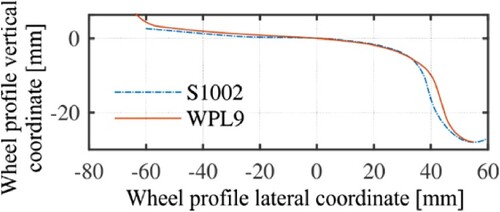
For the wheel profiles, the nominal profile for the Iron-Ore line is used, WPL9, see Figure 4 for a comparison with the standard S1002 profile.

Figure 4. Locomotive wheel profile against the standard wheel profile S1002.

Damage calculation

Wear and RCF is calculated following the methodology described in section 2. Due to the particularities of wheel damage modelling, a more specific description follows.

For uniform wear prediction, wear is simulated at the contact patch in every wheel turn for the whole running distance. It is then integrated longitudinally; the total wear depth can be obtained corresponding to the simulation distance as a function of lateral wheel coordinate (Figure 5). This method was first presented in [8] and has been successfully applied in many research works afterwards.

Figure 5. Schematic picture summation of the wear per strip at each contact patch in every wheel revolution to give total wear depth. The horizontal axis is the direction of rolling on the rail, the lateral axis is lateral coordinate of the wheel profile [19].

The results are shown in Figure 6, where flange height and flange thickness development as a function of running distance are depicted. A very good agreement with measured worn profiles can be observed.

Figure 6. Development of flange height and thickness due to wear as function of running distance; comparison between the simulations and measurement [19].

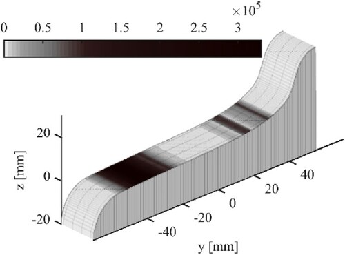
RCF damages are also modelled as described in the methodology section, including the effect of wear in crack development. Figure 7 shows the number of wheel rotations with positive shakedown-stress after 50,000 km of simulated running distance. Note that to show the worst-case scenario, only the accumulated damage of the first wheelset is shown (averaged between the left and the right wheel). These numbers are modified with a correction, see Eq. 1(1) $\overline{E_i}=\frac{{\nu }_{i}A}{2\sqrt{3}}({\sigma }_y+{\sigma }_U),\text{ for }i=1,2\mathrm{\&}3$(1) . The main affected wheel area, which is between −20 and −45 mm, coincides well with the field observations reported in [17] on the field side of the wheel.

Figure 7. RCF-number (Nr) after around 50,000 km simulated running distance; Leading inner wheel.

Wheel life prediction

According to [17] the median of the running distance intervals between two consecutive wheel reprofiling due to RCF cracks for the locomotives is around 40,000 km, while the maximum is around 70,000 km. Therefore, iterations are continued until 70,000 km of simulated running distance is reached, corresponding to around 400 wear-steps and 3,600 time-domain simulations for each of the studied cases. Each wear-step iteration takes around 20 minutes real world time, so the number of case studies and the simulated running distance are limited to six different cases, making the total number of time domain dynamics simulations about 21,000.

The simulation results of accumulated shakedown-stresses for all cases are shown in Figure 8 (left), covering three different friction values, a non-lubricated case, a reduced rolling radius case (min D), and a non-ED braking case (NoED). The nominal case is the one with friction level 0.4. Note that friction levels 0.3, 0.4 and 0.5 refer to the nominal value of the static friction of the wheel tread. Due to the flange lubrication system the friction levels at the flange are assumed to be 0.15. The friction values are chosen stochastically with a normal distribution around these nominal values. The case with no lubrication is when the flange lubrication is turned off and both tread and flange have the same friction values. As can be seen in Figure 8, the trends are almost linear, so a linear extrapolation would be a good estimation to predict the shakedown-stresses at larger running distances.

Figure 8. Cumulative shakedown-stresses (left) and the corresponding expected wheel life (right).

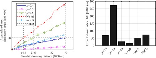
Case min D studies the effect of wheel radius on the limit of the wheel life, where simulations are performed with the minimum allowed wheel radius of 575 mm rather than the nominal radius of 625 mm. This case is interesting because in many cases locomotives operate on wheels with a diameter smaller than their nominal one, as they reach their reprofiling limit quite soon and need to be turned quite often. Finally, in the case with no electrodynamic braking (NoED) it is assumed that all the braking efforts are handled by the wagons, so the locomotive wheels are not affected by braking-related creepages.

For the wheel life calibration step, cumulative maximum shakedown-stresses are compared for all the cases with the reference case at its maximum life of 70,000 km, obtaining the predicted maximum wheel life for every case, see Figure 8 (right). As can be seen in the figure, decreasing the average friction coefficient by 0.1 point significantly increases wheel life and, on the contrary, increasing it by 0.1 point shortens the wheel lives even further. The case with minimum wheel life is the one without flange lubrication, which is probably the reason that RCF cracks and short reprofiling intervals occur way more often in wintertime, when the lubrication system does not function properly due to the cold artic climate.

Decreased wheel radius slightly shortens the wheel life and turning off the ED braking does not have any significant effect on the wheel life, which is experienced in the field studies conducted by LKAB too.

Rail life

At the Iron-Ore line, soon after a track upgrade in 2004, an increase in rolling contact fatigue (RCF) related damage appeared in the form of head checking on the high rail in curves. Nowadays, the head checking damage is under control thanks to the change of the existing profile to a new wear-adapted rail profile, MB1, created by relieving the gauge corner of the nominal UIC60E1 rail profile (see Figure 3), improving the damage situation [23]. Here ‘under control’ means that the depth of RCF cracks after each grinding campaign is less than a millimetre. Note that grinding is performed every six months for tight curves in which the depth of grinding is around 0.2 mm minimum distance between the ground nominal profile and the worn profile. Later an optimized wear adapted profile was introduced, the so called MB4, proving their efficiency as the damage on the rail has been reduced and thus the overall necessary maintenance.

In addition to this, another wear adapted rail profile with the objective of solving the low rail RCF called MB5 has been created. This profile is 0.4 mm higher in the field side than the UIC60E1, which induces a wider contact band, somewhat relieving the RCF problems. It was found though that this profile, although beneficial to the low rail, actually aided the forming of RCF damage on the high rail [23]. This profile is still experimental, as part of the investigative efforts to control the degradation rate of the rails on the Iron-Ore line. Thus, the profile is not used in the simulations.

Whilst the head checking issues could be resolved using a wear adapted rail profile and planned grinding campaigns, the low rail damage remains a problem. As it is reported in [23], there was still a problem with RCF spalling on the low rail of curves with a radius below 650 m (see Figure 9). A study of the track parameters was carried out, pointing to a widened gauge as the common factor: damage appeared for gauges wider than 1450 mm. The widened gauge creates a limited band towards the field side where the contact points are concentrated, developing rail surface cracks that grow deep enough so that they are no longer removed during rail grinding operations.

Figure 9. Left: concentrated contact on low rail with wide gauge, Right: spalling along centre-line of low rail [23].

The aim of this simulation case is to predict the damage on the low rail of small radius curves, and to better understand how the gauge width affects the risk of surface initiated rolling contact fatigue.

Simulation setup

MBS simulations include the vehicle models for both locomotive and wagons for a set of curves with different characteristics. The northern loop of the Iron-Ore line has a total of 113 curves with a radius below 750 m, so a selection of five curves is made, one in each 50 m interval from 500-750 m, as a representative for the interval (see Table 2).

Table 2. Curve selection with their respective curve radii, location on the line and cant deficiency.

Radius [m]	Start km	End km	Cant deficiency [mm]
508	122.216	122.689	−11.2
594	78.086	78.446	−1.3
621	61.930	62.105	−21.3
683	13.735	14.155	1.3
724	47.153	47.313	7.4

Operational data is as described in previous sections, with a spread of loading cases for the locomotive and wagon influence in the total simulation cases. Note that the weight of the locomotive is unchanged regardless of the weight of the wagons in which the axle load is always 30t while for the wagon 10% of the time the axle load is 32.5t, 40% of the time the axle load is 30t and the rest of 50% the wagon is empty and the axle load is 5t.

In each curve simulation, many other simulation variables and parameters have either deterministic or stochastic distributions that can be modelled. For example, the distribution of loads on the vehicles is known from the traffic schedule, but friction in the wheel-rail contact is not fully known so it is represented with normally distributed stochastic values centred around a nominal value. Figure 10 contains a summary of all the individual parameters used in the simulations, and a combination of all these parameters is used for each individual damage prediction simulation, weighting their relative contribution to the total damage according to their relative importance.

Figure 10. Summary of all parameters included in the simulations.

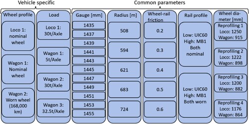
The effect of friction, wheel/rail characteristics, and load must be scaled with the expected traffic for one wear period. This period can for example be a specific season or the time between rail grindings. In the current work the time which it takes until the cracks appear on the low rails is considered for the simulations, i.e. 3.5 months. The equally distributed parameters in the model are wheel and rail diameters/profiles. These are assumed to be equally likely to appear in traffic, yielding a scaling factor pd = 0.25 for each wheel diameter and pr = 0.5 for each rail profile. For the locomotives only the nominal wheel profiles are used in the simulations. However, for the wagon one additional parameter is considered, namely the wheel profile, as both a new and a worn one is used, yielding ps = 0.5, with both alternatives equally probable.

Rail life prediction

To calibrate the simulation results, a more detailed analysis of a certain section of the line is performed, to identify locations with the risk of RCF on the rail surface. The section is a left-hand curve with radius of 508 m between Vassijaure and Riksgränsen. The rail profile and track gauge were measured in May of 2019, with only a few weeks between them. At that time, the track gauge in the reference curve was 1447 mm.

The expected time it takes for rolling contact fatigue to appear on the rail was determined from discussions with maintenance engineers. After a period of 3.5 months, or 105 days clear signs of RCF can be seen on the rails. Given the schedule of the vehicles running on the track, gross ton passing can be determined, which is then directly linked to the Shakedown limit based on the output from the MBS simulations.

This threshold shear stress level is used for all simulation cases, each of them having their own track characteristics (track gauge, irregularities, rail profiles …). The traffic scaling is done with the same variables as the rest of the simulations. The limit values for the low rail using the MGT of axle passes is 0.357 and accumulated maximum shear stress above the shear strength of the rail is 7,430,000. The validation case then, provides a reference damage accumulation value for the other simulations.

Additionally, it provides an opportunity to study how well the predicted damage contact band aligns with visual inspections. By plotting the location of the contact points with RCF, one can identify where on the rail the contact band lies. Comparing this plot with a photograph it will be possible to check for the agreement between simulation and field results.

Full scale investigation

Figures 11 and 12 show the results for the five studied curves. The figures depict the 105-day accumulated shear stress for different track gauges, weighted with the traffic running through the section; the loading cases are respectively fully laden wagons (30 tons/axle, blue), extra laden wagons (32.5 tons/axle, red) and empty wagons (5 tons/axle, yellow). The black horizontal line represents the limit value. The right plot depicts the values of each case at each gauge, to enable an easier comparison of the relative importance of the different loading conditions.

Figure 11. Accumulated shear stress above the shear yield limit in 3.5 months traffic on the low rail [MPa] vs Track gauge [mm] at Curve 1, R508 m, Cant deficiency −11.2 mm, L = locomotive, W = wagon.

Figure 12. Accumulated shear stress above the shear yield limit in 3.5 months traffic on the low rail [MPa] vs Track gauge [mm] at Curve 3, L = locomotive, W = wagon; (a) R594 m, (b) R621 m, (c) R683 m and (d) R724 m.

Figure 11, Accumulated shear stress above the shear yield limit in 3.5 months traffic on the low rail [MPa] vs Track gauge [mm] at Curve 1, R508 m, Cant deficiency −11.2 mm, L = locomotive, W = wagon.

The results show a similar behaviour for all curves, with a rather stable behaviour at lower gauge widths, and a progressive non-linear increase for gauges higher than approx. 1445 mm. It is noteworthy that the wagons running empty have a larger number of load cases with RCF at any given track gauge. There is a clear trend that the loaded and unloaded trains at each gauge are very close together (only considering the loaded trains at 30 t axle load). There is a large difference between the trains running at 30t and 32.5t axle load, which is due to the different amount of vehicles running, which gives a lower overall accumulated damage for the small amount of trains with 32.5 t axle load.

The results show a similar behaviour for all curves, with a rather stable behaviour at lower gauge widths, and a progressive non-linear increase for gauges higher than approx. 1445 mm. It is noteworthy that the wagons running empty have a larger number of load cases with RCF at any given track gauge. There is a clear trend that the loaded and unloaded trains at each gauge are very close together (only considering the loaded trains at 30 t axle load). There is a large difference between the trains running at 30t and 32.5t axle load, which is due to the different amount of vehicles running, which gives a lower overall accumulated damage for the small amount of trains with 32.5 t axle load.

The main differences between the different curves are the total amount of damage accumulation. For curves 1–3 the widest gauges accumulate damage to an extent well over the allowed maximum limit. For Curves 4 and 5 the trend is similar, but the damage accumulation is always below the allowed limit.

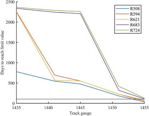
Figure 13 depicts the results for the five curve cases, in terms of how many days it takes to reach the limit value calculated in the validation case for five of the track gauges simulated. This figure highlights the dramatic change in life expectancy of the rails between two consecutive gauges, indicating that maintenance limits can not only be very sensitive to curve radius but also track widening. As discussed in previous sections, the wheel-rail contact position is what determines if there will be a concentration of highly stressed contact bands where damage is accumulated. For gauges above 1450 mm, all curve radii have a similar behaviour and thus a significantly reduced asset life.

Figure 13. Number of days to reach the damage limit at five track gauges (1435, 1441, 1445 mm, 1451 mm&1455 mm), for each of the five curving cases.

Rail damage contact bands

In Figure 14, the location of the rail RCF damage for different track gauges after 105 days is depicted. This type of plot allows for an overview of where damage can be expected depending on the current gauge width on the line. The damage concentration is the highest at the centre of the rail for all gauges, with a substantial damage increase for track gauges above 1445 mm. There is a good visual agreement between simulations and real-life experience (see Figure 14). As it is seen in the figure, the top of rail in the simulation plot lies around the −5 mm point, which corresponds to the lower edge of the contact band in the photo of the rail.

Figure 14. Comparison between simulated damage points on the low rail in curve 1 with actual damage on the rail; Simulated results of curve 1 with R = 508 m (left); brighter colour indicates more load cases with RCF (X-axis: Track gauge [mm], Y-axis: Lateral position[mm]), Actual rail photo taken 2020 (right).

Conclusions and further work

A methodology for the simulation of asset life has been developed that allows for estimating the expected changes in wheel or rail life when different adjustments are made in the railway system, the operation or if environmental parameters change. The method combines previous state of the art simulation techniques with a newly developed fatigue life calculation method to build the framework. Given the extreme variety of parameter combinations, after an initial calibration this methodology allows to analyse the influence of different parameters in the asset life in an automated way, enabling a fast and resource-light analysis of system-level changes.

The methodology has been applied to the Iron-Ore line in northern Sweden. First, life of locomotive wheels has been determined and its variation with different operational and environmental variables has been studied, such as stochastic friction values in the wheel-rail contact or the influence of wheel diameter on RCF generation, but also deterministic variables such as the use of electrodynamic braking.

The second case study calculates rail damage, specifically the effect of gauge widening on the expected rail life. The analysis also covers the experimental validation of the damages with respect to contact bands for different curve radii.

The studied cases show the capabilities of the model for understanding how specific changes in operational, physical, or environmental variables influence the operational life of important and costly assets such as wheels and rails. The relatively low computational effort makes its use straightforward in predictive maintenance. Its usage for synchronous Digital Twin applications in the Railway sector would be enabled by advances in the use of onboard or trackside condition monitoring.

Disclosure statement

No potential conflict of interest was reported by the author(s).

References

- European Comission. “Roadmap to a Single European Transport Area – Towards a competitive and resource efficient transport system,” White Paper COM(2011) 144 final, Mar. 2011.
- Gericke C, Hecht M. CargoCBM – Feature Generation and Classification for a Condition Monitoring System for Freight Wagons. J Phys Conf Ser. 2012;364:0012003. doi:10.1088/1742-6596/364/1/012003.
- Villarejo R, Johansson C-A, Galar D, et al. Context-driven decisions for railway maintenance. Proceedings of the Institution of Mechanical Engineers, Part F: Journal of Rail and Rapid Transit. 2016;230(5):1469–1483. doi:10.1177/0954409715607904.
- Ciocoiu L, Siemieniuch CE, Hubbard E-M. From preventative to predictive maintenance: The organisational challenge. Proceedings of the Institution of Mechanical Engineers, Part F: Journal of Rail and Rapid Transit. 2017;231(10):1174–1185. doi:10.1177/0954409717701785.
- Higgins C, Liu X. Modeling of track geometry degradation and decisions on safety and maintenance: A literature review and possible future research directions. Proceedings of the Institution of Mechanical Engineers, Part F: Journal of Rail and Rapid Transit. 2018;232(5):1385–1397. doi:10.1177/0954409717721870.
- Zhu W, Yang D, Huang J. A hybrid optimization strategy for the maintenance of the wheels of metro vehicles: Vehicle turning, wheel re-profiling, and multi-template use. Proceedings of the Institution of Mechanical Engineers, Part F: Journal of Rail and Rapid Transit. 2018;232(3):832–841. doi:10.1177/0954409717695649.
- Zhang D, Hu H, Roberts C, et al. Developing a life cycle cost model for real-time condition monitoring in railways under uncertainty. Proceedings of the Institution of Mechanical Engineers, Part F: Journal of Rail and Rapid Transit. 2017;231(1):111–121. doi:10.1177/0954409715619453.
- Jendel T. Prediction of wheel profile wear—Comparisons with field measurements. Wear. 2002;253(1–2):89–99. doi:10.1016/S0043-1648(02)00087-X.
- Braghin F, Lewis R, Dwyer-Joyce RS, et al. A mathematical model to predict railway wheel profile evolution due to wear. Wear. 2006;261(11–12):1253–1264.
- Apezetxea IS, Perez X, Casanueva C, et al. New methodology for fast prediction of wheel wear evolution. Veh Syst Dyn. 2017;55(7):1071–1097. doi:10.1080/00423114.2017.1299870.
- Krishna VV, Hossein-Nia S, Casanueva C, et al. Rail RCF damage quantification and comparision for different damage models. Railway Engineering Science; 30(1):23–40.
- Hossein-Nia S, Sichani MS, Stichel S, et al. Wheel life prediction model – an alternative to the FASTSIM algorithm for RCF. Veh Syst Dyn. 2018;56(7):1051–1071. doi:10.1080/00423114.2017.1403636.
- Johnson KL. The Strength of Surfaces in Rolling Contact. Proceedings of the Institution of Mechanical Engineers, Part C: Mechanical Engineering Science. 1989;203(3):151–163. doi:10.1243/PIME_PROC_1989_203_100_02.
- Archard JF. Contact and Rubbing of Flat Surfaces. J Appl Phys. 1953;24(8):981), doi:10.1063/1.1721448.
- Spangenberg U, Fröhling RD, Els PS. Influence of wheel and rail profile shape on the initiation of rolling contact fatigue cracks at high axle loads. Veh Syst Dyn. 2016;54(5):638–652. doi:10.1080/00423114.2016.1150496.
- Hossein Nia S, Jönsson P-A, Stichel S, et al. “Investigation of Rolling Contact Fatigue on the wheels of a three-piece bogie on the Swedish Iron-Ore Line via multibody simulation considering extreme winter conditions,” In Proceedings of the international heavy haul conference, New Delhi, India, 2013, pp. 357–363.
- Ekberg A. “Iron-Ore line – Damage on loco wheels,” Chalmers University of Technology, Göteborg, Sweden, 20161214-LKAB-Lokhjul, 2016.
- Persson I. GENSYS.1312 Reference Manual,” DEsolver AB, 2013. [Online]. Available: gensys.se.
- Hossein Nia S, Casanueva C, Stichel S. Prediction of RCF and wear evolution of Iron-Ore locomotive wheels. Wear. 2015;62–72:62–72. doi:10.1016/j.wear.2015.05.015.
- Spiryagin M, Polach O, Cole C. Creep force modelling for rail traction vehicles based on the Fastsim algorithm. Veh Syst Dyn. 2013;51(11):1765–1783. doi:10.1080/00423114.2013.826370.
- Polach O. Creep forces in simulations of traction vehicles running on adhesion limit. Wear. 2005;258(7–8):992–1000. doi:10.1016/j.wear.2004.03.046.
- Sichani MS, Enblom R, Berg M. An alternative to FASTSIM for tangential solution of the wheel–rail contact. Veh Syst Dyn. 2016;54(6):748–764. doi:10.1080/00423114.2016.1156135.
- Asplund M, Famurewa SM, Schoech W. A Nordic heavy haul experience and best practices. Proceedings of the Institution of Mechanical Engineers, Part F: Journal of Rail and Rapid Transit. 2017;231(7):794–804. doi:10.1177/0954409717699468.