Can a nonlinear quasi-zero-stiffness spring improve the ride quality of a vehicle?

Abstract

The paper examines the possibility of using a nonlinear Quasi-Zero-Stiffness (QZS) spring in a vehicle suspension. The response of a Single Degree of Freedom (SDOF) model to harmonic base excitations is obtained which may be unstable and unbounded depending on the excitation level and the damping ratio. This is followed by obtaining the response of the SDOF model to harmonic base excitation with an amplitude that is varying according to a road profile spectrum. Such dependency of the excitation amplitude to the frequency changes the qualitative behaviour of the nonlinear system and the responses would be always bounded. The QZS spring also improves the isolation of the system. Transient responses of a quarter car model with a QZS suspension to a road hump and random road profile are investigated. The maximum acceleration of the vehicle with the QZS suspension passing over the speed hump is considerably lower than a vehicle with a conventional linear suspension. Wb weighted RMS of acceleration (BS 6841-1987) is also lower by as much as 14% for a vehicle with the QZS suspension travelling at 30 km/h on a class E road compared to its linear counterpart.

KEYWORDS:

• Nonlinear spring
• QZS spring
• quarter car model
• frequency response function
• road profile excitation
• speed hump

1. Introduction

A vehicle suspension should provide a high level of isolation from road surface disturbances. This is achieved via a relatively low stiffness spring in a conventional suspension. Reducing the stiffness would further improve the ride by providing better isolation from the road surface but it may adversely affect the vehicle handling as well as result in large static deformation, both unaffordable in road vehicles. A nonlinear spring may be used to overcome this problem by combining a high load-bearing capacity with a low stiffness when loaded for small disturbances. Such springs can be tuned to achieve a zero stiffness at the loaded position which is known as Quasi-Zero-Stiffness (QZS) [1]. The purpose of the current study is to examine the effect of road excitations on the response of a system with a QZS spring and to understand how a QZS spring can improve the ride quality of a vehicle via a simple model. The handling of such a vehicle is not investigated in this paper and requires more complex models.

The use of nonlinear springs for vibration isolation is studied extensively (e.g. see [2,3]). A QZS vibration isolator possesses very rich dynamics. Multiple stable and unstable solutions exist for such an isolator which can result in a jump phenomenon in the frequency response function [4,5]. The type of solution depends on the damping and excitation level and generally nonlinear dynamics would be attainable for a low level of damping. The application of nonlinear springs to the road vehicle was limited to a handful of studies.

Anubi et al. [6] introduced a variable stiffness suspension system using a combination of horizontal and vertical suspension struts and examined the performance of their design. The performance of the suspension system is studied numerically and test results for a drop test are provided. Saini [7] used a snap through negative stiffness spring using buckled beams to form a variable stiffness system. The beam possesses a force-deflection curve with a negative slope when snapping from a stable configuration to another one. They examined the characteristics of the system statically and used direct numerical integration to obtain the transmissibility of the proposed suspension and compared it with a linear one. He concluded the proposed nonlinear suspension can improve vibration transmissibility.

Li et al. [8] obtained the response of a single degree of freedom (SDOF) quarter car model with Duffing type stiffness and nonlinear damping to multi-harmonic road excitation. They showed for a certain parameter range the response of the system can be chaotic. Litak et al. considered the effect of the gravity force on the same system with softening nonlinearity in [9] and with a stochastic component added to the excitation in [10]. They showed that gravity break the symmetry in the potential and the response can be quasi-periodic, synchronised or chaotic for a large amplitude of excitation. Zhou et al. [11] obtained the response of a nonlinear suspension under harmonic excitation and studied the effect of different system parameters on the response. Zeng et al. [12] introduced a combination of a QZS spring, nonlinear energy sink and inerter for a vehicle suspension. They used a quarter car model to examine the response of the system and used Harmonic Balance Method and numerical integration to obtain the response of the system to constant amplitude harmonic excitation. They obtained the displacement and acceleration of the sprung mass and used the frequency response curve of the tyre force as a measure of handling. It is concluded that the new suspension improves the vehicle's ride and handling.

In the above studies, a constant amplitude harmonic base excitation is assumed in order to obtain the response of the nonlinear suspension. However, the road surface profile amplitude has a spatial frequency dependency [13]. In this paper, this dependency is considered and the response of a vehicle with a QZS suspension to road excitations is obtained. The paper is divided into two parts. In the first part, an SDOF model is used to derive an analytical solution to standard road excitations. The analysis serves as a basis for future studies and also for the second part of this paper where the transient response of the QZS suspension is examined. A 2DOF quarter car model is used to compare the response of a vehicle with conventional suspension travelling over a speed hump and to random road excitation in section 3. The paper finishes with discussions and conclusions.

2. Frequency response function of a SDOF system with a QZS spring

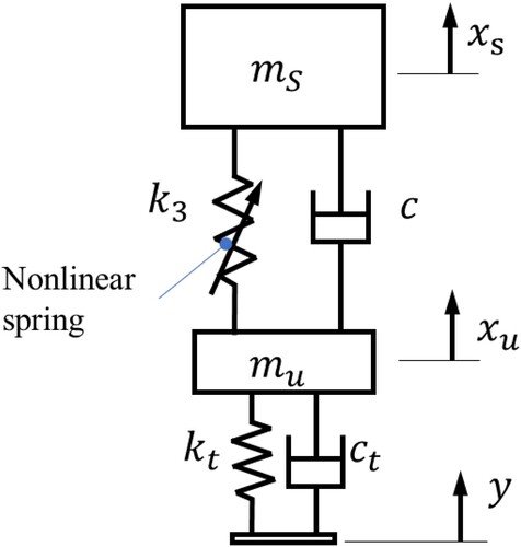
The constitutive equation of a QZS spring may be approximated by a third-order polynomial with a cubic term only [14]. This is the simplest form and a common approximation for a nonlinear spring with a QZS characteristic. The schematic of the SDOF with a QZS spring is shown in Figure 1. This is used in this section to obtain a closed-form solution for the frequency response function and obtain damping ratios that would result in qualitative changes in the response of the system.

Figure 1. The schematic of a single degree of freedom model with a nonlinear QZS spring.

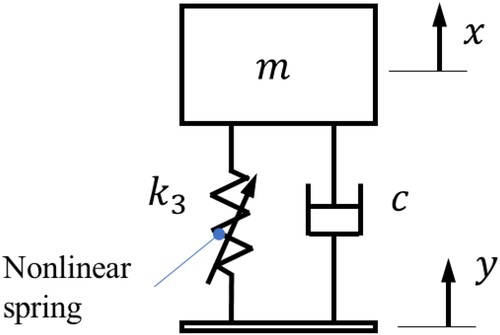
The equation of motion of the SDOF model shown in Figure 1 can be obtained in terms of relative displacement $z=x-y$, (1) $m\ddot{z}+c\dot{z}+k_3{z}^3=-m\ddot{y}$(1) where $m$ is the mass, $c$ is the damping coefficient, $k_3$ is the nonlinear stiffness coefficient, $x$ is the displacement of the mass measured from the static equilibrium position, and $y$ is the base excitation representing the road surface disturbances.

For a system with a linear spring, the stiffness term in Equation (1) should be replaced by $kz$ and the fundamental frequency of such a model would be ${\omega }_n=\sqrt{k/m}$. The static deformation of the mass due to its weight would be $\delta =g/{\omega }_n^2$. Equation (1) can be normalised using the linear system parameters which enables a direct comparison between the two systems, (2) ${\hat{z}}^{\mathrm{\prime }\mathrm{\prime }}+2\zeta {\hat{z}}^{\mathrm{\prime }}+\gamma {\hat{z}}^3=-{\hat{y}}^{\mathrm{\prime }\mathrm{\prime }}$(2) where $\hat{z}=z/\delta$ is nondimensional relative displacement, $\hat{y}=y/\delta$ is nondimensional road elevation, $\zeta =c/2m{\omega }_n$ is damping ratio, $\gamma =k_3{\delta }^2/k$ is nonlinear stiffness ratio and $\tau ={\omega }_{n}t$ is nondimensional time. The prime is used for differentiation with respect to nondimensional time, i.e. $(.{)}^{\mathrm{\prime }}=d(.)/d\tau$. If the static deformation of both nonlinear and linear systems are considered the same, the nondimensional nonlinear stiffness term would be equal to unity, i.e. $\gamma$ =  1 (for the nonlinear system $mg=k_3{\delta }^3$ and for the linear system $mg=k\delta )$. This is used as a nominal value for the nonlinear stiffness coefficient here, however, other values may be used due to the design or performance requirements. The Harmonic Balance Method is used to obtain the steady-state response of the system to the base excitation $y=Y\cos (\omega t)$. This is a special case of a nonlinear base exciting system that is studied in detail (for example look at [4,5,15]) and is provided here for completion. Equation (2) can be rewritten as, (3) ${\hat{z}}^{\mathrm{\prime }\mathrm{\prime }}+2\zeta {\hat{z}}^{\mathrm{\prime }}+\gamma {\hat{z}}^3=\hat{Y}{\mathrm{\Omega }}^2\cos (\mathrm{\Omega }\tau )$(3) where $\hat{Y}=Y/\delta$ is the nondimensional amplitude of the excitation and $\mathrm{\Omega }=\omega /{\omega }_n$ is the nondimensional frequency. By assuming a solution in the form of $\hat{z}=\hat{Z}\text{cos}(\mathrm{\Omega }\tau +\varphi )$, where $\hat{Z}$ is the nondimensional amplitude of the relative displacement and $\varphi$ is its phase, and neglecting the term including $\cos (3\mathrm{\Omega }\tau )$ the following equation can be obtained for $\hat{Z}$ and $\varphi$, (4) $\begin{array}{rl}\frac{3}{4}{\hat{Z}}^3\gamma -\hat{Z}{\mathrm{\Omega }}^2& =\hat{Y}{\mathrm{\Omega }}^2\cos (\varphi )\end{array}$(4) (5) $\begin{array}{rl}-2\zeta \mathrm{\Omega }\hat{Z}& =\hat{Y}{\mathrm{\Omega }}^2\sin (\varphi )\end{array}$(5)

Equations (4) and (5) can be squared and added to obtain a frequency–amplitude equation, (6) $({\hat{Z}}^2-{\hat{Y}}^2){\mathrm{\Omega }}^4+\left(4{\hat{Z}}^2{\zeta }^2-\frac{3{\hat{Z}}^4\gamma }{2}\right){\mathrm{\Omega }}^2+\frac{9{\hat{Z}}^6{\gamma }^2}{16}=0$(6)

Solving Equation (6) yields two solutions for $\mathrm{\Omega }$ as a function of amplitude $\hat{Z}$, (7) ${\mathrm{\Omega }}_{1,2}=\frac{1}{2}\sqrt{\frac{-3{\hat{Z}}^4\gamma +8{\hat{Z}}^2{\zeta }^2\mp \sqrt{9{\hat{Y}}^2{\hat{Z}}^6{\gamma }^2-48{\hat{Z}}^6\gamma {\zeta }^2+64{\hat{Z}}^4{\zeta }^4}}{{\hat{Y}}^2-{\hat{Z}}^2}}$(7)

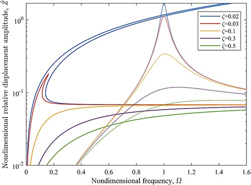
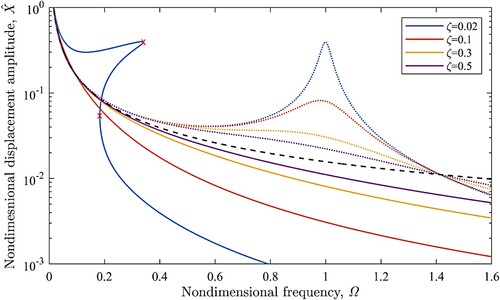
The frequency response curves for a base amplitude of $\hat{Y}=0.068$ is shown in Figure 2. The nondimensional excitation amplitude is derived by assuming an amplitude of excitation of $Y=1$ cm for a vehicle with a fundamental frequency of 1.3 Hz, i.e. $\delta =0.147$ m. Depending on the damping ratio, nonlinear coefficient and excitation amplitude, three different types of solution can be observed. For a moderate value of damping ratio, Equation (7) possesses two real solutions which are resonant and non-resonant branches of the frequency response curve of the system [4,5,15]. The response of the system for a damping ratio of $\zeta =0.03$ in Figure 2 is an example of such a response. The maximum amplitude can be approximated by the point where resonant and non-resonant branches meet, which can be obtained by setting the inner radicand in Equation (7) equal to zero, (8) ${\hat{Z}}_{\text{max}}=\frac{8{\zeta }^2}{\sqrt{3}\sqrt{-3{\hat{Y}}^2{\gamma }^2+16\gamma {\zeta }^2}}$(8)

Figure 2. The frequency response curve of the relative displacement amplitude of the SDOF system for a constant amplitude of excitation and different damping ratios, $\gamma =1$ and $\hat{Y}=0.068$; solid line: QZS spring, dotted lines: linear spring.

The solution for ${\hat{Z}}_{\text{max}}$ can be substituted in Equation (7) to obtain its corresponding frequency, (9) ${\mathrm{\Omega }}_{\text{max}}=8\sqrt{2}\sqrt{-\frac{{\zeta }^6}{9{\hat{Y}}^4{\gamma }^2-72{\hat{Y}}^2\gamma {\zeta }^2+128{\zeta }^4}}$(9)

The radicands of Equations (8) and (9) should be positive in order to have a real value for the maximum amplitude and its corresponding frequency which provides the range for the damping ratio in which a resonant and nonresonant branch exists, i.e. $\sqrt{3\gamma }\hat{Y}/4<\zeta <\sqrt{3\gamma }\hat{Y}/\sqrt{8}$.

For low values of damping, $\zeta \le \sqrt{3\gamma }\hat{Y}/4$, there would be no real solution for Equation (8), and the response would be of a hardening type and unbounded. An example of such frequency response curves is shown in Figure 2 for a damping ratio of 0.02.

By increasing the damping ratio the system behaves similarly to a highly damped linear system and there would be no multiple solutions (bend) in the frequency response curve and the peak vanishes by increasing the damping further. For damping ratios $\ge$ $\sqrt{3\gamma }\hat{Y}/\sqrt{8}$, the radicand of Equation (9) would be negative and the resonant branch seizes to exist. The response is similar to the response of an overdamped linear system for this range of damping.

The response of an equivalent system with a linear spring is shown with the dotted lines in Figure 2. For the excitation amplitude of this case, the amplitude of the peak when it is bounded is much smaller for the QZS system and occurs at lower frequencies, e.g. compare the response of the linear system with the QZS system for $\zeta =0.03$. Furthermore, for specific values that are used here, the peak in the frequency response curve of the QZS system disappears for a lower value of damping ratio than that for the linear system, for example, there is a peak in the frequency response curve of the linear system for $\zeta =0.1$ and $0.3$ while there is no peak in the response curve of the QZS system for the same damping ratios. By increasing the amplitude of excitation, the peak frequency would shift to the higher frequencies and the amplitude of the peak for the QZS system can be larger than the linear system. This necessitates obtaining the response of the system to road excitations.

In the above analysis, the amplitude of displacement for the base excitation is assumed constant over the frequency range of interest. However, the Power Spectral Density (PSD) of the road elevation profile is not constant and has an inverse relation with the wavenumber [13]. The standardised road profile can be used to obtain harmonic excitations with an amplitude that is changing in a similar way to a road profile spectrum. The frequency response curve of the system can be obtained using these excitation amplitudes. International standard ISO 8608:2016 [13] has categorised roads into different classes, A to H, where A is the smoothest road surface. The power spectral density of each class can be obtained using the standard formula, (10) $G_d(\overline{\mathrm{\Omega }})=G_d({\overline{\mathrm{\Omega }}}_0){\left(\frac{\overline{\mathrm{\Omega }}}{{\overline{\mathrm{\Omega }}}_0}\right)}^{-w}$(10) where $G_d$ is the displacement PSD, $\overline{\mathrm{\Omega }}$ is angular spatial frequency, ${\overline{\mathrm{\Omega }}}_0=1$ rad/m is the reference angular spatial frequency and $w=2$ is the exponent of the PSD for standardised road classes. A pseudo-random sinusoidal realisation can be used to simulate road profiles. The amplitude of the harmonics of such a realisation is [16], (11) $Y_i=\sqrt{2G_d({\overline{\mathrm{\Omega }}}_i)\mathrm{\Delta }\overline{\mathrm{\Omega }}}$(11) where $Y_i$ is the amplitude of the sin function at a spatial frequency of ${\overline{\mathrm{\Omega }}}_i$ and $\mathrm{\Delta }\overline{\mathrm{\Omega }}$ is the frequency resolution. Assuming a constant vehicle speed and substituting Equation (11) in (3), the nondimensional equation of motion can be obtained for different road classes, (12) ${\hat{z}}^{{}^{\mathrm{\prime }\mathrm{\prime }}}+2\zeta {\hat{z}}^{\mathrm{\prime }}+\gamma {\hat{z}}^3={\hat{Y}}_0\mathrm{\Omega }\cos (\mathrm{\Omega }\tau )$(12) and (13) ${\hat{Y}}_0=\frac{{\mathrm{\Omega }}_0\sqrt{2G_d({\overline{\mathrm{\Omega }}}_0)\mathrm{\Delta }\overline{\mathrm{\Omega }}}}{\delta }$(13) where ${\mathrm{\Omega }}_0={\overline{\mathrm{\Omega }}}_{0}v/({\omega }_n)$ is the reference frequency ratio and $v$ is the vehicle velocity. It can be observed that the frequency dependency of the base excitation is of order one for a standard class of road profile while it is of order two for a fixed amplitude base excitation (Equation (3)). By assuming a solution in the form of $\hat{z}=\hat{Z}\text{cos}(\mathrm{\Omega }\tau +\varphi )$ and following the same procedure as before, the frequency–amplitude equation for this case can be obtained, (14) ${\hat{Z}}^2{\mathrm{\Omega }}^4+\left(4{\hat{Z}}^2{\zeta }^2-\frac{3{\hat{Z}}^4\gamma }{2}-{{\hat{Y}}_0}^2\right){\mathrm{\Omega }}^2+\frac{9{\hat{Z}}^6{\gamma }^2}{16}=0$(14)

Solving Equation (14) yields two solutions for $\mathrm{\Omega }$ as a function of amplitude $\hat{Z}$, (15) ${\mathrm{\Omega }}_{1,2}=\frac{1}{2}\sqrt{\frac{2{\hat{Y}}_0^2+3{\hat{Z}}^4\gamma -8{\hat{Z}}^2{\zeta }^2\mp 2\sqrt{({\hat{Y}}_0^2-4{\hat{Z}}^2{\zeta }^2)({\hat{Y}}_0^2+3{\hat{Z}}^4\gamma -4{\hat{Z}}^2{\zeta }^2)}}{{\hat{Z}}^2}}$(15)

Here again, there are two solution branches for the response curve. The inner radicant vanishes when two branches meet and can be considered as the approximate location of the maximum amplitude when the damping ratio is low and the response is of a hardening type, (16) $\begin{array}{rl}{\hat{Z}}_{\text{max}}& =\frac{{\hat{Y}}_0}{2\zeta }\end{array}$(16) (17) $\begin{array}{rl}{\mathrm{\Omega }}_{\text{max}}& =\frac{1}{4}\sqrt{3}\sqrt{\frac{{\hat{Y}}_0^2\gamma }{{\zeta }^2}}\end{array}$(17)

The maximum amplitude is the same as that of a system with a linear spring but it is at a much lower frequency. The solution provided above is the response of the nonlinear system to a simple harmonic excitation and would not necessarily be equivalent to the spectrum of the system response to a random road excitation since the system is nonlinear and the random excitation would contain all harmonics simultaneously. However, the solution would provide insight into the response of the nonlinear system and how it would be different from a linear one. The response of the nonlinear system to random excitation is examined in the next section.

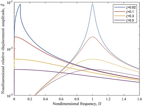
Although the frequency dependency of the excitation amplitude would not change the qualitative response of the linear system, it would affect the response of the system with a QZS spring. The main difference is that the solution is always bounded and its maximum is given by Equation (16) for a low value of damping. The amplitude of the relative displacement of the system for excitation amplitude that is changing according to a class A road profile when a vehicle travels at a speed of 110 km/hr on it is shown in Figure 3. It can be seen that the peak occurs at a lower frequency similar to what is observed for constant base excitation in Figure 2. However, the solutions are bounded and two branches of the solution always exist. The response for a low value of damping is of hardening type. It should be noted that the high amplitude of the relative displacement at a low frequency corresponds to the higher amplitude of road excitation at such frequencies due to the frequency dependency of its amplitude as described by Equations (10) and (11).

Figure 3. The frequency response curve of the relative displacement amplitude of an SDOF model for harmonic base excitations with an amplitude varying according to the road profile spectrum of a class A road at a speed of 110 km/h (${\hat{Y}}_0=$ 0.0016) for different damping ratios; solid line: QZS system, dotted lines: linear system.

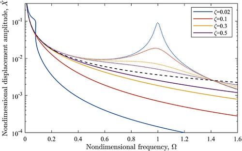
The effectiveness of the QZS spring in isolating road disturbances can be examined by obtaining the amplitude of the mass displacement. The frequency response curve of the mass displacement amplitude for the excitation amplitude equivalent to those of a vehicle travelling on a class A road at 110 km/hr is shown in Figure 4. The amplitude of excitation is plotted with a dashed line in this Figure. The QZS spring isolates the mass from the disturbances at a much lower frequency compared to its linear counterpart. For a linear spring, isolation occurs at frequencies larger than $\sqrt{2}$ while for the QZS spring with a damping ratio of $\zeta =0.02$ the nondimensional isolation frequency is about 0.08. The resonance peak has increased the isolation frequency for this damping ratio while the isolation occurs at even lower frequencies for higher values of damping ratio. Similar to a linear system, reducing the damping ratio would improve the isolation at higher frequencies at the expense of a peak in the response curve at lower frequencies. The power spectrum density of road profiles flattens at lower frequencies which would limit the amplitude of the excitation. Both linear and nonlinear systems follow the road profile for very low values of the excitation frequency as expected.

Figure 4. The frequency response curve of the mass displacement for harmonic base excitations with an amplitude varying according to the road profile spectrum of a class A road at a speed of 110 km/h for different damping ratios, (${\hat{Y}}_0=$ 0.0016); Solid line: QZS system, dotted lines: linear system, dashed line: the amplitude of the road excitation.

The response of the system to a simple harmonic excitation with a varying amplitude as that experienced by a vehicle travelling at 30 km/h on a class E is shown in Figure 5. It can be seen that for a very low damping ratio of $\zeta =0.02$, the peak is larger and the peak frequency occurs at a higher frequency. There are two fold bifurcation points in the response of the system for this damping ratio which are shown by crosses in Figure 5. There are three solutions for the amplitude at this frequency range for a very low value of damping similar to a response of the system to a constant base amplitude where two of the solutions are stable and the one that is between the two bifurcation points is unstable. However, for larger values of damping ratio, there is no visible peak in the range of interest and the isolation performance of the QZS system is superior to its linear counterpart. The damping ratio of shock absorbers is usually set in the range of 0.3–0.5. Even with a lower damping ratio of $\zeta =0.1$, there would be no peak in the response of the QZS system. The nonlinear spring would perform better in terms of isolation of road disturbances and it would not have excessive amplitude at a low-frequency resonant peak. The response of the system to transient excitation is examined in the next section by using a two degree of freedom quarter car model.

Figure 5. The frequency response curve of the mass displacement for harmonic base excitations with an amplitude varying according to the road profile spectrum of class E road at a speed of 30 km/h for different values of damping ratio, (${\hat{Y}}_0=$ 0.0157); solid line: QZS system, dotted lines: linear system, dashed line: the amplitude of the road excitation, crosses: fold bifurcations points of the nonlinear system with $\zeta =0.02$.

3. Transient response of a vehicle with a QZS spring

A two degree of freedom vehicle model is used to investigate the response of the system in the time domain. The schematic of the model is shown in Figure 6. This allows assessment of the system's performance in handling transient loads. Two types of transient loads are considered in this paper. The first is the response of the vehicle to a speed hump and the second is the response to a random road excitation for different standard road classes. The random road excitation is the same as used in the first part of this paper to obtain the frequency response curves but here the focus is on the transient response. The reaction force of the QZS spring is described by a cubic function of displacement here again and the equation of motion for the system shown in Figure 6 can be obtained, (18) $\begin{array}{rl}{m}_s{\ddot{x}}_s+c({\dot{x}}_s-{\dot{x}}_u)+k_3(x_s-x_u{)}^3& =0\end{array}$(18) (19) $\begin{array}{rl}{m}_u{\ddot{x}}_u+c({\dot{x}}_u-{\dot{x}}_s)+c_t{\dot{x}}_u+k_t{x}_u+k_3(x_u-x_s{)}^3& =k_{t}y+c_t\dot{y}\end{array}$(19) where $m_s$ is sprung mass, $x_s$ is its displacement, $m_u$ is unsprung mass, $x_u$ is its displacement, $k_t$ is the tyre stiffness and $c_t$ is the tyre damping coefficient.

Figure 6. A two degree of freedom quarter car model that is used to study the response of a vehicle with QZS springs to transient loads.

A sprung mass of $m_S=400$ kg is chosen for this study which represents approximately a quarter mass of a passenger vehicle in segment D. The unsprung mass is $m_u=80\text{kg}$ and the tyre stiffness is chosen to be $k_t=220\text{kN/m}$ [17]. Generally, passenger vehicles have a fundamental frequency in the region of 1–2 Hz [18]. Lower fundamental frequencies are used in vehicles with an emphasis on ride quality. Here, an equivalent linear spring $k_l$ is chosen in a way to have a fundamental natural frequency of ${\omega }_n=\sqrt{k_l/m_s}=1.3\text{Hz}$. The damping ratio of such a vehicle is typically about $\zeta =0.3$ [17] which is used as a reference here. The damping of the tyre is set to $c_t=839\text{Ns/m}$ which is equivalent to a damping ratio of 0.1 for the tyre-unsprung mass system [19]. The QZS spring coefficient is set to $k_3=1234\text{kN/}{\text{m}}^{\text{3}}$ which achieves the same static deformation under the vehicle weight as that of a vehicle with a linear spring. The parameter values that have been used in this study are summarised in Table 1.

Table 1. parameter values that have been used in the quarter car model.

$k_t$	220 kN/m	$c_t$	$839$ Ns/m
$k_3$	1234 kN/m^3	$c(\zeta =0.2)$	1306 Ns/m
$k_l$	26 kN/m	$c(\zeta =0.3)$	1960 Ns/m
$m_u$	80 kg	$c(\zeta =0.4)$	2613 Ns/m
$m_s$	400 kg	$c(\zeta =0.4)$	3267 Ns/m

3.1 Response to a speed hump

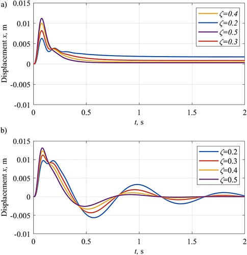
A circular arc with a length $L$ and a height $H$ is adopted as a model of a speed hump in this study [17]. The speed of the vehicle is assumed maintained while passing over the speed hump. Numerical time integration using MATLAB ode45 function is utilised to obtain the response here. The response of the vehicle travelling at 50 km/h over a hump with a height of 50 mm and a width of 600 mm is shown in Figure 7 for different damping ratios. The peak displacement is lower for the vehicle with QZS suspension than its linear counterpart for all values of damping. For a damping ratio of 0.2, the peak amplitude of the QZS suspension is about 60% of that of the linear suspension. The response is almost none oscillatory after the first peak. However, this causes the system to retain its deformed position for a longer period compared to the linear system. The retained deformation is larger for the QZS system with lower damping ratios. The lower amplitude of the response for a lower damping ratio causes a smaller secondary peak which cannot force the system back to its neutral position fast enough and the system behaves as an overdamped oscillator due to the low effective stiffness i.e. tangent to the force-deflection curve at such deformations. Since the decay is slow and without any oscillation after about 1 s, the QZS suspension should provide a more comfortable ride compared to the linear suspension which continues to oscillate for a longer period.

Figure 7. The response of the quarter vehicle model passing over a speed hump with a height of 50 mm and a width of 600 mm at 50 km/h. (a) with QZS suspension; (b) linear conventional suspension.

The vehicle acceleration needs to be kept low in order to ensure the passengers’ comfort and ride quality. The peak accelerations of the vehicle are compared in Table 2 for three different speed hump sizes. The maximum accelerations are reported for different vehicle speeds and damping ratios. The other parameters are the same as reported at the beginning of this section. A colour code with green for lower values and red for higher values is used in the table. The maximum acceleration values for all speeds, hump size and damping ratios are smaller for the vehicle with QZS suspension compared with the linear suspension. For a lower damping ratio, the difference is larger. By increasing the damping ratio, the difference between the two values is smaller but the QZS suspension maintains its benefit in terms of reduction in the maximum acceleration.

Table 2. Maximums of vehicle accelerations ${\ddot{x}}_s$ passing over different speed humps at three different speeds.

3.2. Response to random road excitation

The pseudo-random sinusoidal realisation introduced in section 2 is used to simulate road profiles here. The road profile elevation can be approximated by [16], (20) $y(s)=\sum _{i=1}^N{Y}_i\sin ({\overline{\mathrm{\Omega }}}_{i}s-{\mathrm{\Psi }}_i)$(20) where $y$ is the road elevation, $s$ is the travel distance, $Y_i$ is the amplitude which is given by Equation (11) and ${\mathrm{\Psi }}_i$ is a random uniformly distributed phase angle. ${\overline{\mathrm{\Omega }}}_1$, the lowest spatial frequency, ${\overline{\mathrm{\Omega }}}_N$, the highest spatial frequency, and $N$, the number of frequency points that are used to generate random road profile realisation, are given in the caption of Figures in this study. The response of a vehicle travelling at 90 km/h on a class B road is shown in Figure 8. For the same value of damping, the response of the vehicle with a QZS suspension is smoother and is more damped. An interesting observation is the effect of damping on the response of the QZS suspension compared to the linear one. The low damping of the linear suspension results in larger peaks as expected but for QZS suspension it causes smaller peaks due to better isolation at lower frequencies. However, a lower damping ratio for the QZS suspension results in a larger retained displacement after peaks in the road profile e.g. between 1.5 and 3 s in Figure 8. This is similar to the observation in the response to the speed hump in Figure 7.

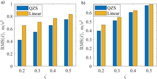
The RMS of vehicle acceleration is used here for assessing ride quality. The results for two vehicle models that are travelling at 90 km/h on a Class B road are compared in Figure 9(a). $W_b$ weighted RMS in accordance with BS 6841 [20] are compared in Figure 9(b). $W_b$ weighting may be used to assess the effect of vibration on the comfort of seated passengers in the vertical direction. The RMS acceleration is lower for the QZS suspension for any value of damping but the difference becomes less by increasing the damping ratio. There is an improvement in the response of the vehicle with QZS suspension when considering the weighted RMS but the difference between the two suspensions is less. For a damping ratio of 0.2, the reduction in RMS of acceleration is about 36% for overall RMS and about 14% for $W_b$ weighted RMS. The reduction in RMS and $W_b$ weighted RMS falls to 10% and 2% respectively for a damping ratio of 0.5.

Figure 8. The simulated road profile and the displacement response of a vehicle with different suspensions for different damping ratios. The vehicle is assumed travelling at 90 km/h on a class B road, ${\overline{\mathrm{\Omega }}}_1=0.0628$ rad/s, ${\overline{\mathrm{\Omega }}}_N=62.83$ rad/s and $N=200$. (a) road profile $y$ (thick green line) and the displacement of the vehicle $x_s$ with QZS suspension (thin lines) for two damping ratios, (b) the displacement of the vehicle $x_s;$solid lines: QZS suspension, dashed line: linear suspension.

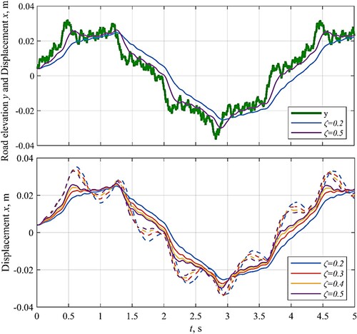
Figure 9. A comparison of RMS of vehicle acceleration for different values of damping for two vehicle models with QZS suspension and linear suspension travelling at 90 km/h on a class B road, ${\overline{\mathrm{\Omega }}}_1=0.0628$ rad/s, ${\overline{\mathrm{\Omega }}}_N=62.83$ rad/s and $N=200$. (a) unweighted RMS; (b) $W_b$ weighted RMS (BS 6841:1987).

The RMS values are also compared for a vehicle travelling at 30 km/h on a class E road in Figure 10. Here again, the QZS suspension outperforms the linear one by reducing the overall and weighted acceleration RMS values for different damping ratios. For a damping ratio of 0.2, the reduction in RMS of acceleration is about 35% due to the use of QZS suspension. For $W_b$ weighted RMS, the reduction is about 14% for a damping ratio of 0.2. . The reduction in RMS and $W_b$ weighted RMS falls to 9% and 1.5% respectively for a damping ratio of 0.5.

Figure 10. A comparison of RMS of vehicle acceleration for different values of damping for two vehicle models with QZS suspension and linear suspension travelling at 30 km/h on a class E road, ${\overline{\mathrm{\Omega }}}_1=0.0628$ rad/s, ${\overline{\mathrm{\Omega }}}_N=62.83$ rad/s and $N=200$. (a) unweighted RMS; (b) $W_b$ weighted RMS (BS 6841-1987).

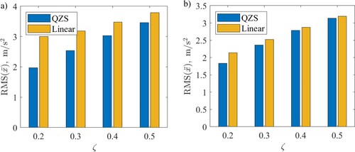
Figure 11. A comparison of weighted RMS (BS 6841:1987) of vehicle acceleration for different values of damping for two vehicle models with QZS suspension and linear suspension, rad/s, rad/s and. a) travelling at 90 km/h on a class B road; b) travelling at 30 km/h on a class E road.

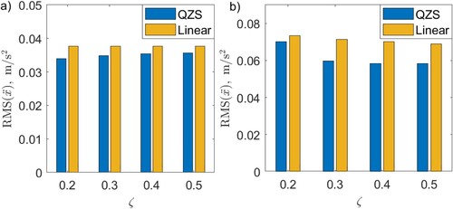
BS 6841 provides $W_f$ weighting to assess the effect of vibration on motion sickness for which low frequencies of 0.1 Hz to 0.5 Hz are assessed. $W_f$ weighted RMSs for the above two cases are shown in Figure 1. The vehicle with a QZS suspension outperforms the linear suspension for all damping ratios and also for both travelling speeds. Unlike the previous cases the reduction in $W_f$ weighted RMS increases by increasing the damping ratio. The QZS suspension improves the isolation at very low frequencies which resulted in a lower level of $W_f$ weighted RMS of the vehicle acceleration.

4. Discussions

One of the main issues with the implementation of a QZS spring in a vehicle suspension is the possibility of an unbounded response to harmonic base excitations. However, such responses only occur for a low damping ratio with a high amplitude of base excitations which are unlikely for vehicles. For a base-excited SDOF system, the damping ratio $\zeta$ should be smaller than $\left(\sqrt{3\gamma }\hat{Y}\right)/4$ in order to have an unbounded response. Assuming a fundamental frequency of 1.3 Hz for the equivalent car with a linear suspension and a nondimensional nonlinear stiffness of unity ($\gamma =1$) as discussed in Section 2, the solution would be unbounded for a damping ratio of $\zeta \le 0.063Y$ which is unlikely in practice.

More importantly, it is shown that since road disturbance amplitude is inversely proportional to their spatial frequency, the response of the system with a QZS spring would be always bounded. The peak in the frequency response curve of the system with a QZS spring vanishes for damping ratios larger than 0.1 as shown in Figures 3 and 4. The high damping ratio in vehicle suspension controls the amplitude of the peak about the fundamental frequency of the suspension but it adversely affects the suspension performance in isolating road disturbances at higher frequencies. Since there is no peak in the response of the QZS system for damping ratios higher than 0.1, it is reasonable to use a QZS suspension system with a lower damping ratio and benefit from better isolation at high frequencies.

A vehicle fitted with a QZS suspension would experience reduced disturbances when passing over a speed hump compared to a vehicle with linear suspension. Increasing the damping ratio would result in a higher amplitude for the response. However, an issue is a residual displacement due to the disturbance. The lower amplitude of the response at low damping ratios, although desirable, causes the system to operate in the vicinity of the loaded position where the effective stiffness is low. Such a low effective stiffness changes the behaviour of the system to an overdamped oscillator with a low rate of change which results in a residual displacement in the vehicle response. This may undermine using lower values of damping for the QZS suspension although it can provide better isolation from road disturbances. This may necessitate the use of the QZS suspension alongside a self-levelling system.

A linear damper model is used in this study while the vehicle shock absorbers are designed to behave nonlinearly. A different design for the shock absorber and/or increasing the minimum stiffness to a non-zero value can resolve this issue which is out of the scope of this paper.

The response of the vehicle to random road disturbances follows a similar trend. The response of a vehicle with QZS suspension is smoother and high-frequency disturbances are better isolated compared to the linear isolator. The values for both types of weighted acceleration RMS that are used in this study are lower for the vehicle with the QZS suspension which confirms the improvement in the ride quality of such vehicles.

5. Conclusions

An SDOF model and a quarter car model are used in this study to investigate the possibility of using QZS springs in vehicle suspension. It is known that the frequency response curve of a base excited SDOF system with a QZS spring can be unbounded. This potentially can lead to vehicle instabilities that undermine the usability of QZS springs for vehicle suspensions. However, it is shown here that the inverse dependency of the road profile amplitude to spatial frequency would result in a bounded response for a system with a QZS spring.

For low values of damping, there could be a hardening type behaviour in the response curve of the QZS system with a peak at a lower frequency compared to the linear system. But this is unlikely in practice due to the high level of damping employed in a vehicle suspension. The peak disappears in the frequency response curve of the QZS system for damping ratios as low as 0.1. Thus, it is suggested to use a lower value of damping for vehicle suspension using QZS springs which can improve isolation at higher frequencies. Even, with the same damping ratio as linear suspensions, the isolation from road disturbances occurs at much lower frequencies and there is a noticeable benefit in employing QZS springs.

The response of the suspension with QZS springs to transient disturbances is examined using a two degree of freedom quarter car model by simulating the vehicle response when passing over a speed hump and to random road excitations. The maximum and weighted RMS of acceleration are used to evaluate the performance of the suspension. In both cases, the QZS suspension provided better isolation of road disturbances. However, there is a residual displacement in the response of the vehicle with low damping ratios due to the lower effective stiffness of the QZS suspension. More complex models may be used to investigate such behaviour further. A QZS suspension may be used in parallel to a self-levelling system to overcome the problem of retained displacement.

Disclosure statement

No potential conflict of interest was reported by the author.

References

- Alabuzhev P. Vibration protection and measuring systems with quasi-zero stiffness. Washington (DC): Hemisphere; 1989.
- Ibrahim RA. Recent advances in nonlinear passive vibration isolators. J Sound Vib. 2008;314(3-5):371–452.
- Liu C, Jing X, Daley S, et al. Recent advances in micro-vibration isolation. Mech Syst Signal Process. 2015;56-57:55–80.
- Carrella A, Brennan MJ, Waters TP, et al. Force and displacement transmissibility of a nonlinear isolator with high-static-low-dynamic-stiffness. Int J Mech Sci. 2012;55(1):22–29.
- Kovacic I, Brennan MJ, Waters TP. A study of a nonlinear vibration isolator with a quasi-zero stiffness characteristic. J Sound Vib. 2008;315(3):700–711.
- Anubi OM, Patel DR, Crane Iii CD. A new variable stiffness suspension system: passive case. Mech Sci. 2013;4(1):139–151.
- Saini M. Modelling and simulation of vehicle suspension system with variable stiffness using quasi-zero stiffness mechanism. SAE Int J Veh Dyn Stab NVH. 2020;4(1):37–47.
- Li SH, Yang SP, Guo WW. Investigation on chaotic motion in hysteretic non-linear suspension system with multi-frequency excitations. Mech Res Commun. 2004;31(2):229–236.
- Litak G, Borowiec M, Friswell MI, et al. Chaotic vibration of a quarter-car model excited by the road surface profile. Commun Nonlinear Sci. 2008;13(7):1373–1383.
- Litak G, Borowiec M, Friswell MI, et al. Chaotic response of a quarter car model forced by a road profile with a stochastic component. Chaos Soliton Fract. 2009;39(5):2448–2456.
- Zhou SH, Song GQ, Sun MN, et al. Nonlinear dynamic analysis of a quarter vehicle system with external periodic excitation. Int J Nonlin Mech. 2016 Sep;84:82–93.
- Zeng YC, Ding H, Du RH, et al. A suspension system with quasi-zero stiffness characteristics and inerter nonlinear energy sink. J Vib Control. 2020;28(1-2):143–158.
- International Organization for Standardization (ISO). (2016). Mechanical vibration – Road surface profiles – Reporting of measured data. Switzerland: ISO. Standard No. ISO8608:2016.
- Carrella A, Brennan MJ, Waters TP. Static analysis of a passive vibration isolator with quasi-zero-stiffness characteristic. J Sound Vib. 2007;301(3):678–689.
- Milovanovic Z, Kovacic I, Brennan MJ. On the displacement transmissibility of a base excited viscously damped nonlinear vibration isolator. J Vib Acoust. 2009;131(5):054502. 1-7.
- Rill G. Road vehicle dynamics: fundamentals and modeling. Boca Raton (FL): CRC Press; 2011.
- Garcia-Pozuelo D, Gauchia A, Olmeda E, et al. Bump modeling and vehicle vertical dynamics prediction. Adv Mech Eng. 2014 Jan;6:736576.
- Blundell M, Harty D. The multibody systems approach to vehicle dynamics. Amsterdam: Elsevier; 2014.
- Maher D, Young P. An insight into linear quarter car model accuracy. Veh Syst Dyn. 2011;49(3):463–480.
- British Standards Document BS 6841. (1987). Guide to measurement and evaluation of human exposure to whole-body mechanical vibration and repeated shock. UK: BSI; Standard No. BS 6841:1987.