Wheel wear reduction of a mechatronic two-axle vehicle controlled with feedforward wheelset steering approaches

Abstract

The mechatronic vehicle developed within the Shift2Rail projects Run2Rail, Pivot, NEXTGEAR, and Pivot2 is evaluated with respect to wheel wear. The KTH wear model is used to determine the coefficients of Archard’s wear map to reproduce measured worn wheel profiles of the present vehicle running on Metro Madrid line 10. The same wear model is then used to evaluate the performance of the mechatronic vehicle controlled with two variants of a feedforward controller. The first one uses on-board measurements, while the second one is optimised using firefly optimisation algorithms assuming knowledge of the travelled track. The control strategy based on on-board measurements shows improvements above 60% in terms of lost wheel volume due to wear, compared to the standard bogie vehicle. The optimised controller reaches improvements above 70%. Good coherence is found between improvements predicted with the wear number and the ones achieved in terms of lost wheel volume.

KEYWORDS:

• Two-axle mechatronic vehicle
• feedforward active steering control
• firefly algorithms
• KTH wear model
• experimental data fitting

1. Introduction

Wheel wear is among the key aspects that affect railway maintenance. It can cause passenger discomfort and running instability. Therefore, the wear development is of great importance. Wheel wear is influenced by various factors, among which, traction, braking, and wheelset guidance show the largest influence. Concerning the last point, active wheelset steering can significantly reduce wheel wear [1], overcoming the well-known trade-off between running stability and steering capability of passive suspensions. Several studies on active wheelset steering have shown great potential in reducing the wheel-rail contact forces [2]. Nevertheless, only few field studies are reported in the literature [3,4] due to, among other reasons, concerns about safety issues in case of actuator failure [2,5].

With exception of Fu et al. in [1] who evaluated wheel wear with different known steering strategies, the steering control design [4,6] and steering control performance are evaluated with help of the wear number $T\gamma$, which is very easy to calculate with standard outputs from multibody simulations. $T\gamma$ is an engineering quantity expressing the amount of energy dissipated in the wheel-rail contact per travelled distance [7] and can effectively be used for comparisons (see Section 6). However, it can suffer in predicting the wheel wear evolution due to lack of information regarding the local stress conditions in the contact patch between wheel and rail [8,9]. Other methods can be implemented to handle this influence better, such as the KTH wear model based on Archard’s wear map [10,11] used in this work.

The innovative two-axle vehicle developed in the Shift2Rail projects Run2Rail, Pivot, NEXTGEAR, and Pivot2, has shown great potential in terms of $T\gamma$ performance [6]. Nevertheless, the performance in terms of wheel wear evolution is unknown and is therefore the focus of this study. The two-axle vehicle is meant to be a substitute for the Metro Madrid line 10 vehicle S8000. To showcase the benefit of the new mechatronic vehicle, wheel wear is compared with the one of the S8000 after tuning of Archard’s wear map coefficients to reproduce measured worn wheel profiles.

The innovative vehicle is equipped with active wheelset steering controlled by a feedforward approach. This approach avoids the use of quantities that are difficult to measure, such as the lateral wheelset displacement with respect to the track centreline and the wheelset attack angle. These quantities may be estimated with modern Kalman filters [12–14]. Nevertheless, the effectiveness of these methods does not guarantee stability of the feedback controllers that may suffer from non-linearities and unmodelled behaviours.

Two feedforward steering control strategies are tested here. The first one has previously been developed by the authors and it has been shown to be robust against conicity, vehicle speed, and track curvature variation [6]. The second feedforward steering strategy relies on the hypothesis that the infrastructure and the running vehicle have a close communication, and that the steering control can be commanded based on the vehicle location on the track and its speed. The force commands and their timing with respect to the track are optimised with firefly algorithms (FAs) [15,16].

The hypothesis to be tested is that the innovative two-axle vehicle can reduce the lost wheel volume compared to the present vehicles and that a wheelset steering controller based on the vehicle location on the track can further enhance the benefit.

2. Methodology and wear calculation

The wheel wear evolution is determined with the KTH wear model based on Archard’s wear map [10,11]. Firstly, the load collective is established based on nominal track data form Metro Madrid line 10. Subsequently, the Archard’s wear map coefficients are tuned to fit measured worn wheels with a simulated S8000 bogie vehicle (presently running on line 10). The wheel wear evolution of the innovative mechatronic vehicle is then evaluated using the Archard wear coefficients obtained during the tuning phase. The mechatronic vehicle is controlled with two steering control techniques as mentioned in the introduction. The methods will be explained in Section 4.

The wear calculation methodology used has been shown to be effective in reproducing experimental results [10,17–20] and to have a good performance in comparison with other methods [9]. The KTH method has also been applied to maintenance optimisation and prediction for both wheels [21] and rails [22].

The simulated worn wheel profiles are obtained through the following steps.

1. Contact patch wear

Hertz contact is applied to calculate the normal pressure, while FASTSIM is used to calculate the tangential stresses. For each contact patch the normal wear is calculated as (1) $\mathrm{\Delta }z\left(x,y\right)=K_n\frac{p\left(x,y\right)s\left(x,y\right)}{H},$(1) where $\mathrm{\Delta }z\left(x,y\right)$ is the removed material in the local contact patch coordinates $x$ and $y$ and it is measured in meters, $K_n$ is Archard’s wear coefficient, $p\left(x,y\right)$ is the normal pressure, $s\left(x,y\right)$ is the slip distance, and $H$ is the hardness of the wheel [10]. The normal contact patch wear has a discretization equal to the discretization used in the FASTSIM algorithm. The hardness of the material for the present study is set to 2.8e3 MPa [7]. Hertz normal pressure and FASTSIM tangential stresses models have been chosen over other normal and tangential contact problem models due to their well-established and fast computation.

1. Transformation of the patch wear to the wheel coordinate system

The method assumes uniform wear over the entire wheel circle. Thus, the three-dimensional normal wear (Equation (1)) is represented in a two-dimensional space, (2) $\mathrm{\Delta }Z\left(y\right)=\sum _{x=-a}^a\mathrm{\Delta }z\left(x,y\right),$(2) where $\mathrm{\Delta }Z\left(y\right)$ is the normal wear as function of the local contact patch coordinate $y$, and $a$ is the longitudinal contact patch dimension. The obtained normal wear is re-discretized in the wheel profile lateral coordinate $y_p$ discretization and centred in the contact point location from $-b$ to $b$, where $b$ is the lateral contact patch dimension.

1. Calculation of normal wheel wear per load case

Being the wear assumed uniform over the wheel diameter, $\mathrm{\Delta }Z\left(y_p\right)$ is evaluated every wheel turn, giving a total $N=L^{sim}/\left(2\pi r_0\right)$ number of points to be evaluated for every simulated length $L^{sim}$ with a wheel of nominal radius $r_0$. The normal wheel wear per load case, (3) ${\hat{W}}_j\left(y_p\right)=\sum _{k=1}^5\sum _{i=1}^N\mathrm{\Delta }{Z}_{i,k}\left(y_p\right),$(3) is simply evaluated as the sum of each individual contribution over the simulated interval. The procedure is repeated for each contact patch (with a maximum of five contact patches calculated in SIMPACK).

1. Calculation of normal non-dimensional wheel wear

The normal wheel wear is calculated based on the track information through the representative share $r_j$ of each simulated load case (Table 1). Each load case is normalised by its respective simulated length $L_j^{sim}$, producing the normal non-dimensional wheel wear, (4) $\hat{W}\left(y_p\right)=\sum _{j=1}^{N_L}\frac{1}{2}\left({\hat{W}}_j^L\left(y_p\right)+{\hat{W}}_j^R\left(y_p\right)\right)\frac{r_j}{L_j^{sim}},$(4) where ${\hat{W}}_j^L$ and ${\hat{W}}_j^R$ represent the normal wheel wear per load case developed on the left respectively right wheel, and $N_L$ is the number of load cases. The procedure is repeated for each wheelset, considering an equal amount of right-hand and left-hand curves.

1. Scaling strategy

Table 1. Load collective for Metro Madrid line 10.

	NLA [m/s^2]	Curve Radius $\tilde{R}$ [m]	Cant $\tilde{h}$ [mm]	Speed $v$ [km/h]	Transition curve length ${\tilde{L}}_{tr}$ [m]	Circular curve length ${\tilde{L}}_{cr}$ [m]	Simulated distance $L^{sim}$ [m]	Cumulative length $L_{tr}+L_{cr}$ [m]	Representative share $r$ [%]
S-Curve	§	§	§	30	§	§	192	132	0.3%
	0.61	272	87	64	40	114	254	2314	5.9%
200 ≤ R ≤ 300	0.28	267	96	56	66	107	299	2273	5.8%
	−0.07	258	110	47	66	136	328	1201	3.1%
	0.70	350	53	69	55	287	457	2376	6.1%
300 < R ≤ 400	0.41	359	108	72	60	181	361	2868	7.3%
	0.13	348	131	67	67	193	387	1801	4.6%
	0.49	455	75	76	66	198	390	1152	2.9%
400 < R ≤ 600	0.21	489	93	72	87	105	339	1953	5.0%
	−0.19	502	76	45	34	76	204	788	2.0%
600 < R ≤ 800	0.46	744	25	78	63	92	278	873	2.2%
	0.06	722	42	56	42	71	215	1320	3.4%
800 < R ≤ 1200	0.31	977	10	69	33	108	234	785	2.0%
	−0.05	1067	40	54	13	47	133	220	0.6%
1200 < R ≤ 2000	0.12	1753	10	65	67	135	329	804	2.0%
Tangent	§	§	§	60	§	§	1000	9209	23.4%
	§	§	§	70 → 1	§	§	Variable	9209	23.4%

The normal non-dimensional wheel wear is scaled to an allowed amplitude in order to obtain the dimensional form of the normal wear. The scale-up, (5) $S=\frac{0.1\cdot {10}^{-3}}{{\hat{W}}_{max}},$(5) is obtained by dividing the maximum allowed wear of 0.1 mm by the maximum of the normal wear ${\hat{W}}_{max}$ among all the wheels. The scale-up $S$ is expressed in meters and represents the distance travelled by the vehicle. To avoid excessive travelled distances, the scale-up is limited to 2000 km. The dimensional normal wear is then simply calculated for each wheel as ${\hat{W}}^N=S\cdot \hat{W}$.

1. Definition of worn wheel profiles

The normal wear is applied to the wheel profiles following simple trigonometric functions to calculate the new lateral and vertical profile coordinates using the wheel angle $\gamma$,¹ (6) $\{\begin{array}{c}{y}_p^{new}=y_p-{\hat{W}}^N\left(y_p\right)\cdot \sin \left(\gamma \left(y_p\right)\right)\\ z_p^{new}=z_p-{\hat{W}}^N\left(y_p\right)\cdot \cos \left(\gamma \left(y_p\right)\right)\end{array},$(6) where the wheel angle, (7) $\gamma =\mathrm{arctg}\left(\frac{d{z}_p}{d{y}_p}\right),$(7) is the geometric angle of the wheel in the lateral-vertical wheel profile coordinate system calculated for the previous wear step worn profile.

Once the new coordinates are defined, the vertical wheel profile coordinate needs to be re-discretized on the original profile lateral coordinates. This avoids numerical problems in the simulations, keeping the profile lateral coordinates monotonically increasing. The profiles are finally smoothened with a moving mean of 5 points every 10 wear steps.

1. Wheel position exchange for runs in the reverse direction

Depending on the operational scenario of the simulated vehicle, the wheels need to change positions between the simulation sets. For the analysed line, the vehicle runs in one direction and subsequently the other direction. Going from end station A to B and back, the part of the vehicle that is leading is exchanged between the ‘front’ and the ‘rear’ part of the vehicle itself. This means that the leading wheelset left wheel will become the trailing wheelset right wheel and vice versa.

The vehicle simulations for the defined load collective and the steps described above constitute a wear step. This is repeated until the simulated travelled distance (sum of the scale-up $S$ in every wear step) meets or exceeds the required one. The latter is set to 150.000 km equal to the wheel reprofiling interval of the present vehicles.

3. Track analysis and assumptions

3.1. Track analysis

In the evaluation of uniform wheel wear, the representation of the track and the wheel rail contact conditions have paramount importance. Depending on the track, the wheel wear obtained with the same vehicle can be significantly different.

To properly represent the running conditions in a simulation environment, the track analysis can be divided into three main aspects, i.e. statistical analysis of the track on which the vehicle is running (defining the load collective), wheel-rail contact conditions, and the assumptions required for simulation purposes or by lack of real-world data.

3.1.1. Statistical analysis (load collective definition)

Following the KTH method for evaluating uniform wheel wear, the track on which the vehicle is running can be split into several load cases, constituting the load collective. The load cases are needed to reduce the computational burden required to perform the wear evaluation. At the same time, dividing the track into several load cases provides control over the wheel wear evolution during the tuning phase of Archard’s wear coefficients, giving the possibility of analysing the results over a reduced number of cases. Nevertheless, to have representative meaning, the load cases need to be chosen based on a statistical evaluation of the travelled track.

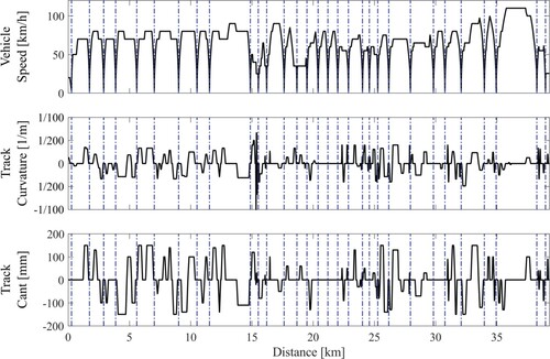
In Figure 1, the nominal vehicle speed, track curvature, and track cant for line 10 of Metro Madrid are shown. As expectable from a metro line, the amount of small radius curves and vehicle speed variation is significant.

Figure 1. Nominal line 10 data: (Top) vehicle speed, (Centre) track curvature, and (Bottom) track cant. The solid line shows the nominal data while the dashed lines represent stations.

The statistical analysis of the track is performed starting with the definition of significant curve sections. With reference to Figure 2(A), it can be noticed that the track curve radii are greater than 200 m (−1/200 ≤ 1/R ≤ 1/200), with exception of the s-curve shown in Figure 2(B). This s-curve comprises a 100 m curve followed by two 150 m curves. It represents an outlier that is therefore removed from the statistical analysis and kept as an individual load case. Tangent track sections are also excluded from the statistical analysis of the curved sections and are considered as a separate load case.

Figure 2. Line 10 statistical analysis. (A) line 10 nominal track curvature, (B) detail of the s-curve curvature, (C) occurrence of curves for curve radii greater than 200 m, and (D) K-means clustering for each curve family of (C). In (D), for each curve family, each curve is shown with a marker corresponding to the cluster it belongs to. Each cluster centroid is shown with a dashed line.

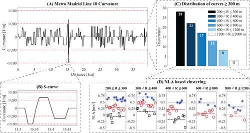
In Figure 2(C), the occurrence of specific curve radii is shown divided into curve radius families. Here, the curve families’ range is selected to produce a reasonable representation of the track. It can be noticed that the number of very small curve radius track sections (R ≤ 400) is higher than the number of medium, and medium-high curve radius sections. Additionally, it should be noted that the track sections with curve radius between 1200 m and 2000 m are only three. Despite the low count, these curves represent 2% of the track in terms of distance and cannot be neglected (see Table 1).

Once the curve families are defined, the information about vehicle speed and track cant can be considered. For each curve in each curve family, the non-compensated lateral acceleration (NLA) can be calculated, (8) $NLA=\frac{v^2}{R}-g\frac{h}{2b_0},$(8) where $v$ is the vehicle speed in m/s, $R$ is the curve radius in m, $g$ is the gravitational acceleration, $h$ is the track cant in m, and $b_0$ is the nominal radius distance from the centre of the track in m. Based on the NLA, within each curve family, a second selection is made to handle the variations in NLA that exist and would disappear if only one average were taken in each curve family. The K-means clustering method [23] is used to automatically determine these last subcategories. The clusters’ centroids determine the required NLAs for the specific curve family, being the cluster centroid the value that has the minimum distance between itself and each other point in its cluster. In Figure 2(D), the K-means clustering for each curve family is shown. The curve family 1200 < R ≤ 2000 is excluded from the clustering as there are only three curves in the family.

Each cluster defines a load case. For each load case, the average curve radius $\tilde{R}$, average track cant $\tilde{h}$, average transition curve length ${\tilde{L}}_{tr}$, cumulative circular curve length $L_{cr}$, and cumulative transition curve length $L_{tr}$ are collected. Each load case is built assigning a circular curve section NLA equal to the corresponding cluster centroid, and a curve radius and a track cant equal to the average ones for that cluster, i.e. $\tilde{R}$ and $\tilde{h}$. The desired vehicle speed is then back calculated starting from Equation (7), (9) $v=\sqrt{\frac{1}{\tilde{R}}\left(NLA+g\frac{\tilde{h}}{2b_0}\right)}.$(9)

An exception is represented by the curve family 1200 < R ≤ 2000, where the required NLA is calculated as the average between the three curves. The transition curve length is assigned to be the average per cluster, while, to maintain the same transition curve to circular curve ratio approximating the one in line 10, the circular curve length is calculated as (10) ${\tilde{L}}_{cr}=2{\tilde{L}}_{tr}\frac{L_{cr}}{L_{tr}}.$(10)

Finally, the representative share of each load case over the total length of line 10 is calculated as the ratio between the sum of the cumulative lengths and the total length $L_{tot}$ of line 10, $r=\left(L_{tr}+L_{cr}\right)/L_{tot}$.

In Table 1, the 17 designed load cases are presented. These are composed of 14 curve load cases defined by the statistical analysis of the curve sections distribution (13 cases from the NLA clustering (Figure 2(D)) plus one for the 1200 < R ≤ 2000 curve family), one s-curve, and two tangent track sections. The tangent track section has been split into two halves, one with the vehicle travelling at a constant speed and one with braking. This assumption is further discussed in Subsection 3.2. To properly simulate the 14 curve load cases, a 30 m tangent track is applied before and after the negotiated curve giving a simulated distance of $L_{sim}=2{\tilde{L}}_{tr}+{\tilde{L}}_{cr}+60$. The same tangent track sections have been applied to the simulated s-curve.

3.1.2. Wheel-rail contact conditions

The second fundamental aspect to be considered is the wheel and rail interaction. Different wheel and rail profiles will cause different wheel wear evolution given the same load cases. The nominal wheel profile used is the standard S1002 profile while the rail profile is the 54E1 rail with an inclination of 1:20. The nominal track gauge is 1.445 m. The defined wheel and rail combination results in the contact conditions shown in Figure 3(Top-left) and the conicity profile shown in Figure 3(Right).

Figure 3. Wheel-rail contact conditions: (Top-left) contact overview showing the nominal wheel and rail profiles and the possible contact points, (Bottom-left) wayside lubrication showing the variation of the friction coefficient in red against the nominal rail profile in black, and (Right) equivalent conicity profile for the nominal wheel and rail condition calculated in SIMPACK. In this last, the dash-dotted line shows the conicity at 3 mm amplitude.

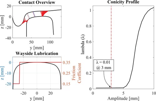
Metro Madrid applies lubrication to the outer rail for curve radii smaller than 1000 m with the purpose to reduce the adhesion between rail and wheel flange and thereby reduce wear on rails and wheels. Wayside lubrication is simulated by a change in the friction coefficient depending on the lateral rail coordinate. This is easy to model thanks to the contact model in SIMPACK. Being the friction unknown in the real operation, a friction coefficient is assigned to be 0.35 in the non-lubricated points and 0.15 in the lubricated ones.² In Figure 3(Bottom-left) the influence of wayside lubrication on the friction coefficient is shown. The transition between low and high friction coefficients is approximated by a steep linear transient. No modifications of the friction coefficients are applied since line 10 can be considered a closed system being completely underground.

3.2. Simulation assumptions

Several assumptions are made to model the vehicle and vehicle-track interaction and to overcome the lack of experimental and real-world data. These assumptions are summarised hereafter.

1. Trailer vehicle

The mechatronic vehicle is under development and what is available is a simulated virtual vehicle for which the traction equipment has yet to be designed in detail. Therefore, the focus is kept on the trailer car, and thus no traction is considered.

1. Rail profiles

As described in Subsection 3.1.2, rail profiles are among the key factors that influence the evolution of the wheel wear. Worn rail profiles are not available and new rail profiles are used independently from the load case. This assumption may lead to a different shape of the wheel wear especially in the region where new wheel and rail profiles do not have any possible contact points (Figure 3(Top-left)).

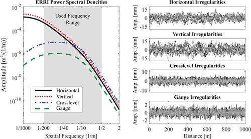
1. Track irregularities

The track irregularities of Metro Madrid line 10 are not available either. Thus, ERRI power spectral densities (PSD) [24] are used to generate the track irregularities. Specifically, ERRI_High track irregularities are used to represent horizontal, vertical, and cross-level irregularities. According to [25], gauge irregularities can be generated from a spectrum equivalent to the one for ERRI cross-level. In Figure 4(Left), the four PSD used are shown together with the considered spatial frequency range used in the simulations. At the beginning of each simulation, the track irregularity profiles are randomised to increase the variability of the system. In Figure 4(Right), a sample of 10 randomised track irregularity profiles is shown.

1. Track gauge widening

Figure 4. Track irregularities: (Left) ERRI power spectral density showing the frequency region used in the simulations, (Right) randomly generated track irregularities profiles

Track gauge widening is related to tight curves. To simulate this effect, the nominal gauge is increased by 2.5 mm for curves with a radius smaller than 300 m, while it is increased by 1.25 mm for curves with curve radius between 300 and 600 m.

1. Vehicle speed

Being the focus on the trailer vehicle, the speed is considered constant for all the load cases with exception to the breaking load case. A constant speed is assigned to the carbody simulating it being pulled or pushed by a motorised car. High slip in the contact patch may be achieved during traction or braking influencing the wear. Thus, a braking case is introduced. For the sake of simplicity, braking is assumed to take place in half of the available tangent track length (Table 1). Here the vehicle speed is reduced from approximately 70 to 1 km/h trough a constant braking torque applied to the wheelsets.

To simulate the speed’s variability intrinsic in a metro line system, the vehicle speed at the beginning of each simulation is randomised within a 5% interval of the nominal speed given in Table 1. The same applies to the initial speed of the braking section.

1. Archard’s wear maps

Due to the presence of way side lubrication, two Archard maps are used both in the tuning phase and in the evaluation phase. This assumption allows better adaptability during the tuning phase, keeping the physical meaning of Archard’s wear model.

4. Vehicles and control strategies

Both the standard bogie vehicle and the mechatronic vehicle are modelled in SIMPACK and are described hereafter. For the mechatronic vehicle, two control strategies for the wheelset steering are introduced.

4.1. Standard bogie vehicle

The vehicle S8000, presently running on Metro Madrid line 10, represents the benchmark condition that the mechatronic vehicle is compared to. Each car of the S8000 vehicle consists of a carbody with mass of approximately 30 tons, two bogies with mass of 3 tons, and four wheelsets with mass of 1.8 tons. The vehicle is composed by two motorised end cars, and an intermediate trailer car, giving a tare weight per meter of approximately 1900kg/m. The vehicle has a maximum allowable speed of 120 km/h and a nominal wheel radius of 0.43 m. These last two properties are shared with the mechatronic vehicle. More information can be found in [26].

4.2. Mechatronic vehicle

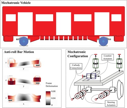
The mechatronic vehicle has been developed to be a substitute of the S8000 standard bogie vehicle presented in Subsection 4.1. The objective is to reduce the tare weight and maintenance costs. To do so, the mechatronic vehicle has two single axle running gear, i.e. only two axles per vehicle. For further weight saving, a U-shaped connection frame in carbon fibre reinforced polymer is designed. This frame also acts as anti-roll bar. The expected saving in terms of tare weight per vehicle meter is about 400 kg/m. Thanks to the weight reduction, energy savings of about 5% to 8% per run on line 10 are expected [27]. However, this type of two-axle vehicle may suffer from poor steering capability, due to the long distance between the wheelsets, and poor passenger comfort due to only one suspension step. Thus, active suspensions are introduced both to improve steering and comfort of the vehicle. A detailed description of the vehicle configuration is given in [28], while in [29] and [30] the design of the steering actuators and the U-shaped connection frame are described respectively. In [31,32] the comfort problem is addressed, and control strategies are proposed showing the possibility of maintaining comfort levels within the limits given in EN12299 [33].

In Figure 5 an overview of the mechatronic vehicle is given. The vehicle is simulated in SIMPACK where flexible modes of the carbody and the U-frame are imported from Finite Element models in Abaqus. The five hydraulic actuators (three for comfort and two for steering on each running gear) are simulated in Simulink-Simscape. The hydraulic comfort actuator [32] is modelled based on actuators used in field applications [34,35]. The steering actuator is a hydraulic actuator developed in the Shift2Rail project NEXTGEAR [29] and it is designed to provide both hunting stability and steering actuation forces. Hunting stability is achieved by having disc springs inside the actuator providing wheelset yaw stiffness. The configuration results in a two-zone non-linear stiffness, where a higher stiffness of 8 MN/m is provided in the central zone (wheelset displacement within 1.5 mm) and a lower 4 MN/m stiffness is obtained in the external zone (wheelset displacement larger than 1.5 mm). The central stiffness zone provides hunting stability, while the lower stiffness in the external zone reduces the force needed to steer the wheelset to correct position during curving. A detailed description of the trade-off between curving capability and hunting instability of the non-linear stiffness is given in [36]. Two steering actuators acting on the same axle are cross-coupled. The pressure inside each of the cross coupled chambers is controlled via a pressure-controlled valve, that allows to vary the pressure proportionally to a command current. The combined effect of the inbuilt two-zone non-linear stiffness and the pressure-controlled valves make the steering actuator act both as a suspension element and an actuator. The model developed in Simscape has been tuned to fit experimental results [29].

Figure 5. Mechatronic vehicle configuration: (Top) mechatronic vehicle overview, (Bottom-left) anti-roll bar motion of the U-shaped frame showing the frame deformation, and (Bottom-right) arrangement of the actuators connecting the single axle running gear to the carbody.

Due to the high percentage of very small curve radius track sections, the wheel wear evolution is mainly influenced by the steering capability of the vehicle. Therefore, hereafter, two steering control approaches are presented. The first one was developed previously by the authors in [6] and will be shortly summarised, while the second one is introduced here.

4.2.1. Original feedforward controller

The steering control strategy developed in [6] is a feedforward approach that is robust against conicity, velocity and curvature variation. The controller takes as inputs the NLA and the curvature of the track and produces a steering force, (11) $F=k_{1}NLA\left(\frac{1}{R}\right)+k_2\left(\frac{1}{R}\right)+k_{3}NLA+k_4,$(11) where the coefficients $k_j$ are different for the leading and trailing wheelsets producing a different command steering force for the two wheelsets. The controller has been designed through a comparative study of several feedback steering command signals, amongst which were radial steering and perfect steering. Starting from the results obtained with the feedback controllers, a combination of the wheelsets’ wear number $T\gamma$ and steering control force have been used to determine a steering force surface as a function of the NLA and curvature. The coefficients of Equation (10) let the feedforward control force approximate the steering force surface. The control force is then limited to 40 kN to avoid safety issues in case of an actuator malfunctioning while it is set to 0 kN for curve radii greater than 2000 m.

The feedforward controller does not rely on quantities that are difficult to measure (wheelset lateral displacement or attack angle). Nevertheless, the controller requires the knowledge of the NLA and the curvature. The NLA can be estimated by an accelerometer in the running gear while the curvature can be derived by a yaw rate gyroscope in the carbody centre ${\dot{\phi }}_c$ combined with a tachometer to obtain the vehicle speed $v$, (12) $\frac{1}{R}=\frac{{\dot{\phi }}_c}{v}.$(12)

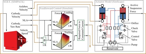
In Figure 6, a schematic overview of the control loop is shown. Here, the steering hydraulic actuators scheme is shown too. The SIMPACK module (Left of Figure 6) provides the NLA, the carbody yaw rate, and the vehicle speed needed to calculate the steering forces. Additionally, it provides the axlebox and carbody velocities at the actuators’ connection location for each actuator. These are needed to properly calculate the response of each actuator to the vehicle stimuli. In addition to the above-described feedforward control approach, the control module (Centre of Figure 6) translates the required steering command forces to current signals to be provided to the pressure-controlled valves. The actuator module (Right of Figure 6) accepts the vehicle stimuli provided by SIMPACK and the current command produced by the feedforward controller and generates the active suspension forces to be fed back to SIMPACK. The active suspension forces are a combination of the chamber force and the non-linear spring stiffness. In absence of a command signal, the actuator models produce the spring force to ensure vehicle hunting stability.

Figure 6. Control loop showing the key aspects from the multi body simulation of the vehicle in SIMPACK, through the control logic in Simulink, and to the actuator model in Simscape. Note that in the Figure (on the right) the vehicle stimuli (axlebox and carbody velocity) are provided to the left actuator while the suspension force is produced by the right actuator. This only make the figure easier to read, in the simulations all actuators receive the vehicle stimuli and produce the suspension forces.

4.2.2. On-purpose optimised controller

To be applicable to any condition, the feedforward controller requires to have the NLA, the carbody yaw rate and the vehicle speed to be measured onboard. This makes the controller suffer from filtering effects (to avoid track irregularity influence) and intrinsic delays (particularly for the leading wheelset but also with a certain delay in the trailing one). The combination of the two produces delays in the activation of the steering command forces negatively influencing the performance in the transition curve sections. Such effect may influence the wheel wear evolution due to an incorrect position of the wheelset in transition curve sections.

To overcome this issue, optimised steering control signals can be studied, which means to substitute the feedforward control module of Figure 6 with dedicated command signals to be provided directly to the actuators control valves. Thus, the relation between the vehicle behaviour and the steering command is removed. For each of the 14 curve load cases plus the s-curve, a deterministic command signal will be derived. This procedure removes the generality of a robust generally working controller in favour of an on-purpose single-objective controller. This controller has the objective of investigating possible improvements of a line dedicated steering controller that does not rely on on-board vehicle measurements but on vehicle-infrastructure communication.

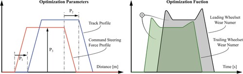
During preliminary investigation, it was observed that an anticipation (or preview) of the force command with respect to the track transition curve initiation could decrease the wear number in the transition curve area. A showcase of this investigation is shown in Appendix 1. Therefore, with reference to Figure 7(Left), for the 14 curve load cases, for each wheelset, the force command signals are optimised considering three parameters. These are, entering transition curve preview (the distance that the force command needs to be activated before the actual start of the entering transition curve), the exiting transition curve preview, and the actuation force in the circular curve. Several aspects may influence the need of a preview signal. Among these, two possible explanations are, the natural delay between command and actuation is introduced by the actuator and the coupled dynamic between leading wheelset (negotiating first the curve) and trailing wheelset (following the dynamic behaviour imposed by the leading wheelset). Nevertheless, a further investigation of the preview effect is due. The maximum actuation force was limited to 40 kN, while the preview signals are limited between 0 and 30 m. The objective function $O_F$ is designed to be the sum of the integral over the simulation time $t_{sim}$ of the leading and trailing wear numbers $T_{\gamma }$, (13) $O_F={\int }_0^{t_{sim}}{T}_{\gamma }^{\mathrm{Leading}}dt+{\int }_0^{t_{sim}}{T}_{\gamma }^{\mathrm{Trailing}}dt.$(13)

Figure 7. Optimisation overview: (Left) optimisation parameters showing the command steering force profile against the track profile, and (Right) the optimisation function showing a schematic of the leading and trailing wheelsets wear number.

In this way, between the two command signals producing the same circular curve wear number, the one with a lower transition curve wear number will show a lower $O_F$ and thus has more chance to be selected. A visualisation of the $O_F$ is shown in Figure 7(Right). The $O_F$ can be seen as the energy dissipated by the vehicle per vehicle speed. As the vehicle speed is constant in each simulation, the $O_F$ becomes a direct measure of the energy dissipated during the curve negotiation. During the s-curve optimisation, it was known that the actuation force should be the maximum available of 40 kN. Thus, only the entering and exiting previews are considered in the optimisation. Given the s-curve configuration shown in Figure 2(B), six parameters per wheelset are considered.

The optimisation is performed with firefly algorithms (FAs) [15,16]. This method has been shown to be faster in finding optimal solutions in comparison to genetic algorithms [37,38]. Additionally, FAs are gradient free search algorithms that can be applied to problems for which the form of the gradients is unknown, such as wear number in relation to steering command forces. FAs mimic the behaviour of fireflies under three idealised rules. Firstly, all fireflies (parameter combinations) are unisex, so every individual can be attracted by any other. Secondly, attractiveness is proportional to the brightness. Lastly, the brightness (or fit function) is an expression of the objective function [15]. FA are defined as maximisation problems; therefore, the fit function is defined as $1/O_F$. Thus, a command signal producing an almost zero $O_F$ will give a an almost infinite fit function. The algorithm used in Matlab has been modified starting from the one provided by Yang and that can be found in [39].

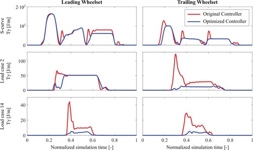
In Figure 8, three examples are selected to showcase the differences between the original feedforward controller and the optimised one in terms of wear number. Concerning the s-curve (Figure 8(Top)), it is possible to see how the optimised controller effectively reduces the wear number in the entering transition curve regions. The same can be observed for the leading wheelset of the second load case (Figure 8(Centre-left)). The difference in the circular curve wear number between the two controllers is negligible since both require the maximum allowable actuation force of 40 kN. In the remaining case, the optimised controller performs better also in the circular part of the curve, where the actuation force can be optimised with respect to the original feedforward controller. This showcases the possibility of further improving the performance of the mechatronic vehicle with a dedicated optimised controller. Nevertheless, it is important to underline that the optimised command steering force profiles are not generally valid outside the load collective defined in Subsection 3.1.1. In Appendix 2 the optimised variables are shown together with the achieved value of the $O_F$ for the 14 curved load cases. Moreover, it is not guaranteed that the solutions obtained with the current optimisation procedure and parameter initialisation represent the global minimum of the OF function, but they serve the purpose of investigating the possibility of shifting the wheelset steering control problem from a vehicle centred approach to a vehicle-infrastructure centred one.

Figure 8. Difference between original feedforward controller and optimised steering controller in terms of wear number: (Left) leading wheelset, and (Right) trailing wheelset. (Top) S-curve, (Centre) Load case 2 (Table 1), and (Bottom) Load case 14 (Table 1).

4.3. Wear number evaluation and expectations

The energy dissipated by a vehicle negotiating a curve can be used to evaluate the performance of the standard bogie vehicle in comparison to the mechatronic one. With constant vehicle speed for each load case, the energy can simply be calculated as (14) $E=\left({\int }_0^{t_{sim}}{T}_{\gamma }^{\mathrm{Leading}}dt+{\int }_0^{t_{sim}}{T}_{\gamma }^{\mathrm{Trailing}}dt\right)\cdot v=O_F\cdot v,$(14) where $v$ is the vehicle speed in m/s. Due to the difference in the number of axles between the standard vehicle and the mechatronic one, for the standard vehicle, in Equation (13), the energy is calculated considering the leading wheelset of the leading bogie as leading wheelset and the trailing wheelset of the trailing bogie as trailing wheelset.

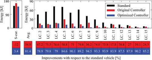
In Figure 9 the values for the dissipated energy are shown for the s-curve and the 14 curve load cases. Both controllers of the mechatronic vehicle are capable of significantly reducing the energy dissipated during curve negotiation. In Figure 9, the improvement achieved by each controller is shown in percentage. As expected, the optimised controller performs significantly better than the original feedforward controller. On average the optimised controller has an improvement of 81.4% against a 54.9% improvement for the original one with a maximum of 93.9% in load case 10 against a maximum of 79.8% in load case 7. These results will be compared in Section 6 with the performance achieved in terms of lost wheel volume. Based on the analysis of the dissipated energy, the mechatronic vehicle is expected to have a significant reduction of the wheel wear, with an even better performance with the optimised controller.

Figure 9. Dissipated energy for the first 15 load cases (the s-curve and the 14 curve load cases) comparing the standard vehicle with the mechatronic one controlled with the original controller and the optimised one. For each load case, the improvement achieved by the mechatronic vehicle with respect to the standard one is given in percentage. The average (Avg.) improvement for both controller is shown too.

5. Results

Results are presented in two sections. In the first, the Archard maps are tuned to fit the measured worn wheels and the comparison with the simulated ones is shown. In the second, the performance of the mechatronic vehicle is evaluated. In these simulations, the Archard maps determined during the first phase are used to guarantee coherence of the achieved results. As per Subsection 4.3, due to the difference in the number of wheelsets of the two compared vehicles, only the leading wheelset of the leading bogie and the trailing wheelset of the trailing bogie are considered for the standard bogie vehicle.

5.1. Validation of experimental results

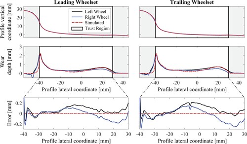
As mentioned in Sub-section 3.2, due to the wayside lubrication, two Archard maps are used to fit the simulated worn wheels to the experimental worn wheels profiles. The maps are automatically selected during the wear calculation in each contact patch. The coefficient of friction is collected as output of the simulations and the maps are switched accordingly. In Figure 10 the simulated worn wheels are compared with the measured worn wheel profiles. The obtained results approximate the measured wheel profiles sufficiently well, especially in the flange region. Comparing the wear depth, calculated as the difference between the unworn wheel profile and the worn wheel profile in a vertical direction, some differences appear in the tread region and flange root. With reference to Figure 3, the difference in the flange root may be explained by the general lack of contact points between the wheel and the rail considering only new rail profiles in the simulations. Nevertheless, the error (Figure 10(Bottom)) between the simulated wheel wear depth and the measured one lies within an interval of 0.2 mm in the ‘trust region’. The trust region has been identified as the region where abrasive wear is expected. Outside of this region, plastic deformation may occur, which is not captured with Archard’s method.

Figure 10. Comparison of measured and simulated worn wheels at the reprofiling distance of 150,000 km: (Left) leading wheelset, (Right) trailing wheelset. (Top) Wheel profiles, (Centre) wear depth, and (Bottom) error between simulated and measured wear depth.

5.2. Results on mechatronic vehicle configurations

Once the two Archard maps are tuned to reproduce experimental results, the same are used to evaluate the wheel wear of the mechatronic vehicle. In this way, the prediction of the mechatronic vehicle wheel wear can be considered reliable and a proper comparison between the two vehicles can be performed.

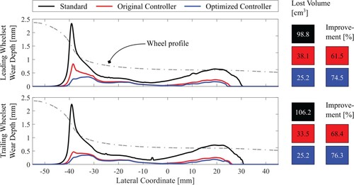
In Figure 11 the wear depth for the considered vehicle configurations is shown for both leading and trailing wheelsets. For coherence of the comparison, for the standard bogie vehicle, the simulated results are used instead of the experimental ones. The mechatronic vehicle performs significantly better than the standard bogie vehicle, with greater improvements when the optimised controller is applied instead of the original feedforward one. Considering the leading wheelset, the flange wear after a running distance of 150,000 km is reduced from approximately 2.3 mm to approximately 0.8 and 0.4 mm using the original controller respectively the optimised one. Tread wear reduces from approximately 0.6 to 0.2 mm, using both control approaches. 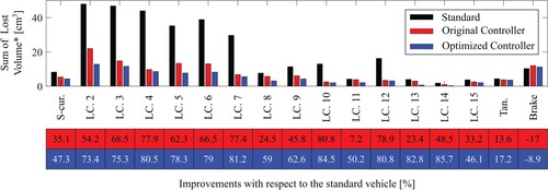An approximate lost volume due to wear can be computed to compare the results, (15) $\mathrm{Lost}\mathrm{Volume}=2\pi r_0{\int }_{y_{in}}^{y_{\mathrm{end}}}{W}_{d}dy,$(15) where $y_{in}$ and $y_{end}$ are the initial respectively final profile lateral coordinates, $W_d$ is the wear depth as function of the lateral wheel coordinate, and $r_0$ is the nominal wheel radius. The lost volume measure of Equation (14) is an estimation of the lost volume since the wheel radius is considered constant and equal to the nominal one. In Figure 11(Right) the lost volume values are shown for the two wheels and the three vehicles. The percentage improvement illustrates the significant reduction that the mechatronic vehicles can achieve, showing a maximum between the two wheels of 68.4% for the mechatronic vehicle controlled with the original controller and 76.3% for the one controlled with the optimised controller.

Figure 11. Wear depth comparison between the standard bogie vehicle and the mechatronic vehicle controlled with the original feedforward controller and the optimised one at the reprofiling distance of 150,000 km. (Left-top) Leading wheelset, (Left-bottom) trailing wheelset. (Right) Lost volume per vehicle and improvements in percentage of the mechatronic vehicles in comparison to the standard one.

A more in-depth analysis can be performed by considering the load cases (Table 1) individually. During the simulations, the normal wear (${\hat{W}}_j\left(y_p\right)$ Equation (3)) is stored separately for each load case, wheel, and wear step. The normal wear for each load case is then recalculated, (16) ${\hat{W}}_j^N=\sum _{k=1}^{N_{\mathrm{steps}}}\frac{1}{2}\left({\hat{W}}_{k,j}^L\left(y_p\right)+{\hat{W}}_{k,j}^R\left(y_p\right)\right)\cdot S_k\cdot \frac{r_j}{L_j^{sim}},$(16) where $N_{\mathrm{steps}}$ is the number of wear steps, ${\hat{W}}_j^N$ is the normal wear for load case j, ${\hat{W}}_{k,j}\left(y_p\right)$ is the normal wear for load case j and wear step k, and $S_k$ is the scale-up for the wear step k. No additional simulations are performed to evaluate the normal wear per load case. Equation (14) can now be applied to ${\hat{W}}_j^N$ to obtain an estimation of the normal volume lost for each load case. In Figure 12, the sum of the two wheelsets lost volume per each load case is shown together with the improvements in terms of percentage. It can be observed that for the very small curve radii load cases (load cases from two to seven) the effect of the steering control is significant, giving a maximum improvement of 77.9% (load case 4) for the original controller and 81.2% (load case 7) for the optimised one, explaining the overall great wear depth reduction shown in Figure 11.

Figure 12. Sum of normal wear lost volume per load case comparing the standard bogie vehicle and the mechatronic one. (Top) Sum of lost volume, (Bottom) improvements with respect to the standard bogie in percentage.

6. Discussion

Mainly two aspects need to be addressed. The first one is the value of the $T\gamma$ function as a tool to preliminary evaluate performances of a vehicle and its effectiveness in the design of new railway systems and steering controllers. The second one concerns the applicability of an optimised on-purpose controller for a specific line in contrast to a more general and always-applicable one.

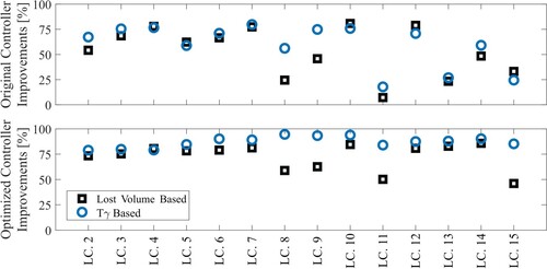
Regarding the first aspect, it is known that global $T\gamma$ based approaches to evaluate wheel wear are generally lacking information about the local stress conditions in the contact patch [8,9]. Nevertheless, being so easy and fast to evaluate, for track scenarios characterised by a high number of curves, the approach can be used as a preliminary tool to design control strategies and evaluate vehicle curving performances. As shown, the improvements achieved with the original and optimised controller obtained with the energy calculation in Subsection 4.3 are coherent with the improvements obtained in terms of lost wheel volume shown in Subsection 5.2. The energy calculation showed greater achievable improvements using the optimised controller and this is reflected in the detailed simulations of the worn wheel volume. With focus on the curve load cases (load case from two to 15), it can be seen in Figure 13 that the $T\gamma$ based (energy calculation) improvements are comparable and sufficiently coherent with the ones based on the lost volume.

Figure 13. Comparison of improvements of the mechatronic vehicle with respect to the standard bogie vehicle calculated with $T\gamma$ based approach (energy calculation) and the ones based on the lost volume. (Top) Original feedforward controller, and (Bottom) optimised controller.

As shown in this study, an optimised on-purpose controller developed for a specific line has the potential to further reduce the wheel wear. Nevertheless, this approach has some disadvantages compared to the general feedforward controller. The first obvious issue is the adaption to a specific track layout which makes it impossible to use the same controller on a different network. This aspect may be less relevant for metro lines (that can be considered as a closed system), but it can be of great importance for other types of rail vehicles. Additionally, the optimised control parameters shown in Appendix 2 are valid only for the load cases used to perform the optimisation. Thus, a more refined optimisation would be needed when the whole track is considered, for instance considering the real configuration of the track itself. More optimisation parameters may be used to take different transition curve types (linear, parabolic or others) and vehicle speed profiles into consideration. This would drastically increase the complexity of the optimisation problem. Moreover, precise information from the infrastructure would be needed, such as location of the vehicle and vehicle speed at any time. A careful evaluation of the benefits that such an optimised controller can bring must be weighed against the complexity of the optimisation requirements and controller reliability.

7. Conclusions

In this paper, the wheel wear evolution of the mechatronic vehicle developed within the Shift2Rail projects Run2Rail, Pivot, NEXTGEAR, and Pivot2 has been evaluated. To increase the reliability of the achieved results, the KTH wear model has been used to tune the Archard wear map coefficients for the standard bogie vehicle S8000 running on Metro Madrid line 10. The same model and coefficients are subsequently used to perform the evaluation of the mechatronic vehicle.

The mechatronic vehicle has been controlled with two different feedforward control steering approaches. The first one was previously developed by the authors while the second one relies on the hypothesis that close communication between the infrastructure and the running vehicle is possible. For the second controller, steering command signals have been optimised with firefly algorithms.

Results show that the controlled vehicle can significantly reduce the lost wheel volume due to wear producing an improvement above 60% and above 70% compared to the current metro vehicles with the original feedforward steering control and the optimised one respectively. Moreover, the effect is more pronounced for the curve sections with very small curve radii (R ≤ 400).

Additionally, sufficient coherence between predicted improvements by $T\gamma$ based (energy calculation) approaches and improvements based on lost volume by wheel wear has been shown. This confirms the possibility of using $T\gamma$ based approaches as a comparative tool for preliminary evaluation vehicle performances.

The benefits introduced by the new mechatronic vehicle prove once more that active steering can be an effective alternative to the standard passive configuration of railway vehicles. Moreover, it shows that feedforward steering approaches are robust solutions that can effectively perform the steering task, regardless of the wheel-rail contact condition. The results also show that a new philosophy of steering control strategies, where vehicle and track have a close communication, can be even more beneficial at the expenses of a more complex system.

Disclosure statement

No potential conflict of interest was reported by the author(s).

Additional information

Funding

This project has received funding from the Shift2Rail Joint Undertaking (JU) under grant agreement No 881807. The JU receives support from the European Union’s Horizon 2020 research and innovation programme and the Shift2Rail JU members other than the Union.

Notes

1 Depending on the used software conventions, signs of Equation (6) may change. Important is to remember that wear removes material from the wheel.

2 According to the knowledge of the authors, in SIMPACK it is not possible to dynamically change the Kalker’s coefficients scaling. Only one constant scaling is allowed and set at the beginning of the simulation. According to [7], Kalker’s coefficients were obtained for a constant friction of 0.6 and can be simply scaled by a ratio $\mu /0.6$. Polach’s formulation [40] is present in SIMPACK and may be applied but it is generally used for falling friction problems involving high slip velocities. Thus, for the present study the scaling factor is set to a constant value of 0.35/0.6.

Appendices

Appendix 1

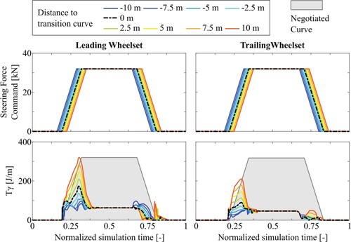
The effect of the command steering force profile timing is showcased here with the second load case from Table 1. The maximum command force is set to approximately 30 kN for both leading and trailing wheelsets. The command steering force profiles have been set to have the same shape of the negotiating curve. The whole command signal for both wheelsets is activated within a specific distance to the start of the entering transition curve. Nine cases are shown in Figure A1, where a negative distance to the transition curve indicates that the command signal is activated before the actual start of the transition curve and a positive one that the command signal is activated after. It can be seen that for the studied case, an anticipation (or preview) of the command steering force is beneficial in terms of wear number in the transition curve area.

Figure A1. Results on preliminary investigation of command steering force profile timing. (Top) Steering force command, (Bottom) energy dissipation $T\gamma$. (Left) Leading wheelset, (Right) trailing wheelset.

Appendix 2

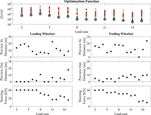
In Figure A2 the results of the optimisation can be seen.

Figure A2. FAs optimisation results for the 14 curve load cases. (Top) $O_F$ for each load case showing the span of the obtained values during the optimisation procedure and the result corresponding to the final optimised value (black circle). (Left) Optimised parameters for the leading wheelset and (Right) the ones for the trailing wheelset.

References

- Fu B, Hossein-Nia S, Stichel S, et al. Study on active wheelset steering from the perspective of wheel wear evolution. Veh Syst Dyn [Internet]. 2020. doi:10.1080/00423114.2020.1838569
- Fu B, Giossi RL, Persson R, et al. Active suspension in railway vehicles: a literature survey. Railw Eng Sci [Internet]. 2020; Available from: https://link.springer.com/10.1007s40534-020-00207-w
- Hur H, Shin Y, Ahn D, et al. Steering performance evaluation of active steering bogie to reduce wheel wear on test line. Int J Precis Eng Manuf [Internet]. 2019;20:1591–1600. doi:10.1007/s12541-019-00167-0
- Tian S, Luo X, Ren L, et al. Active steering control strategy for rail vehicle based on minimum wear number. Veh Syst Dyn [Internet]. 2020;1–26. doi:10.1080/00423114.2020.1743864
- Fu B, Bruni S. Fault tolerant analysis for active steering actuation system applied on conventional bogie vehicle. Int Assoc Veh Syst Dyn. 2019: 90–99. doi:10.1007/978-3-030-38077-9_11
- Giossi RL, Persson R, Stichel S. Improved curving performance of an innovative two-axle vehicle: a reasonable feedforward active steering approach. Veh Syst Dyn [Internet]. 2020;1–24. doi:10.1080/00423114.2020.1823005
- Andersson E, Berg M, Stichel S. Rail vehicle dynamics; 2014.
- Krishna VV, Hossein-Nia S, Casanueva C, et al. Rail RCF damage quantification and comparison for different damage models. Railw Eng Sci [Internet]. 2022;30:23–40. doi:10.1007/s40534-021-00253-y
- Pombo J, Ambrósio J, Pereira M, et al. Development of a wear prediction tool for steel railway wheels using three alternative wear functions. Wear. 2011;271:238–245.
- Jendel T. Prediction of wheel profile wear – comparisons with field measurements. Wear. 2002;253:89–99.
- Enblom R, Berg M. Simulation of railway wheel profile development due to wear influence of disc braking and contact environment. Wear. 2005;258:1055–1063.
- Bruni S, Goodall R, Mei TX, et al. Control and monitoring for railway vehicle dynamics. Veh Syst Dyn [Internet]. 2007;45:743–779. Available from: https://www.tandfonline.com/doi/abs/10.108000423110701426690
- Heckmann A, Schwarz C, Keck A, et al. Nonlinear observer design for guidance and traction of railway vehicles. Adv Dyn Veh Roads Tracks IAVSD 2019 [Internet]. 2020;639–648. Available from: https://link.springer.com/10.1007978-3-030-38077-9_75
- Kaiser I, Strano S, Terzo M, et al. Estimation of the railway equivalent conicity under different contact adhesion levels and with no wheelset sensorization. Veh Syst Dyn [Internet]. 2022. doi:10.1080/00423114.2022.2038383
- Yang X-S. Firefly algorithm, Lévy flights and global optimization. In: Bramer M, Ellis R, Petridis M, editors. Res Dev Intell Syst XXVI Inc Appl Innov Intell Syst XVII [Internet]. London: Springer London; 2010. p. 209–2018. Available from: https://link.springer.com/10.1007978-1-84882-983-1
- Fister I, Yang XS, Brest J. A comprehensive review of firefly algorithms. Swarm Evol Comput. 2013;13:34–46.
- Bevan A, Molyneux-Berry P, Eickhoff B, et al. Development and validation of a wheel wear and rolling contact fatigue damage model. Wear [Internet]. 2013;307:100–111. doi:10.1016/j.wear.2013.08.004
- Hossein Nia S, Casanueva C, Stichel S. Prediction of RCF and wear evolution of iron-ore locomotive wheels. Wear [Internet]. 2015;338–339:62–72. doi:10.1016/j.wear.2015.05.015
- Muhamedsalih Y, Stow J, Bevan A. Use of railway wheel wear and damage prediction tools to improve maintenance efficiency through the use of economic tyre turning. Proc Inst Mech Eng Part F J Rail Rapid Transit. 2019;233:103–117.
- Li Y, Ren Z, Enblom R, et al. Wheel wear prediction on a high-speed train in China. Veh Syst Dyn [Internet]. 2019;3114. doi:10.1080/00423114.2019.1650941
- Muhamedsalih Y, Tucker G, Stow J. Optimisation of wheelset maintenance by using a reduced flange wear wheel profile. Proc Inst Mech Eng Part F J Rail Rapid Transit. 2022;237(2):253–265. doi:10.1177/09544097221105959
- Krishna V V., Hossein-Nia S, Casanueva C, et al. Long term rail surface damage considering maintenance interventions. Wear [Internet]. 2020;460–461:203462. doi:10.1016/j.wear.2020.203462
- Arthur D, Vassilvitskii S. K-means++: the advantages of careful seeding. Proc Annu ACM-SIAM Symp Discret Algorithms. 2007;07-09-Janu:1027–1035.
- Bergander B, Kunnes W. Erri B176/DT 290: B176/3 benchmark problem, results and assessment [tech report]. Eur Rail Res Inst.; 1993.
- Iwnicki S, Spiryagin M, Cole C, et al. Handbook of railway vehicles dynamics. 2nd ed. Broken Sound Parkway NW: Taylor & Francis Group; 2019.
- Run2Rail. Innovative running gear solutions for new dependable, sustainable, intelligent and comfortable rail vehicles, deliverable 3.1 – state of the art actuator technology; 2018.
- Persson R, Stichel S, Liu Z, et al. Cost reduction with single axle running gears in metro trains. Transp Res Arena Conf. 2022: 1–8.
- Run2Rail. Innovative running gear solutions for new dependable, sustainable, intelligent and comfortable rail vehicles, deliverable 3.2 – new actuation systems for conventional vehicles and an innovative concept for a two-axle vehicle; 2019.
- NEXTGEAR. NEXT generation methods, concepts and solutions for the design of robust and sustainable running GEAR, deliverable D2.6 – actuator development.
- NEXTGEAR. NEXT generation methods, concepts and solutions for the design of robust and sustainable running GEAR, deliverable D2.2 – component level demonstrator using fibre reinforced plastic.
- Giossi RL, Shipsha A, Persson R, et al. Active modal control of an innovative two-axle vehicle with composite frame running gear. Proc 27th IAVSD Conf [Internet]. 2022;8–17. Available from: https://link.springer.com/10.1007978-3-031-07305-2_2
- Giossi RL, Shipsha A, Persson R, et al. Towards the realization of an innovative rail vehicle – active ride comfort control. Control Eng Pract. 2022;129:105346. doi:10.1016/j.conengprac.2022.105346
- CEN; EN 12299. Railway applications – ride comfort for passengers – measurement and evaluation; 2009.
- Qazizadeh A, Persson R, Stichel S. On-track tests of active vertical suspension on a passenger train. Veh Syst Dyn [Internet]. 2015;53:798–811. doi:10.1080/00423114.2015.1015429
- Qazizadeh A, Persson R, Stichel S. Preparation and execution of on-track tests with active vertical secondary suspension. Int J Railw Technol [Internet]. 2015;4:29–46. Available from: https://www.ctresources.info/ijrt/paper.html?id=77
- Persson R, Giossi RL, Stichel S. Single axle running gear with nonlinear axle guidance stiffness. Proc 27th IAVSD Conf [Internet]. 2022:355–361. doi:10.1007/978-3-031-07305-2_36
- Zhou GD, Yi TH, Zhang H, et al. A comparative study of genetic and firefly algorithms for sensor placement in structural health monitoring. Shock Vib. 2015;2015:1–10.
- Lunardi WT, Voos H. Comparative study of genetic and discrete firefly algorithm for combinatorial optimization. Proc ACM Symp Appl Comput. 2018:300–308.
- Yang X-S. Firefly Algorithm [Internet]. MATLAB Cent. File Exch. 2022. Available from: https://www.mathworks.com/matlabcentral/fileexchange/29693-firefly-algorithm
- Polach O. Influence of locomotive tractive effort on the forces between wheel and rail. Veh Syst Dyn. 2001;35:7–22.