Development of a Digital Twin for prediction of rail surface damage in heavy haul railway operations

Abstract

Rail surface damage occurs due to repeated overstressing of the surface by wheel-rail contact cycles, which is also known as rolling contact fatigue, and causes regular costly maintenance expenses to railways. The preventive strategies to reduce rail damage can be conservative if it is not based on measured data. A validated digital model of the physical system can provide data for maintenance decision. Interaction between a physical system and a digital model has evolved at the beginning of this century into a new process commonly referred to by the term ‘Digital Twin’. There is a lack of a Digital Twin framework in decision-making on railway maintenance. The term Digital Twin is often confused with advanced simulation methods where the communication of data is only one way, i.e. sensor or design data of the physical system input to a model. In this paper, a Digital Twin has been developed to predict rolling contact fatigue rail surface damage, corresponding to traffic passing along a railway network. Differences between the Digital Twin and advanced simulation techniques have been presented. Finally, a predictive assessment tool has been proposed to provide prediction from the Digital Twin to the physical twin, and results are discussed.

Abbreviations: AS: Advanced Simulations; DS: Digital Shadow; DT: Digital Twin; HPC: High Performance Computing; LTS: Longitudinal Train Simulation; MBS: Multibody Simulation; MGT: Million Gross Tonnes; NASA: National Aeronautics and Space Administration; RCF: Rolling Contact Fatigue

KEYWORDS:

• Digital Twin
• rolling contact fatigue
• predictive maintenance
• advanced simulation
• rail wear

1. Introduction

Rail surface damage occurs due to repeated overstressing of the surface by wheel-rail contact load cycles [1]. The damage due to repeated wheel-rail contact is known as Rolling Contact Fatigue (RCF). Heavy haul rail lines face more RCF due to the consistency of speed, load, and uni-directional loaded train travel which results in regular repeated load cycles on the rails. RCF has been considered a dominant reason for rail replacement, maintenance, rail failure, and safety concerns [1]. Due to the high cost involved in rail replacement and failure, preventive rail grinding is used in railways which may also be conservative. To find a solution to the RCF problem and management, rail and wheel wear models have been extensively studied [2–7]. Researchers often use empirical relationships and engineering assessments to obtain an estimation of wear on rail and wheels [3,8]. The experimental estimation of rail wear often involved a controlled experiment with twin discs of equivalent wheel and rail geometry [2].

The rail surface damage depends on contact geometry between wheel and rail which is nearly impossible to measure during operation because of the inaccessibility of the contact zone by a physical sensor. Multibody simulation allows estimating the contact patch area using theories such as a fast algorithm for a simplified theory of rolling contact, modified Fastsim, or extended contact algorithm [9–11].

With the advent of improved computing power, digitisation, and model-based system engineering, the use of virtual product models has increased [12]. The virtual model can coexist and interact with the physical system over the whole life cycle of the product- design, manufacturing, usage, and service [13]. The virtual model that can communicate with its physical system is regarded as the Digital Twin (DT) of the physical product.

The concept of DT has gained popularity recently in the field of railway engineering [14–16]. However, there is a lack of a framework in applying a DT to the advancement of rail vehicle simulations. A review of what constitutes a DT and application of DT in rail vehicle simulation has been performed in this paper. In this paper, a DT has been developed to provide rail surface damage indications along a railway route. The model representing the situation more realistically by using the co-simulation approach between the train and individual wagon is in this article referred to as a Digital Twin (DT) as distinct from the other models Advanced Simulation (AS) and Digital Shadow (DS), although all the models compared here could serve as the basis for a DT. The DT developed in this paper uses advancements in simulation techniques in Longitudinal Train Simulation (LTS), Multibody Simulation (MBS), and Co-simulation between simulation environments (including power traction system simulations in Matlab/Simulink) that allows creating a more precise digital world replica of a physical system. The proposed DT combines both model-driven and data-driven approaches. The differences between a DT compared with either an AS or a DS have been explained with a case study. Finally, an example case of using a DT for prediction of Rolling contact fatigue (RCF) data on a rail along the track has been presented and the results are discussed.

1.1. DT characteristics

The National Aeronautics and Space Administration (NASA) believed that the DT was a kind of simulation of a vehicle or system by using the best available physics-based models, sensor updates, and fleet history to depict the states of the flying twin [17]. Glaessgen and Stargel defined the DT as an integrated multi-physics, multiscale, probabilistic simulation of a complex product, which functions to mirror the life of its corresponding twin [18]. A DT is not only representing the standalone model but also focuses on the bilateral interdependency of the virtual and physical representations. This two-way communication between the physical model and the DT in real-time ensures interactive maintenance during the operational activities and can adapt to modify the DT accordingly. Schleich et al. [12] explained two-way communication as twinning between a physical system and a corresponding digital system by observation and prediction respectively. The information transfer from the physical system to the digital system would be by sensors and observation. The prediction from the digital system to the physical system relies on scientific assumptions, simulations, virtual testing of models, and consideration of uncertainty for certain characteristics [12].

The use of a DT can provide ideas for vehicle development, intelligent operation and maintenance of infrastructure, a virtual test of unmanned driving, and live traffic analysis [19]. Tao suggested that a DT should consist of five dimensions, namely physical objects, virtual models, data, services, and the connections between them [20]. Most researchers agreed that a high-fidelity model and real-time interaction between physical and virtual spaces are the main features of a DT [13,21,22].

One of the benefits of the DT is regarded as deciding on undertaking maintenance based on technical conditions rather than regular preventive measures [23]. This would lead to predictive maintenance which would determine the maintenance schedule when it is necessary rather than relying on routine maintenance [24]. A data-driven approach to manage track maintenance was proposed in [25]. The data-driven system relies on near real-time monitoring of track by track-recording cars. The data obtained by sensors need to be pre-processed to train a machine-learning algorithm to use for predictive maintenance [24]. The data in the server can be compared with a reference point to achieve a desired outcome to be applied as input to a physical system [26].

A data-driven approach needs big data which must be sourced from physical sensors or digital simulation. There is a limitation on physical sensor data as not all parameters can be obtained physically. To overcome this shortage of sensor data, a digital model of the physical system can be used to generate additional sensor data that can be used for predictive maintenance. The use of a digital model is also useful to test various severe conditions that are not possible to test in a regular operation.

Wright and Davidson [27] identified three important parts of the DT of an object based on definitions of various sources, namely a model of the object, an evolving data set relating to the object, and a means of dynamically updating the model based on that data. It was also noted that a DT must have a corresponding physical object. Without the physical object, the DT would be considered just a model. DTs for design can be implemented at the prototype stage where test data from the prototype can be used to update the parameters in the digital model. The results from the digital model, engineering understanding, and previous experience can be used to predict the performance of the physical model. The process of improvement in design can continue by doing extra iterations in a controlled environment.

In the case of high-value engineering applications, the success of prediction by the DT would require a system that can input supplier data, in-house testing results, and online and offline measurement results into a DT of a product [27]. Depending on the accuracy of the model and data, the DT of the product can supply rapid performance predictions.

Schwarz and Wang [28] identified that the presence of communication is a key differentiator between DTs and models. Three terminologies were introduced – digital model, digital shadow, and DT. A digital model represents an equivalent characteristic of a physical model but does not provide any communication or data exchange between physical and digital products. In the digital shadow, data is only transferred one-way from the physical to the digital system. In the DT, data are exchanged in both directions.

Application of a DT is useful if there is a change in parameters during operation such as wear in machinery influencing performance [27]. A DT is applied not only during conceptualisation, prototyping, testing, and optimisation phases, but also during the operational phase so as to encompass the complete product life cycle and beyond to improve performances throughout the lifecycle and disposal of a product [26]. At the operational stage, the success of the DT depends on the availability of real-time data from the physical system.

1.2. DT in rail vehicle simulation

Krishna et al. [14] proposed a method to calculate long-term rail surface damage using a 1-D longitudinal train simulation and a 3D multibody simulation of multiple vehicles in parallel. To reduce the modelling effort, the authors opted to model the first locomotive and four equally placed wagons in the train to obtain a reasonable approximation of wear over the whole train. A weighting of wear based on results of wear on locomotives and wagons was used to scale the wear limit corresponding to the tonnage passed. It was proposed that the rail profiles be updated by taking into consideration the wear and RCF at every time step. The rail profile would also be updated when a grinding interval was reached. The grinding operation would add grind profile depths on top of the vehicle-induced wear depth. In addition to that, the grinding application would remove cracks which would require resetting the RCF to zero. The method proposed by Krishna et al. [14] uses the LTS data (acting forces and kinematic state variables on each vehicle) as an input and then runs MBS on selective track sections using the inputs from LTS. This method can be considered as an advanced simulation technique as LTS and MBS were run separately and no communication between the model and physical system was formulated.

Sun et al. [15] proposed a DT approach by using a multibody model of a train that had 11 multi-body wagon models connected with a longitudinal coupler model. However, communication between the numerical modelling and the physical train operational environment was not provided, hence the method does not fulfil the DT criteria. However, as it used data from the physical track structure, it fulfils the definition of the digital shadow approach.

Using advanced simulation models of locomotives, track and traction, a method has been presented in [16] to perform shakedown analysis of rails. Advanced simulation approaches such as variable wheel-rail frictions, including locomotive traction mechatronic system using co-simulation between MBS and Simulink were implemented in [16]. In the simulation approach in [16], the train operational data, field measurements, and experimental data were added as inputs to the advanced numerical model of the locomotive. Post-processing was performed to present a shakedown analysis for the variety of operating conditions on a 240 m section of track. A variety of notch conditions (1–8) were used at two speeds (20 and 70 km/h) travelling over both tangent and curved track to generate 48 simulation studies. It follows that a large number of simulation cases would be required considering a wide range of measured and operational conditions for a wear prediction tool.

The literature review on rail vehicle simulation showed that a framework to separate the ‘DT’ term from advanced simulation techniques is lacking.

2. Methodology

A methodology to develop a DT to predict rail surface damage has been presented in Figure 1. The starting point of the development of the DT would be taking initial inputs from a physical system. In the case of a rail surface damage study, the physical system would generate parameters of train configuration and driving commands, vehicle parameters (locomotives and wagons), track geometry, plus wheel and rail profiles.

Figure 1. Methodology to develop a DT for prediction of rail surface damage.

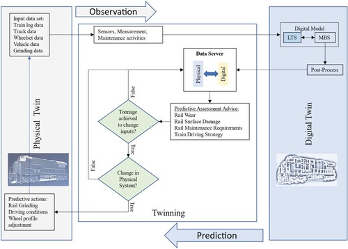
The inputs of the physical twin would be added in a DT. In the case of train simulation, the digital model would consist of train and individual vehicle models. The train modelling considers longitudinal train dynamics whereas the individual vehicle models would consider detailed 3D modelling of each vehicle including their suspension models, track irregularity parameters, and wheel-rail contact to represent the actual vehicle dynamics in a digital model. Longitudinal train simulation provides coupler forces (longitudinal and lateral), plus speed and notch (driving command) information.

A detailed modelling of vehicle components including wheel and rail contact is necessary for evaluating rail surface damage which can be implemented in an MBS tool. It can be noted that LTS does not explicitly include wheel and rail contact models which means the resistance equation in LTS does not consider the friction forces on the wheel and rail contact. As a result the LTS provides a simplistic resistance values to vehicles compared to MBS and resulted in variation in speed, and position of vehicles compared to that obtained in MBS. In an advanced simulation method, the two different software LTS and MBS packages were connected using a TCP/IP interface to synchronise speed, the position of vehicles, and realised traction effort on vehicles on LTS and MBS [29].

It is necessary to provide feedback to the physical system to fulfil the requirement of a DT. It is proposed that the results of the MBS system would be stored in a data server that would provide predictive feedback to the physical system using a predictive assessment advice tool.

In this paper, a method has been developed to use the RCF results in the data server in a predictive analysis tool to assist predictive management of RCF. An example to implement grinding cycles based on RCF damage has been demonstrated.

2.1. Parameters for RCF Study

The study of rail wear is often based on a parameter called wear number expressed in [8] as the term Tgamma (Tγ) which is defined as the sum of the product of traction forces and creepages (longitudinal and lateral) at the contact patches. In a later study, it was found that the angular creepage or spin creepage on wheel and rail contact patches affect the RCF significantly in the flange of the wheel and the gauge corner of the rail [30]. Hence, in this paper, the Tgamma calculation uses longitudinal, lateral, and spin creepage (Equation (1)) [31]. (1) $\begin{array}{r}{\mathit{T}}_{\mathit{\gamma }}={\mathit{T}}_{\mathit{x}}{\mathit{\gamma }}_{\mathit{x}}+{\mathit{T}}_{\mathit{y}}{\mathit{\gamma }}_{\mathit{y}}+{\mathit{M}}_{\mathit{s}}{\mathit{\gamma }}_{\mathit{s}}\end{array}$(1) where $T_{\gamma }$ is the energy dissipated at the contact also presented as Tgamma (Nm/m), $T_x$ is the longitudinal creep force (N), $T_y$ is the lateral creep force (N), $M_s$ is the spin moment (Nm), ${\gamma }_x$ is the longitudinal creepage (m/m), ${\gamma }_y$ is the lateral creepage (m/m), ${\gamma }_s$ is the spin creepage (1/m).

Rail surface damage can be calculated using two methods, namely Fatigue Index by Shakedown Map [32,33] and Rolling Contact Fatigue Index by Tgamma [8]. In this study the RCF index by the Tgamma method has been used to demonstrate the application of the DT.

A piece-wise-linear model approach correlating RCF and wear with Tgamma, originally developed by RSSB UK in [8] and subsequently modified for hardened rail (Figure 2) in [34] has been used in this paper. For a hardened rail (example, R370CrHT), the RCF damage will not occur until the Tgamma value of 38 (Figure 2). RCF damage will dominate when the Tgamma value is between 38 and 65. The probability of RCF damage decreases and wear increases when Tgamma is above 65. Severe wear would be expected when Tgamma is above 200.

Figure 2. The RCF damage index function [34].

Knowing the average RCF index for a wheel over a track section, it will be possible to estimate the number of load cycles that can create a visible RCF (Equation (2)) [8]. (2) $\begin{array}{r}\text{RCF}=\frac{1}{{\mathit{N}}_{\mathit{f}}}\end{array}$(2) where RCF is the fatigue damage index in 10⁻⁶, N_f is the number of cycles to failure.

2.2. Post-processing of results

The results obtained from MBS need to be stored in a suitable format for future use. In this paper, the data were stored in *.mat format. Post-processing was performed to obtain moving averages of RCF over every 40 m distance along the route.

2.3. Predictive assessment

The data stored in the data server can be used as required to assess a predictive action plan. A field measurement method provided by Innotrack [35] identified four levels of damage based on wear and RCF damage per 100 Million Gross Tonnes (MGT) of passing traffic as shown in Table 1. The damage index obtained by simulation gives a level of severity of damage that is different from the physical understanding of wear mechanisms. The damage index in the simulation tool calculates the energy dissipated on the contact patches and compares it with physical data to establish a relationship between the damage index and measured wear. Physically, wear cannot be measured unless it is visible, but the damage index provides a probability of damage levels that cannot be measured physically. Hence, the damage index tool can be used as a predictive analysis tool.

Table 1. Severity of RCF damage index.

		Equivalent RCF damage index for 100 MGT, (dimensionless, in 10^−6)
Level of damage	RCF crack depth per 100 MGT [35] (mm)	Normal rail grade	Premium rail grade
Light	< 0.5	2.5	0.74
Medium	≤ 1	5	1.485
Heavy	≤ 3	15	4.455
Severe	> 3	15	4.455

In a simulation, RCF parameters are reported as indexes rather than crack size. The approximation suggested by AEA Technology, RSSB, UK [8] states that RCF will be visible (crack size of 2 mm [36]) when the value of the RCF damage index reaches 10 × 10⁻⁶. For a hardened rail, the RCF damage index for a visible crack (2 mm) would be 2.97 × 10⁻⁶ (Figure 2). Hence, it can be approximated that, to generate 1 mm of crack, the RCF index would be 5 × 10⁻⁶ and 1.485 × 10⁻⁶ for normal grade and premium grade rails respectively. Following this, the RCF index for different levels of damage for over 100 MGT of passing traffic can be estimated by multiplying the crack depth by 5 and 1.485 for normal grade and premium grade rails respectively. In this paper, the data for premium rail grade has been used.

3. Differences between advanced simulation, digital shadow, and DT

The differences between the AS, DS, and DT can be explained using the frameworks of AS, DS, and DT presented in Figure 3.

Figure 3. Frameworks of AS, DS, and DT.

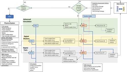
In the Advanced Simulation (AS) method, the LTS was run for the complete length of the track section over which the train was being simulated using actual inputs from an operational physical system. The LTS input includes track curvature, track gradient, locomotive traction characteristics, train configuration, and the mass and length parameters of locomotives and wagons. The train driving commands can be taken from a physical log of a train operation or by following a train driving strategy. The outputs from LTS include coupler forces, train speed, and location of vehicles. The output parameters of the LTS were saved in a timeseries which would be used as an input to the MBS. A co-simulation approach was used to implement the traction characteristics in the MBS. The outputs from the MBS can be manually post-processed to perform an analytical analysis.

In the DS method, the outputs from the LTS are directly added to the MBS. An analytical analysis would subsequently be performed manually on the results from the MBS.

In the DT method, LTS and MBS communicate with each other in both directions to update the track position and the realised tractive effort based on wheel-rail friction and traction characteristics in the traction model.

4. Model parameters

A hypothetical case study has been used to demonstrate the application of different simulation methods to apply predictive maintenance guidelines. Three software packages were incorporated in this paper to simulate locomotive behaviour in a train namely LTS, MBS, and traction modelling in Simulink code generation.

4.1. Longitudinal train simulation

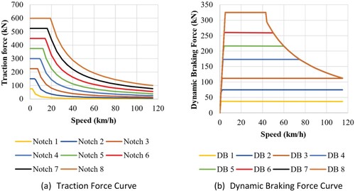
The longitudinal train simulation was performed using an in-house LTS software [31]. The LTS uses a single degree of freedom model to estimate train resistance (rolling, curving, and gradient resistance) using empirical functions [37]. It can be noted that air resistance part of the train resistance has not been added in this study to represent a simplified case for demonstration purpose. Locomotive traction and dynamic brake forces were calculated using a lookup table generated from the traction characteristics curve of the locomotive (Figure 4). The LTS provides speed data based on resistance along the track and the driving commands given to the locomotives.

Figure 4. Traction and dynamic braking force characteristics of the locomotive.

The train consists of 4 locomotives and 160 wagons. The locomotives were placed with two at the front, then 106 fully loaded wagons, then two locomotives, and 54 fully loaded wagons. The locomotives have a mass of 136 t each, and the loaded wagons are 92 t each which makes the total train mass of 15,264 t. The maximum tractive effort of the locomotives is 600 kN each.

The lateral and longitudinal coupler forces were recorded for all vehicles in the train simulation. Each vehicle has front and rear couplers. The lateral force on the couplers was calculated for all wagons using equations for coupler angles provided in the LTS [31] and applied as an external force on the front and rear couplers of vehicles in MBS. The longitudinal force on the front and rear coupler provides a longitudinal force on a vehicle which was applied on the wagon body in the multibody model in this paper. The force component applied to each vehicle was calculated in accordance with Equation (3). (3) $\begin{array}{r}{\mathit{F}}_{\mathit{L}\mathit{o}\mathit{n}\mathit{g}}=\mathit{F}{\mathit{c}}_{\mathit{r}\mathit{e}\mathit{a}\mathit{r}}-\mathit{F}{\mathit{c}}_{\mathit{f}\mathit{r}\mathit{o}\mathit{n}\mathit{t}}\end{array}$(3) where F_long is the longitudinal force from couplers on a vehicle (N), $F{c}_{rear}$ is the longitudinal coupler force on the rear coupler of a vehicle (N), $F{c}_{front}$ is the longitudinal coupler force on the front of a vehicle (N).

In Equation (3), a positive value of longitudinal force means that the rear coupler force is higher than the front coupler force which puts the vehicle into compression. The negative value of $F_{Long}$ would mean that that vehicle is in tension or that a pulling force is applied on the vehicle.

4.2. Multibody simulation

The multibody model of the locomotive was modelled in GENSYS multibody simulation software [38]. A validated multibody model used in [16] has been used in this paper. The validation was based on simulation-based tests as per Australian Standard AS7509 [39] and the locomotive model acceptance procedure [40,41]. The model parameters are listed in Table 2.

Table 2. Multibody model parameters of the locomotive.

	Parameter	Unit	Value
Dimensions	Length over couplers	m	21
	Nominal coupler height above rail level	m	0.89
	Bogie pivot longitudinal distance from wagon body CoG	m	6.85
	Bogie semi-wheelbase	m	1.9
	New wheel diameter	m	1.066
	Total mass	kg	136200
Car-body	CoG height above rail level	m	1.93
	Mass	kg	92614
	Moment of inertia, roll	kg.m^2	143503
	Moment of inertia, pitch	kg.m^2	3535905
	Moment of inertia, yaw	kg.m^2	3545078
	Floor level	m	1.5
Bogie frames	CoG height above rail level	m	0.733
	Mass	kg	11912
	Moment of inertia, roll	kg.m^2	5431
	Moment of inertia, pitch	kg.m^2	29507
	Moment of inertia, yaw	kg.m^2	34045
Wheel sets	CoG height above rail level = New wheel radius	M	0.533
	Mass	kg	3,293
	Moment of inertia, roll	kg.m^2	1526
	Moment of inertia, pitch	kg.m^2	385
	Moment of inertial, yaw	Kg.m^2	1534
Wheel- rail	Wheel profile		New ANZR1
	Rail profile		New AS60
	Wheel-rail contact		Modified Fastsim
	Coefficient of friction at wheel-rail contact		Variable
Secondary suspension	Rubber springs		4 elements on each bogie
	Longitudinal and lateral shear stiffness	kN/m	188.4
	Vertical stiffness	MN/m	7.9
	Traction rods		2 elements on each bogie
	Stiffness	MN/m	5
	Damping coefficient	kN.s/m	20
	Yaw viscous dampers		2 elements on each bogie
	Damping coefficient	kN.s	120
	Lateral bumpstop between wagon body and bogie frame [a]		One element on each bogie frame
	Break points	mm	30, 40, 90
	Stiffness at the break points	kN/m	0, 15, 2000
	Vertical bumpstop between wagon body and bogie frame [a]		Two elements on each bogie frame
	Breakpoints	mm	25, 30, 80
	Stiffness at the breakpoints	kN/m	0, 15, 2000
	Lateral viscous damper (asymmetrical)		Two elements on each bogie frame
	Damping coefficient	kN.s/m	40
	Longitudinal viscous damper (asymmetrical)		Two elements on each bogie frame
	Damping coefficient	kN.s/m	40
Primary suspension	Primary Coil springs [b]		6 elements on each bogie
	Longitudinal shear stiffness	MN/m	3, 45, 45
	Lateral shear stiffness	MN/m	2.5, 1.25, 1.25
	Vertical stiffness	MN/m	0.76, 0.76, 0.76
	Primary damper [b]
	Longitudinal damping coefficient	kNs/m	35, 3.5, 3.5
	Lateral damping coefficient	kNs/m	20, 20, 20
	Vertical damping coefficient	kNs/m	20, 20, 20
	Primary Longitudinal bumpstop		3 elements on each bogie
	Distance to hardstop	mm	50
	Stiffness at hardstop	MN/m	40
	Primary Lateral bumpstop [b]		3 elements on each bogie
	Stage 1 distances	mm	20, 8.75, 8.75
	Stage 2 distances	mm	21, 20, 20
	Stage 3 distances	mm	50, 21, 20
	Stage 1 stiffness	MN/m	0, 0, 0
	Stage 2 stiffness	MN/m	1, 0.028, 0.028
	Stage 3 stiffness	MN/m	2, 1, 1
	Vertical bumpstop [b]		6 elements on each bogie
	Breakpoints	mm	25, 50
	Stiffness at breakpoints	MN/m	0, 1

Note: [a] Multi-stage elements, [b] Three values on each parameter set represent the three wheelsets of a bogie, the parameter values are expressed for the first, second, and third wheelset of a bogie.

The locomotive model consists of 1 car body, 2 bogie frames, and 6 wheelsets. The bogie frame is of bolsterless configuration. Each bogie has three wheelsets each in a Co–Co arrangement. A two-stage suspension system has been added to the bogie frame providing primary and secondary suspensions. Both stages of suspension comprise vertical and lateral damping elements and the secondary suspension also has yaw dampers.

Measured data of wheel and rail profiles were used in this study. The wheel-rail contact model was modelled using the ‘creep_contact_1’ element in GENSYS [42] that uses Kalker’s detailed rolling contact library [43]. The ‘creep_contact_1’ element in GENSYS allows up to 7 points of contact simultaneously for each wheel-rail contact patch.

Friction coefficients and friction model parameters are introduced individually for each contact patch on all wheels. Friction coefficients were varied based on longitudinal creepage following the method proposed by Polach [44]. The maximum friction coefficient at the wheel-rail contact was considered as 0.44.

The multibody model shares data with the LTS model via a TCP/IP server in both DS and DT [31]. The traction behaviour in the MBS model was applied using a sky-hook element as implemented in [45].

4.3. Traction model

The traction model was implemented in a code-generated environment and a co-simulation approach has been implemented to connect the MBS model and the traction model [46,47]. The modelling approach combining MBS with a code generated platform in Simulink using TCP/IP communication is considered an advanced simulation as it considers a detailed electro-mechanical model of the locomotive [46].

The tractive and braking forces were applied as torques to the wheelsets while the resistance forces were applied to the vehicle body. In this paper, the multibody simulation of only the front vehicle (the leading locomotive) was performed for simplicity. As the front vehicle is considered only, the force component applied is much higher than for trailing vehicles which would give higher forces applied by the front vehicle and produce more wear damage than the trailing vehicles. It can also be noted that, as only one simulation case was performed, it is assumed that the contact points remain at the same point for the duration of train passes which would not be the case in actual operation. This simple case is used as it takes less computational effort and is adequate to identify differences between the simulation methods in this paper.

5. Results

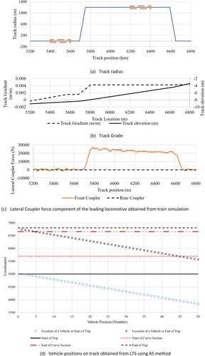
To test the various approaches proposed in this paper, a simulation was run between track position kilometrages of 5 and 6.7 km on a track section which has a right-hand curved track section of 1200 m radius between 5.69 and 6.65 km (Figure 5(a)).

Figure 5. Track data and lateral coupler force data obtained from train simulation.

5.1. Simulation time

It was found that the advanced simulation method was faster (49727s or 13.8 h) than the DS (52192s or 14.5 h) and the DT (59402s or 16.5 h) methods based on a simulation run over the 1.7 km track section distance. The only difference among the models was the communication between MBS and LTS. Hence, it can be identified that on the DS and DT the increased time was spent on communication between the LTS and MBS tools. In the DS, the communication was only in one direction, but in the DT the communication was in two directions which made the simulation time of the DT longer than that of the DS.

5.2. Results of LTS

The track inputs were obtained from an actual heavy haul track with typical curves and gradients (Figure 5). The driving commands were given by manually setting notches at different time intervals to run the train over the chosen track. To demonstrate the method, notch was gradually increased to 8 between 5 and 5.03 km and remained at 8 on the test section. The inputs used for LTS were kept the same for all three methods tested in this paper.

To demonstrate the method, one straight (5400–5600 m) and one curved section (6200–6400 m) were considered. In AS, the train simulation was performed over the entire track but, in DS and DT, train simulation stopped when MBS stopped at 6.8 km. AS MBS was modelled for the front locomotive only, it is understood that the first locomotive of the train reaches to 6.8 km mark but the trailing vehicles were behind the 6.8 km mark as can be seen from location of all vehicles at the start and end of trip from LTS (Figure 5(d)). Vehicle number 44 just reached to curved track (5690 m) and vehicle number 73 entered the starting position of simulation (5000 m) at the end of simulation run. For a full train analysis, all wagons need to pass the test section which was not performed in this paper due to the high computation time requirements.

The leading locomotive (vehicle number 1, Figure 6(a)) experiences much higher propulsion forces (3600–4900 N) compared to trailing wagons (1000–1500 N). Propulsion resistance (running resistance) progressively increases over the time period of simulation (Figure 6(b)). The maximum and minimum curving resistance corresponding to vehicle positions are shown in Figure 6(c). Vehicle number 1 showed the maximum curving resistance of 690N (red circle in Figure 6(c)). Curving resistance is zero on the straight track section which means that some of the wagons which have not negotiated the curve section would still be on the straight section and would not provide any curving resistance. Up to the 44th vehicle of the train has just entered the curved section (at position 5690 m, Figure 5(d)), which would produce some curve resistance force on the respective wagons (Figure 6(c)). Leading Locomotives and wagons provided much more curve resistance (700N) than the trailing wagons (150N), Figure 6(d). Like the curve resistance, the grade resistance was calculated only up to 44th vehicle as the full train did not pass the test section during the example run (Figure 6(e)). The leading locomotive and wagon provided higher grade resistance (−2600 to 5600N) compared to trailing wagons (−1700 to 3800N), Figure 6(f).

Figure 6. Resistance forces and longitudinal coupler forces on Train obtained from LTS.

Note: W1 refers to leading group of wagons, i.e. vehicle number 3-108.

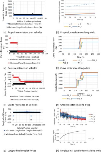
The train simulation in the example AS case showed that the $F_{Long}$ force is significantly larger on locomotives compared to that on wagons (Figure 6(g)). The longitudinal coupler force on the locomotives were between 200 and 435 kN (vehicle positions 1,2, 108 and 109, Figure 6(g)). In wagons, $F_{Long}$ varies between −13 and 36 kN at vehicle positions 81–85 which are in the middle of the train (Figure 6(g)). The variation of longitudinal coupler forces along the trip is high in locomotive compared to wagons (Figure 6(h)).

In the AS method, the speed profile obtained from LTS was applied as input to the MBS. But, in the DS and DT methods, speed data was obtained by one-way communication from LTS to MBS in the DS and two-way communication in the DT (Figure 7). The speed profiles of AS and DS methods match as the LTS conditions were the same in both. The speed by the DT method was found to be lesser than that obtained in both AS and DS (Figure 7). In the DT method, the LTS modifies the speed, vehicle positions, and the realised tractive effort calculated in the MBS.

Figure 7. Traction force characteristics and train speeds in MBS and LTS.

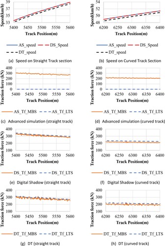
In the AS method, no communication was made with the LTS, and the traction force element in the corresponding LTS method was not stored and was set as zero (Figure 7(c,d)). In the DS method, traction forces obtained in the LTS are higher than those obtained in the MBS (Figure 7(e,f)). In the LTS, the losses in non-linear elements of the vehicle including wheel-rail friction are not considered which has resulted in higher traction forces in the LTS. In the DT method, the realised traction effort calculated in MBS has been transferred to the LTS which updated the latter’s traction forces. Thus, in the DT method, the LTS provides a realistic traction force compared to that obtained in the DS method (Figure 7(g,h)).

5.3. Results of MBS

Two main parameters that are required for the predictive tool in this paper are Tgamma and RCF. Tgamma values were obtained at the 7 simultaneous contact points available on each wheel-rail contact in MBS which were summed to obtain Tgamma on that point. In a post-processing script, RCF values were calculated corresponding to Tgamma for premier rail grade using the piece-wise-linear model in Figure 2. The RCF values were further averaged over a 40 m distance.

5.3.1. Tgamma

The Tgamma values of all wheels on both straight and curved sections were found to vary among the wheel positions (Figure 8). On the straight track section, wheel number 112 l (second wheelset of the first bogie on the left side) produced the largest Tgamma on the left rail (Figure 8(a)) while wheel number 113r (third wheelset of the first bogie on the right side) produced the largest Tgamma on the right rail (Figure 8(b)). The wheels that produced the largest Tgamma on the curved section are 111 l on the high rail and 123r on the low rail respectively (Figure 8(c,d)).

Figure 8. Tgamma of all wheels on straight and curved sections.

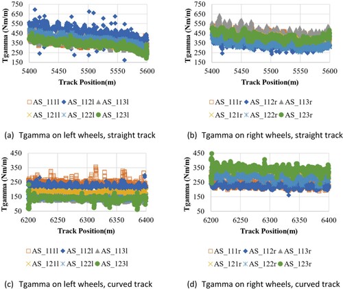
Tgamma values increase with the increase of traction force as can be seen from the result of the straight track section (Figures 7 and 8). On the curved track section, the traction force component was much lower compared to that on the straight track section which resulted in reduced Tgamma on the curved section (Figures 7 and 8).

The average values of Tgamma of the six wheels on each rail showed a small variation among the AS, DS and DT methods (Figure 9(a,b)). A linear relationship between Tgamma and traction force was achieved on the left rail on the straight track (Figure 9(c)). However, the Tgamma values on the right rails were dispersed over a wider range (Figure 9(d)).

Figure 9. Effect of Traction force on Tgamma – straight and curved track sections.

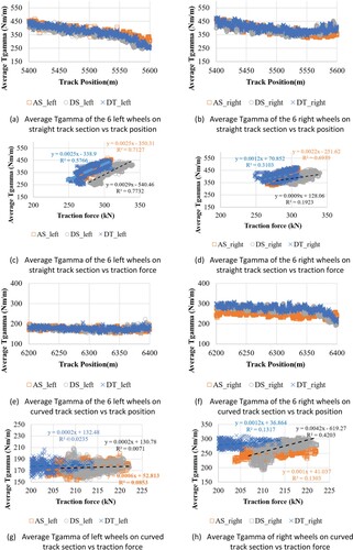
The Tgamma values obtained by the DS method have been found to be less compared to those found by AS and DT methods at the same traction force levels (Figure 9(c,d)). This is because the traction force component in the DS method was obtained by LTS which is higher than the realised traction force in MBS (Figure 9(c,d)). In MBS, the Tgamma value was estimated for the realised traction force component. As the DS method does not have feedback from MBS to LTS, the traction force component does not get corrected during simulation. In contrast, the DT method updates the traction force based on the MBS model which allows a better prediction of the Tgamma based traction force in DT.

On the curved section, the traction force did not vary much, which did not provide an adequate data sample to establish a relationship between traction force and Tgamma values (Figure 9(e–h)).

5.3.2. RCF

Following the method used in Tgamma analysis, RCF data averaged over 40 m distance were further averaged on the left and right wheels. On the straight track section, all RCF values were negative (Figure 10(a)) which means that wear damage is more probable rather than RCF damage considering Tgamma values were above 68 on the track section (Figures 8 and 9). The traction force was much higher on the straight track than on the curved section (Figure 7) which led to a more wear-prone condition rather than RCF damage on the straight track.

Figure 10. RCF values (average of 6 wheels on left and right rails) using advanced simulation approach.

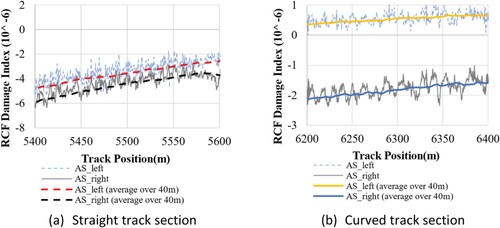
On the curved track, the left rail (i.e. high rail on the right-handed curve) showed positive RCF values (less wear) but the right rail showed negative RCF (more wear) (Figure 10(b)). Due to a slow speed on the curved track (49–51 km/h on a 1200 m radius track with a cant of 65 mm) the vehicle was operating in excess cant conditions (cant excess of 39–41 mm on a standard gauge track following the relationship on a standard gauge track, E = 11.82*V²/R, where E = C + Cd, is the equilibrium cant in mm, C is the applied cant in mm, Cd is the cant deficiency in mm, V is the speed in km/h and R is the track radius in m, negative value of Cd would mean a cant excess condition [48]) on the curve which added more vertical force on the low rail and hence more wear on the low rail. This result agrees with the observation found in an FRA document [49].

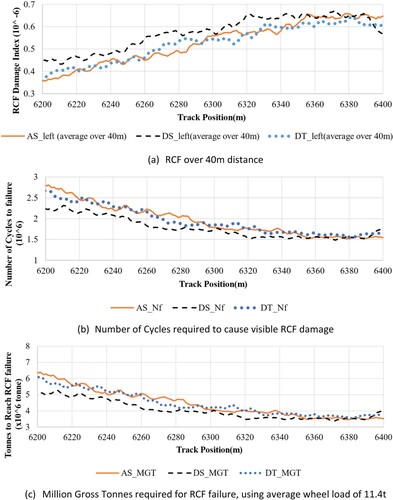
The left rail on the curved section has been further used to quantify the loading cycles (Equation (2)) and million gross tonnes required to cause the RCF failure (Figure 11). Of the three methods implemented in this paper, the DS method gives higher RCF values (therefore less load cycles and MGT to failure) compared to the AS and DT methods (Figure 11).

Figure 11. RCF failure prediction on left rail on the curved section.

6. Predictive maintenance tool

Using the results of the DT method (Figure 11), on the left rail on the curved section (6200 m) the RCF would be 0.374 × 10⁻⁶ which corresponds to 6.08MGT of load. At the 100MGT mark for the same load, the RCF damage accumulation would be 0.374*100/6.08 = 6.15 × 10⁻⁶ which can be classified as ‘severe’ based on Table 1.

It can be noted that the RCF in this paper was calculated for a leading locomotive only which can be much higher than that caused by wagons as wagons do not provide a contribution from tractive forces. A study of an advanced modelling approach showed that a locomotive can create 2–5 times more wear compared to a wagon [14]. It was reasoned that locomotives exert tractive and dynamic braking components [14]. The much stiffer 3-axled running gear of locomotives has also compounded the damage caused on the gauge side of the high rail [14].

Hence it is important to define wear caused by wagons as well. For example, the wear generated on each wagon is assumed to be about 90% of the wear generated by a locomotive using results in [14]. Hence, the RCF generated by the train would be approximately 90% of that obtained for the locomotive only as the number of wagon axles are significantly higher than the number of locomotive axles in this train configuration (4 locomotives and 160 wagons). Hence, the corrected MGT requirement to generate RCF of 0.374 × 10⁻⁶ for the train configuration at 6200 m would be 6.08/0.9 = 6.75 MGT. The equivalent RCF corresponding to 100MGT would be 0.374*100/6.75 = 5.5 × 10⁻⁶ which is still considered severe based on the classification in Table 1.

In another way, the traffic requirement to reach the equivalent RCF damage index for 100MGT can be calculated to provide a plot of MGT corresponding to RCF levels (MGT for RCFs* equivalent RCF for 100MGT/ RCF at track location). Following this method, the RCF data of the DT method has been made equivalent to the 100MGT RCF severity function to assess RCF severity along the curved section of the track (Figure 12). The rail reaches heavy RCF at about 9.1 MGT at 6383 m but it may take 24 MGT to reach heavy RCF at about 6200 m.

Figure 12. Predictive RCF states of severity considering an equivalent RCF value corresponding to 100 MGT using the DT method [left rail on a curve in the example case].

7. Discussion

A big challenge for the usage of multibody numerical simulations in the DT method is its high computation effort. Calculation of rail surface damage requires a high-fidelity contact model, input from train operation, co-simulation between LTS and MBS, and co-simulation between MBS and a traction model which requires a high computation effort and communication between different software interfaces. To reduce computation effort, some components in the multibody model can be removed or simplified to achieve a required output parameter set within a shorter calculation time, examples of which are available in [50]. Several simplified models can be developed and verified based on the need to reduce simulation time. Models can be run in parallel using High-Performance Computing (HPC) clusters to reduce the overall time required for the simulation task.

The suitability of a DT in the field of rail vehicle dynamics systems would rely on many simulation cases corresponding to measured operating and physical parameters. The data server would need to be enhanced using measured and corresponding simulated data over the time of operation to improve the prediction model. Rail wear rate decreases with an increase in rail hardness [51], while modified wheel and rail profiles and lubrication methods can reduce wear [52]. Rail maintenance such as grinding removes RCF initiation cracks from the rail. Hence, following a grinding operation the models need to be updated by setting RCF as zero and corresponding data in the data server needs to be updated to fulfil the requirement of DT.

The predictive analysis tool presented in this paper can be considered as a guide to produce multiple plots for various conditions. The results in Figure 12 showed that a light and a medium level of RCF could be generated at about 4 and 8 MGT respectively which matches with the economic grinding interval suggested in [53]. Grassie [53] suggested implementing a preventive grinding cycle at 5–8 MGT on curves lower than 600 m radius which can be increased to 12–25MGT when premium rails, clean rail, and intermediate gauge relief on the curve are added.

It can also be seen that RCF damage was decreasing along the curve between 6200 and 6400 m (Figure 12). The reduced RCF would also mean an increase in wear as average Tgamma values were above 150Nm/m on the curved section (Figure 9(e)). The decision to change physical conditions or modify the twin (in DT terms) would need engineering assumptions and justification of the consequences regarding the effects on Tgamma, RCF and wear conditions. As an example, increased wear would remove the material from the top of the rail. Depending on the wear rate, the material removal by the wear process can prevent RCF by removing the cracks, and grinding may not be necessary. Such a wear rate is known as the magic wear rate [49]. Magic wear rate can also be maintained by removing small amounts of rail material at frequent intervals [54]. On a curved track, the dynamics of traction may also reduce cracks on the low rail by imposing braking force on the low rail that may drive the faces of the cracks together as argued in a hypothesis mentioned in [8].

It can be noted that the results in this paper were obtained for the leading locomotive only operating at a high traction mode. In operation, it is necessary to include the results of all traction conditions that would be likely to occur on the track route and under various vehicle operational conditions. Further to that, analysis of a complete train operation including all wagons would improve the prediction of rail surface damage.

The data server can be used to provide inputs to the physical system to achieve other objectives as required such as an increase of speed to reduce wear on the low rail of a curve. In such a situation, rail wear can be managed without interrupting traffic using updated driving strategies, speed board changes, etc. The example case shown in this paper would require manual changes such as rail grinding once a predicted tonnage has been passed.

8. Conclusion

A DT for prediction of rail surface damage has been proposed. The results showed that it is possible to apply DT in a rail surface damage study.

A comparative analysis showed that DT provides a better estimate of the traction force component compared to the DS approach which would allow a better computation of rail surface damage parameters.

In the case of a rail surface damage study, one of the big challenges in implementing DT is the computation effort.

A predictive maintenance tool based on RCF data assessment has been proposed that can be used to evaluate the severity of RCF damage at locations along the track.

Acknowledgements

The editing contribution of Mr. Tim McSweeney (Adjunct Research Fellow, Centre for Railway Engineering) is gratefully acknowledged.

Disclosure statement

No potential conflict of interest was reported by the author(s).

Additional information

Funding

This work was supported by the Australasian Centre for Rail Innovation under its HH03B project: Quantifying the impact on track maintenance of high traction locomotives.

References

- Magel E, Sroba P, Sawley K, et al. Control of rolling contact fatigue of rails. Presented at the AREMA Conference; Sept 2004; Nashville, Tennessee.
- Lewis R, Olofsson U. Mapping rail wear regimes and transitions. Wear. 2004;257(7):721–729. doi:https://doi.org/10.1016/j.wear.2004.03.019
- Santa JF, Toro A, Lewis R. Correlations between rail wear rates and operating conditions in a commercial railroad. Tribol Int. 2016;95:5–12. doi:https://doi.org/10.1016/j.triboint.2015.11.003
- Santamaria J, Vadillo E, Oyarzabal O. Wheel–rail wear index prediction considering multiple contact patches. Wear. 2009;267(5-8):1100–1104. doi:10.1016/j.wear.2008.12.040
- Pearce TG, Sherratt ND. Prediction of wheel profile wear. Wear. 1991;144(1):343–351. https://doi.org/10.1016/0043-1648(91)90025-P
- Tassini N, Quost X, Lewis R, et al. A numerical model of twin disc test arrangement for the evaluation of railway wheel wear prediction methods. Wear. 2010;268(5):660–667. https://doi.org/10.1016/j.wear.2009.11.003
- Zobory I. Prediction of wheel/rail profile wear. Veh Syst Dyn. 1997;28(2-3):221–259. doi:10.1080/00423119708969355
- Burstow M. Whole life rail model application and development: development of a rolling contact fatigue damage parameter. Rail Safety and Standard’s Board (RSSB), AEATR-ES-2003-832 Issue 1, 2003.
- Spiryagin M, Polach O, Cole C. Creep force modelling for rail traction vehicles based on the Fastsim algorithm. Veh Syst Dyn. 2013;51(11):1765–1783. doi:10.1080/00423114.2013.826370
- Vollebregt EAH. Numerical modeling of measured railway creep versus creep-force curves with CONTACT. Wear. 2014;314(1):87–95. https://doi.org/10.1016/j.wear.2013.11.030
- Kalker JJ. A fast algorithm for the simplified theory of rolling contact. Veh Syst Dyn. 1982;11(1):1–13. doi:10.1080/00423118208968684
- Schleich B, Anwer N, Mathieu L, et al. Shaping the digital twin for design and production engineering. CIRP Ann. 2017;66(1):141–144. doi:https://doi.org/10.1016/j.cirp.2017.04.040
- Grieves M, Vickers J. Digital twin: mitigating unpredictable, undesirable emergent behavior in complex systems. 2017. p. 85–113.
- Krishna VV, Wu Q, Hossein-Nia S, et al. Long freight trains & long-term rail surface damage – a systems perspective. Veh Syst Dyn. 2023;61:1500–1523. doi:10.1080/00423114.2022.2085584
- Sun YQ, Nielsen D, Wu Q, et al. Design and safety analysis of a 11-Waggon consist for transporting rails. Aust J Mech Eng. 2022:1–15. doi:10.1080/14484846.2021.2022576
- Bernal E, Spiryagin M, Vollebregt E, et al. Prediction of rail surface damage in locomotive traction operations using laboratory-field measured and calibrated data. Eng Fail Anal. 2022;135; Art no. 106165. doi:10.1016/j.engfailanal.2022.106165
- Zhang H, Qi Q, Tao F. A multi-scale modeling method for digital twin shop-floor. J Manuf Syst. 2022;62:417–428. https://doi.org/10.1016/j.jmsy.2021.12.011
- Glaessgen E, Stargel D. The digital twin paradigm for future NASA and U.S. air force vehicles. 2012.
- Wu J, Wang X, Dang Y, et al. Digital twins and artificial intelligence in transportation infrastructure: classification, application, and future research directions. Comput Electr Eng. 2022;101:107983. https://doi.org/10.1016/j.compeleceng.2022.107983
- Tao F, Liu W, Zhang M, et al. Five-dimension digital twin model and its ten applications. Jisuanji Jicheng Zhizao Xitong/Computer Integrated Manufacturing Systems, CIMS. 01/01 2019;25:1–18. doi:10.13196/j.cims.2019.01.001
- Bhatti G, Mohan H, Singh RR. Towards the future of smart electric vehicles: digital twin technology. Renewable Sustainable Energy Rev. 2021;141:110801. doi:https://doi.org/10.1016/j.rser.2021.110801
- Tao F, Sui F, Liu A, et al. Digital twin-driven product design framework. Int J Prod Res. 2019;57(12):3935–3953. doi:10.1080/00207543.2018.1443229
- Cherepov O, Antropov A, Karmatskiy V, et al. Methodology for estimating the resource of the friction vibration damper of a freight car trolley. J Phys Conf Ser. 2021;2094(2021). doi:10.1088/1742-6596/2094/5/052064
- Miller S. Predictive maintenance using a digital twin. MathWorks; [cited 2022 Jul 22]. Available from: https://au.mathworks.com/company/newsletters/articles/predictive-maintenance-using-a-digital-twin.html
- Bentley Systems. How digital twins Can transform track maintenance. Railway Age, October 29, 2020. Available from: https://www.railwayage.com/analytics/how-digital-twins-support-big-data-driven-decisions-to-transform-track-maintenance/
- Rasheed A, San O, Kvamsdal T. Digital twin: values, challenges and enablers from a modeling perspective. IEEE Access. 2020;8:21980–22012. doi:10.1109/ACCESS.2020.2970143
- Wright L, Davidson S. How to tell the difference between a model and a digital twin. Adv Model Simul Eng Sci. 2020;7(13). doi:https://doi.org/10.1186/s40323-020-00147-4
- Schwarz C, Wang Z. The role of digital twins in connected and automated vehicles. IEEE Intell Transp Syst Mag. 2022;14:41–51. doi:10.1109/MITS.2021.3129524
- Spiryagin M, Bruni S, Bosomworth C, et al. Rail vehicle mechatronics. Boca Raton, CRC Press; 2021.
- Dirks B, Enblom R. Prediction model for wheel profile wear and rolling contact fatigue. Wear. 2011;271(1):210–217. doi:https://doi.org/10.1016/j.wear.2010.10.028
- Wu Q, Spiryagin M, Sun Y, et al. Parallel co-simulation of locomotive wheel wear and rolling contact fatigue in a heavy haul train operational environment. Proc Inst Mech Eng. F: J Rail Rapid Transit. 2021;235(2):166–178. doi:10.1177/0954409720908497
- Bohmer A, Ertz M, Knothe K. Shakedown limit of rail surfaces including material hardening and thermal stresses. Fatigue Fract Eng Mater Struct. 2003;26(10):985–998. doi:10.1046/j.1460-2695.2003.00690.x
- Ekberg A, Kabo E, Andersson H. An engineering model for prediction of rolling contact fatigue of railway wheels. Fatigue Fract Eng Mater Struct. 2002;25(10):899–909. doi:10.1046/j.1460-2695.2002.00535.x
- Hiensch M, Steenbergen M. Rolling contact fatigue on premium rail grades: damage function development from field data. Wear. 2018;394-395:187–194. doi:https://doi.org/10.1016/j.wear.2017.10.018
- INNOTRACK. Definitive guidelines on the use of different rail grades, in “Thematic Priority 6: Sustainable Development, Global Change and Ecosystems,” Project No. TIP5-CT-2006-031415.
- Six K, Mihalj T, Marte C, et al. Rolling contact fatigue behaviour of rails: wedge model predictions in T-Gamma world. Proc Inst Mech Eng F: J Rail Rapid Transit. 2020;234(10):1335–1345. doi:10.1177/0954409719896941
- Cole C, Spiryagin M, Wu Q, et al. Modelling, simulation and applications of longitudinal train dynamics. Veh Syst Dyn. 2017;55(10):1498–1571. doi:10.1080/00423114.2017.1330484
- AB DEsolver. Gensys.1908. http://gensys.se/news/rel.1908/index.html#.
- Rail Industry Safety & Standards Board (RISSB). Rolling stock – dynamic behaviour, AS 7509: 2017, ed, 2017.
- Spiryagin M, George A, Sun YQ, et al. Investigation of locomotive multibody modelling issues and results assessment based on the locomotive model acceptance procedure. Proc Inst Mech Eng F: J Rail Rapid Transit. 2013;227(5):453–468. doi:10.1177/0954409713494945
- Spiryagin M, Wolfs P, Cole C, et al. Design and simulation of heavy Haul locomotives and trains. 2016.
- Gensys Manual. c_type=‘creep_contact_1’; [cited 2020 May 27]. Available from: http://gensys.se/doc_html/calc_coupl.html#jcreep_contact_1
- VORTECH. Detailed investigation of 3D frictional contact problems; [cited 2020 May 27]. Available from: https://kalkersoftware.org/
- Polach O. Creep forces in simulations of traction vehicles running on adhesion limit. Wear. 2005;258(7–8):992–1000. http://doi.org/10.1016/j.wear.2004.03.046
- Spiryagin M, Wolfs P, Wu Q, et al. Rapid charging energy storage system for a hybrid freight locomotive. Proceedings of the 2020 ASME Joint Rail Conference; 2020 Apr 19–22; St. Louis, MO, USA.
- Spiryagin M, Wolfs P, Szanto F, et al. Simplified and advanced modelling of traction control systems of heavy-haul locomotives. Veh Syst Dyn. 2015;53(5):672–691. doi:10.1080/00423114.2015.1008016
- Spiryagin M, Simson S, Cole C, et al. Co-simulation of a mechatronic system using Gensys and Simulink. Veh Syst Dyn. 2012;50(3):495–507. doi:10.1080/00423114.2011.598940
- ARTC. Track Geometry, Section 5. In Code of Practice, Track & Civil, 2021.
- Rakoczy AM, Wilson N, Li D. Cant excess for freight train operations on shared track, DOT/FRA/ORD-20/05, 2020.
- Spiryagin M, Ahmad SSN, Cole C, et al. Wagon multibody model and its real-time application. In: Flores P, Viadero F, editors. New trends in mechanism and machine science, Vol. 24. Mechanisms and Machine Science: Springer International Publishing Switzerland; 2015, ch. 56. p. 523–532.
- Bevan A, Jaiswal J, Smith A, et al. Judicious selection of available rail steels to reduce life-cycle costs. Proc Inst Mech Eng F: J Rail Rapid Transit. 2020;234(3):257–275. doi:10.1177/0954409718802639
- Marich S, Mutton PJ. Materials developments in the Australian Railway Industry – past, present and future. Presented at the The Fourth International Heavy Haul Conference; 1989 Sept 11–15.
- Grassie S. Rolling contact fatigue of rails: characteristics, causes and treatments. Presented at the 6th International Heavy Haul Railway Conference, (IHHA 1997); 1997 April 6–10; Cape Town, South Africa.
- Australian Rail Track Corporation Ltd (ARTC). Rail defects handbook – some rail defects, their characteristics, Causes and control, in engineering practices manual civil engineering, RC 2400, 2006.