
 ?Mathematical formulae have been encoded as MathML and are displayed in this HTML version using MathJax in order to improve their display. Uncheck the box to turn MathJax off. This feature requires Javascript. Click on a formula to zoom.
Abstract
The electrification of commercial vehicles has led to new wheel torque allocation options for propulsion and braking of articulated heavy vehicles. Each unit or axle can be individually braked or propelled whilst the other units or axles are excluded from such action. This may achieve the best energy efficiency. However, this can also lead to potential yaw stability problems such as jackknifing and trailer swing, especially under bad loading and weather conditions. This paper describes the above instabilities and introduces a nonlinear single-track model to study the vehicle dynamics of the tractor-semitrailer combination. The effects of different vehicle and environment parameters are analysed with this vehicle model. A safe operating envelope for limiting the wheel forces is obtained using this vehicle model. Since the vehicle model introduced in this paper is computationally effective, it can be run online in real vehicles, with an instantaneous safe operating envelope obtained for the momentary conditions. Thus, yaw instabilities such as jackknifing and trailer swing may be avoided.
1. Introduction
The use of articulated heavy vehicles (AHVs) is increasing due to their significant commercial and environmental benefits [Citation1–3]. An AHV consists of a truck or tractor unit and an arbitrary number of trailers and dollies. In general, AHVs tend to exhibit yaw instability modes such as jackknifing and trailer swing and these have been the focus of many studies in the literature [Citation4–8]. Jackknifing is one of the most common causes of serious traffic accidents involving AHVs. In 2017, 6.5% of all fatal accidents in the US with AHVs involved jackknifing [Citation9].
In conventional AHVs, only the tractor can propel. The introduction of electrified powertrains means that the electrification of modern semi-trailers and dollies is also becoming more common in modern AHVs. Furthermore, regarding energy efficiency concerns, the control algorithms of the modern AHVs can only brake (regenerative braking) or propel one or more axles of a single unit, while the other unit is kept unbraked and unpropelled. This leads to even more yaw stability problems, as the strong forces on certain axles may lead to high degrees of slip and loss of grip.
Due to the potential yaw instability problem of AHVs, defining a safe operating envelope (SOE) can be extremely beneficial leading to improved road safety. SOE, also known as the manoeuvring limitation diagram (MLD), safe manoeuvring envelope or safe set, refers to the set of operational limits and conditions for a vehicle to operate safely and applies to various vehicles and domains.
For aircraft, a safe manoeuvring envelope is defined as the region of the state-space system where loss of control cannot occur and the vehicle can be safely controlled [Citation10]. In [Citation10], a safe operating set is defined as the intersection of the forward and backward reachable sets of an a priori safe set. In aeronautics, airspeed, flight-path angle, altitude, angle of attack, pitch rate and bank angle are some of the states used to define safe operating sets [Citation10–13]. In [Citation14], speed and depth are used to define the SOE in submarines. SOE has also been studied for nuclear plants [Citation15].
In the automotive field, side-slip angle and yaw rate are the typical states for defining the SOE [Citation16–20]. To the best of these authors' knowledge, most of the studies in the automotive field focus on single-unit vehicles and do not formulate a methodology for limiting wheel torques and actuator inputs for multi-unit vehicles. Hansson et al. [Citation21], on the other hand, presents an SOE that is obtained offline via high-fidelity simulations, mainly for semitrailer propulsion.
Based on safety criteria, this paper uses a computationally efficient vehicle model with a tyre model to obtain an SOE for AHVs by conducting simulations of different combinations of wheel forces (braking and propulsion for both units of the combination). This SOE can then be used with a closed-loop controller (such as the one studied in [Citation22]). Thanks to the SOE, the controller controls the vehicle without requesting unsafe combinations of actuator forces.
This paper is organised as follows. The next section defines different yaw insatiability modes for AHVs. A nonlinear vehicle model of a tractor-semitrailer combination is then described and this is used to analyse and study the effects of various vehicle parameters and environmental changes that cause yaw instabilities. Finally, an SOE is obtained which will maintain the yaw stability of AHVs under braking and acceleration.
2. Jackknifing, trailer swing and combination spin-out definitions
This section explains yaw instabilities of AHVs; specifically, jackknifing, trailer swing and combination spin-out phenomena.
2.1. Jackknifing
Jackknifing of AHVs is defined as a loss of directional stability in the towing unit but not the trailing unit. This leads to an excessive articulation angle since the real direction of the towing unit deviates significantly from the reference direction (intended direction of travel). Jackknifing occurs when the towing unit loses its lateral tyre grip and starts sliding sideways. Loss of lateral tyre grip is typically caused by excessive combined tyre slip under braking or acceleration during a turn. Figure (a) illustrates typical AHV jackknifing.
Figure 1. Illustrations of different yaw instabilities for a tractor (blue) and semitrailer (grey). (a) Jackknifing. (b) Trailer swing and (c) Combination spin-out.
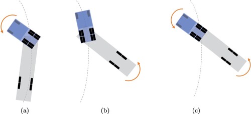
Without timely intervention (such as decreasing the applied brake or propulsion torques at the wheels, applying a counteracting yaw moment by differential braking, or steering), the severity of jackknifing usually increases and the tractor rotates around the fifth wheel until the two units collide (the tractor cab hits the semitrailer body).
2.2. Trailer swing
Trailer swing in AHVs is defined as a loss of directional stability of the trailing unit but not of the towing unit. This leads to an excessive articulation angle since the real direction of the trailing unit deviates significantly from the reference direction (intended direction of travel). Trailer swing occurs when the trailing unit loses lateral tyre grip and starts sliding sideways. Loss of lateral tyre grip is typically caused by excessive combined tyre slip under braking or acceleration during a turn. Figure (b) illustrates typical AHV trailer swing.
Unlike jackknifing, if trailer swing occurs under trailer braking, its severity may decrease over time due to a decrease in speed. If the driver detects the trailer swing in time, it can be corrected by releasing the brake pedal. However, if the trailer swing is not corrected in time, the semitrailer may cross onto another lane and hit other vehicles. Trailer swing can also occur under trailer propulsion (for electrified trailers). Similarly, it can be avoided by removing the propulsion torque. If the trailer swing is not avoided in time, the trailing unit can swing considerable, ultimately causing the towing unit to lose lateral grip and then swing.
2.3. Combination spin-out
Apart from jackknifing (when the tractor loses directional stability) and trailer swing (when the semitrailer loses directional stability), there is a third yaw instability mode for two-unit combination vehicles. In this paper, it is termed ‘combination spin-out’.
Combination spin-out in AHVs is defined as simultaneous loss of directional stability in both units. Unlike jackknifing or trailer swing, there may be no excessive articulation angle as the directions of both units deviate significantly from the reference direction. Combination spin-out occurs when both towing and trailing units lose lateral tyre grip and start sliding sideways. Loss of lateral tyre grip is typically caused by excessive combined tyre slip under braking or acceleration during a turn. Figure (c) illustrates typical AHV combination spin-out.
3. Modelling and simulations
This section introduces a nonlinear single-track model and then goes on to explain the simulated manoeuvres. Single-track model is a computationally efficient model that can be used to simulate thousands of different manoeuvres to evaluate the yaw stability. Furthermore, the single-track model can be used for eigenvalue stability analysis to explain the fundamental concepts of brake and propulsion forces allocation in AHVs.
3.1. Nonlinear single-track model
A nonlinear single-track model of the AHV (Equations (Equation1(1)
(1) )–(Equation9
(9)
(9) ), taken from [Citation23,p.296]) can be derived by considering the free-body diagrams shown in Figure [Citation23,p.296]. The tractor rear axle group and semitrailer axle group are modelled as single lumped axles. The nomenclature used in this paper is provided in Appendix 2.
Figure 2. Free-body diagrams of the nonlinear single-track model for the AHV [Citation23,p.296]. Forces and moments are shown in blue, velocities in green.
![Figure 2. Free-body diagrams of the nonlinear single-track model for the AHV [Citation23,p.296]. Forces and moments are shown in blue, velocities in green.](/cms/asset/bb0ac6cd-62a8-4ce7-8036-9dfef59a46e8/nvsd_a_2276767_f0002_oc.jpg)
The force equilibrium along the longitudinal and lateral axes and yaw moment equilibrium around the centre of gravity of the tractor are given by:
(1)
(1) The force equilibrium along the longitudinal and lateral axes and yaw moment equilibrium around the centre of gravity of the semitrailer are expressed as:
(2)
(2) The force equilibrium for the coupling between the tractor and semitrailer is obtained by the following equations:
(3)
(3) The compatibility equations for the velocities depicted in Figure for the tractor are obtained as follows:
(4)
(4) The compatibility equations for the semitrailer are given by:
(5)
(5) and the longitudinal and lateral velocities for the coupling are as follows:
(6)
(6) The rate of change in the articulation angle between the tractor and semitrailer is given by:
(7)
(7) The lateral wheel slips for the tractor and semitrailer are calculated as follows:
(8)
(8) In the lateral direction, a simple tyre model is used in which the lateral force is proportional to the wheel slips. The lateral tyre force on the tractor's front and rear axles and lumped axle of the semitrailer are then defined as follows:
(9)
(9) The single-track model used in this study combines the effects of all tyres on one axle into a single, virtual tyre. This model is nonlinear because of sine and cosine terms in Equations (Equation1
(1)
(1) ), (Equation3
(3)
(3) ), (Equation4
(4)
(4) ), (Equation6
(6)
(6) ), multiplication terms in Equations (Equation1
(1)
(1) ), (2), and division terms in Equation (Equation8
(8)
(8) ).
Based on this model, the tyres can generate an infinite amount of lateral force. This is not realistic for modelling jackknifing or trailer swing as these AHV modes usually occur when the wheels are experiencing major slips. Hence, a more advanced tyre model should be introduced to study jackknifing and trailer swing. The simplest addition involves adding saturation to the lateral forces, considering a friction circle model [Citation23,p.133]. To this end, the longitudinal tyre force inputs [,
,
] should be defined as follows:
(10)
(10) where μ is the tyre-road friction coefficient,
and
are the normal loads on the tractor's rear axle and semitrailer's lumped axle, respectively.
and
are the friction utilisation coefficients of the tractor and semitrailer, respectively. These coefficients vary within an interval of
for braking scenarios and
for propulsion scenarios. Thus, the values
and
correspond to the maximum braking and maximum propulsion, respectively.
For this study, the front axle of the tractor is considered to be a non-braked and non-powered axle. Thus, only the regenerative braking and electric propulsion of the tractor's rear axle and semitrailer axle are studied. The interaction between the combined longitudinal and lateral forces is often modelled using the well-known friction circle [Citation23,p.133]. For a vehicle undergoing braking or acceleration, the lateral forces are limited by the upper bound friction circle conditions provided by:
(11)
(11) Thus, the lateral forces defined as a function of the lateral wheel slips as in (Equation9
(9)
(9) ) are also saturated by the upper-bound friction circle condition introduced in (Equation11
(11)
(11) ) as follows:
(12)
(12) Finally, the equations given in (Equation9
(9)
(9) ) may be replaced by the equations introduced in (Equation12
(12)
(12) ). The steering angle
is considered to be a constant value throughout this study and is calculated according to the Ackermann steering geometry given by:
(13)
(13) The nonlinear single-track model (Equations (Equation1
(1)
(1) )–(Equation8
(8)
(8) ), (Equation11
(11)
(11) ) and (Equation12
(12)
(12) )) consisting of 27 equations can be solved for 27 unknowns, [
,
,
,
,
,
, θ,
,
,
,
,
,
,
,
,
,
,
,
,
,
,
,
,
,
,
,
] by using four known inputs, [
,
,
,
], given in Equations (Equation10
(10)
(10) ) and (Equation13
(13)
(13) ). All these equations can be written in a Modelica tool [Citation24], which can solve the set of implicit equations in a computationally efficient way: The system of 27 equations is converted to a linear dynamical system (ordinary differential equations) with 5 states and 22 (linear and nonlinear) algebraic equations. The 22 algebraic equations are solved successively by using the previously solved variables thanks to the block lower triangle partitioning. Additionally, the linear dynamical system is solved by using the previously solved variables. The numeric values of the parameters are given in Appendix 1.
The articulation angle is the most obvious state to check while studying such yaw instabilities as jackknifing and trailer swing. However, if both the vehicle units are sliding sideways at the same time (combination spin-out, as explained in Section 2.3), then checking the side-slip angles for the tractor's rear axle and semitrailer axle becomes more relevant since the side-slips of both units can be identified separately. The side-slip angles of the tractor's rear axle and semitrailer axle are calculated as follows:
(14)
(14) Furthermore, a normalised lateral acceleration
can be defined as follows:
(15)
(15)
3.2. Manoeuvre description
Braking-in-turn and propelling-in-turn manoeuvres are simulated, to investigate the stability of the AHVs and obtain an SOE. For all simulations conducted in this study, the steps followed are:
Unless otherwise stated, the vehicle starts to operate on a road with a friction coefficient of 0.3 (
).
Unless otherwise stated, the initial longitudinal velocity of the tractor is set to
The road wheel angle on the tractor's first axle is set according to Equation (Equation13
For the first 5 s, no longitudinal force is applied on the wheels. This is to let the AHV reach a quasi-steady-state. In other words,
At
For both braking and propulsion scenarios, the simulation is terminated if the articulation angle reaches
reaching zero velocity when braking is applied, as shown in the example manoeuvre given in Figure (b).
2 s after the application of propulsion. The reason for only 2 s of propulsion is that, as the longitudinal velocity increases due to the propulsion, the lateral acceleration also increases. Hence jackknifing or trailer swing eventually occurs when all the lateral forces are saturated. The intent is to study ‘instantaneous’ dynamics, corresponding to the lateral acceleration when the propulsion started. Furthermore, in the real (brake-in-turn) tests, the authors have observed that a yaw instability usually takes place within the first 2 s of application of tyre forces. In this specific context, the selected time interval until termination of the simulations (2 s) is called the ‘time horizon’ (not to be confused with the time horizon of a predictive control).
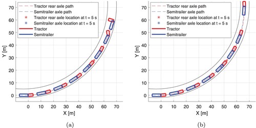
Figure 3. Paths followed by an AHV for two different braking manoeuvres with km/h,
, R = 72 m. Braking starts at
. (a)
and
. Jackknifing occurs and simulation is terminated when the articulation angle reaches
and (b)
and
. No yaw instability occurs and simulation is terminated when the tractor reaches zero velocity.
4. Stability analysis of AHVs
In this section, first, a stability analysis of the linearised AHV model is conducted by evaluating the eigenvalues. This is then followed by investigating the effect of different parameters on the yaw stability of the AHV model. Finally, safety criteria for classifying a manoeuvre as stable are introduced.
4.1. Eigenvalue stability analysis
To perform a stability analysis using the model's eigenvalues, it is necessary to linearise the model first. To do this, the AHV is simulated according to the first five steps explained in Section 3.2. The simulation is then stopped at (100 ms after applying propulsion or braking forces). The nonlinear system equations (Equations (Equation1
(1)
(1) )–(Equation8
(8)
(8) ) and (Equation10
(10)
(10) )–(Equation13
(13)
(13) )) are then linearised around the states at
.
The real and imaginary parts of the system's eigenvalues corresponding to five different pairs of are illustrated in Figure . Furthermore, the eigenvalues of the actuated model are also provided in Table for 13 different sets of
.
Figure 4. Eigenvalues of the linearised single-track model, actuated with five different longitudinal force pairs. is the friction utilisation of the tractor's rear axle and
is the friction utilisation of the semitrailer's axle.
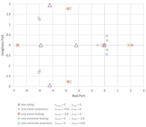
Table 1. Eigenvalues of the nonlinear single-track model actuated with 13 different longitudinal force pairs.
Within the first 5 s of the simulations, for the initial condition of km/h and
, the lateral acceleration of the tractor reaches
. As the friction coefficient, μ is set to 0.3 (corresponding to the friction coefficient on snow), the maximum lateral acceleration the AHV can reach is
.
As shown in Figure and Table , for the case in which (when all the longitudinal forces are zero), all the eigenvalues have negative real parts. This implies that the AHV model with no longitudinal actuation is stable.
Modern anti-lock braking systems usually try to keep the longitudinal forces less than the maximum capability (within the linear region of the slip vs tyre force curve, as explained in [Citation25]). This is done to leave some of the tyre force capability for the lateral grip. Hence, as an example to study, the friction utilisation value of 0.8 is considered and results in four different cases: ,
,
,
. The eigenvalues of the model for these cases are illustrated in Figure and Table .
Braking or propelling the tractor and/or semitrailer (singly or together) with high friction utilisation ratios and
, results in the real parts of the eigenvalues being shifted towards the positive half-plane, implying instability. According to Table , braking with
and propelling with
also makes the AHV unstable. On the other hand, the eigenvalues for the lower (in the absolute sense) values of the friction utilisations, such as
, have negative real parts. This implies stability.
4.2. Safety assessment criteria for stability
The following criteria are used to define a manoeuvre as safe in terms of yaw stability:
(16)
(16)
The selected limit of is sufficiently high, at
. This is done to avoid covering the deviations that occur even during normal (safe) driving. Typically, these can be of the order of several degrees. However, the limit of
, is deliberately maintained at a lower value. Semitrailers are longer than tractors. Thus, a side-slip angle of
at the semitrailer (at approximately
from the kingpin to the rear of the semitrailer), will create a lateral displacement of
at the rear end of the semitrailer. This will likely cause the semitrailer to leave its lane.
The maximum deviation of the articulation angle is not used as a safety criterion in Equation (Equation16(16)
(16) ). This is because the articulation angle alone is not a sufficient measure for identifying yaw instability. As explained in Section 2.3, the articulation angle does not necessarily grow during a combination spin-out, even though the side-slip angles of the units grow. Even though not used in this study, the articulation angle may be used as a complementary criterion to the side-slip angle deviation limits given in Equation (Equation16
(16)
(16) ). Nevertheless, articulation angle is an important state to evaluate apart from the side-slip angles, and it is given in some plots of this study.
4.3. Stability analysis in the time domain
This section discusses the effects of different vehicle and environmental parameters on yaw stability. To this end, the AHV is simulated for different cases according to the methodology explained in Section 3.2. The AHV is braked only on the trailer axle at , with the friction utilisation
. After the braking forces are applied, the AHV becomes unstable.
and θ grow in the negative direction while
grows in the positive direction, as shown in Figure . Meanwhile,
reaches saturation level
for 2.7 s. As the lateral acceleration decreases due to the braking and longitudinal speed reduction,
drops below the limit, with
, θ, and
consecutively returning to quasi-steady-state values. Hence, after the decrease in the longitudinal speed and lateral acceleration, the unstable system becomes stable again for the given amount of braking force. This means the instability only lasts 2.7 s and then the system stabilises itself.
The maximum deviations of the articulation and side-slip angles (from the quasi-steady-state values) are three ideal performance metrics for evaluating the yaw instabilities of AHVs. The quasi-steady-state values of ,
and θ are obtained at
for the given operating conditions, as the braking/propulsion starts at
, as explained in Section 3.2. Thanks to these three performance measures, it is possible to evaluate a single manoeuvre using only three values, instead of checking signals as a function of time. This simplifies parametric studies.
Figure 5. AHV exhibiting a trailer swing due to semitrailer braking, with at
.
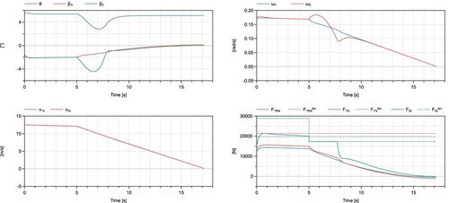
Figure depicts ,
and
, which are the maximum deviations (over time) for
,
and θ from their quasi-steady-state values throughout each simulation for various turning radii, initial longitudinal speeds and friction coefficients. As shown in Figure (a), when only the tractor brakes with
, jackknifing occurs at around
regardless of changes in the path radius, initial speed or friction coefficient. Any parameter change that creates a greater normalised lateral acceleration of more than
leads to jackknifing. This is slightly more than expected, since
, and
already mean that the rear tyre forces at the tractor are approaching the friction circle limit, according to Equation (Equation11
(11)
(11) ). However, this difference can be explained by the fact that the AHV is slowing down and the lateral tyre forces are saturated for only a limited time for
. But for
, the AHV undergoes saturated lateral tyre forces at the rear axle of the tractor for long enough for jackknifing to occur. Another observation is that either severe jackknifing occurs,
, with
reaching approximately
(and leading to a terminated simulation), or no jackknifing occurs at all. So, unlike trailer swing, the magnitude of jackknifing does not progressively increase with greater lateral acceleration. Once jackknifing starts, θ and
grow rapidly and do not decrease with time when the longitudinal velocity and lateral acceleration decrease.
does not grow under the same manoeuvres and thus, jackknifing does not cause the semitrailer to swing.
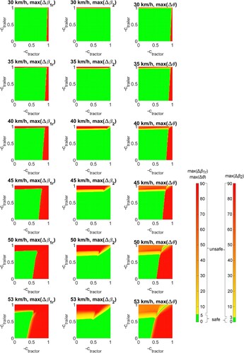
Figure 6. Changes in maximum articulation angle and side-slip angle deviations due to different values on the operational parameters: turning radius (first-row plots), initial speed (second-row plots), and friction coefficient (third-row plots) for three different braking manoeuvres. (a) (b)
(c)
![Figure 6. Changes in maximum articulation angle and side-slip angle deviations due to different values on the operational parameters: turning radius (first-row plots), initial speed (second-row plots), and friction coefficient (third-row plots) for three different braking manoeuvres. (a) [ctractorctrailer=−0.80] (b) [ctractorctrailer=0−0.8] (c) [ctractorctrailer=−0.8−0.8]](/cms/asset/eda407a9-273f-443b-a80a-f8451867fc2c/nvsd_a_2276767_f0006_oc.jpg)
According to Figure (b), when braking only with a semitrailer at , trailer swing (with max(
) starts at around
regardless of path radius, initial speed or friction coefficient. Any parameter change that creates greater normalised lateral acceleration (over
) leads to trailer swing. However, the trailer swing becomes stronger (greater semitrailer side-slip angle and articulation angle deviation) as the lateral acceleration increases. This is not like jackknifing, so the severity of the trailer swing increases progressively under greater lateral acceleration. Trailer swing starts at higher lateral acceleration values compared to the previous scenario. Lateral acceleration then drops, due to the speed reduction after braking. Hence
and θ stabilise again around the quasi-steady-state values. As the tractor has no longitudinal force in this manoeuvre, it is stable until very large
values. For greater initial speeds and lower friction coefficients resulting in
values close to 1,
also grows very quickly and the tractor loses its lateral grip due to the saturated lateral tyre forces, according to the first and the second equations in (Equation11
(11)
(11) ).
Finally, as shown in Figure (c), when both the tractor and semitrailer brake with and
, the tractor loses its lateral grip and quickly reaches a
side-slip angle at around
. This is a greater value compared to the first scenario, in which only the tractor was braked. This is because the greater retardation caused by braking on both vehicle units leads to a faster reduction in lateral acceleration compared to the first case. However,
increases progressively for the greater lateral acceleration but the increase is not stepwise as with the tractor.
Jackknifing starts (in the first manoeuvre) at , and trailer swing starts (in the second manoeuvre) at
. This shows that braking the tractor is more unstable than braking the semitrailer. This phenomenon can be explained by studying the real parts of the eigenvalues in the corresponding manoeuvres, as shown in Figure and Table . When only the tractor is braked (with
), the real part of the positive eigenvalues is much greater compared to the case when only the semitrailer is braked (with
). Hence, braking on the tractor is even less stable than braking on the semitrailer. Furthermore, braking the tractor is also less stable than propelling it, as the real part of the largest positive eigenvalue is greater. This is physically determined by a compression force at the coupling (due to the tractor braking) making the AHV less stable; the tractor is pushed adversely by the semitrailer. Conversely, semitrailer braking results in a tension force at the coupling and pulls the tractor backwards, creating a ‘stabilising yaw moment’ for it.
Figure illustrates the effects of variations in and
on
,
and
. This analysis was made by keeping the friction utilisation for one vehicle unit at zero (no longitudinal force applied), while the other one varied within the considered range of
. For positive friction utilisation ratios (propulsion case), limiting the simulation to only 2 s of propulsion led to a gradual increase in the tractor side-slip angle and articulation angle deviation values. This contrasts with the stepwise increases in the negative friction utilisation ratios (braking case).
Figure 7. Effects of various friction utilisation ratios, and
. (a)
and
and (b)
and
.
![Figure 7. Effects of various friction utilisation ratios, ctractor and ctrailer. (a) ctractor∈[−1,1] and ctrailer=0 and (b) ctractor=0 and ctrailer∈[−1,1].](/cms/asset/c41e1d5f-3bed-42c6-bb69-8523411e925a/nvsd_a_2276767_f0007_oc.jpg)
As can be seen in Figure (a), jackknifing (with max() occurs while braking with
or less; or with propulsion of
or more. This shows that propelling the tractor is more stable than braking it, which can also be explained using the eigenvalues shown in Figure . As shown in Figure (b), the trailer swing occurs (with max(
) under braking with
or less. And for propulsion it occurs for
or more. This shows that propelling the semitrailer causes more instability than braking it. Furthermore, these pairs of
and
for braking and propulsion cases prove that braking on the semitrailer is more stable than braking on the tractor, and propelling on the tractor is more stable than propelling on the semitrailer. The common characteristic of more stable actuations, namely tractor propulsion and semitrailer braking, is that they increase the tension force at the coupling which has a stabilising effect.
5. Safe operating envelope for AHVs
The ‘safe operating envelope’ (SOE) is the term for a set of upper and lower request limits on the actuators. These include braking or propulsion force requests, expressed as a function of vehicle states (such as vehicle longitudinal speed and lateral acceleration), alongside environmental parameters (such as road friction, road slope and so on). Control algorithms whose design is based on an SOE keep the vehicle safe and allow it to manoeuvre up to its handling limits without risking yaw stability.
This section simulates the nonlinear single-track model of a tractor-semitrailer combination vehicle (as per Section 3.1), according to the methodology explained in Section 3.2 in Modelica. Based on many simulations involving different parameters, safe and unsafe scenarios have been identified for a vehicle negotiating turns. Consequently, an SOE is obtained. The vehicle parameters are provided in Appendix 1.
By varying the values of ,
, and
, many different combinations of longitudinal tyre forces for two vehicle units and different lateral tyre forces have been simulated. In other words, the simulations were conducted by changing
and
from
to 0 (in steps of −0.01) for the braking scenarios and from 0 to +1 (in steps of +0.01) for the acceleration scenarios using various values of
km/h. This requires 61,206 simulations to be conducted for each braking and propulsion scenario.
For the initial part of the manoeuvres, the quasi-steady-state lateral accelerations are noted for (half a second before applying braking or propulsion forces) as
. This set of lateral accelerations can be normalised with respect to the gravitational constant g and the friction coefficient μ, as
.
5.1. Safe operating envelope for braking
The values of ,
and
for different
,
and
values are shown in Figure . A colour map is used to indicate the safe and unsafe operating areas which are obtained based on
,
, and
. Equation (Equation16
(16)
(16) ) is used as a safety criterion. A limit of
is used for
, although it is not a part of Equation (Equation16
(16)
(16) ). Yellow and red are associated with lower and higher unsafe operating conditions, while green indicates safe operating conditions.
Figure 8. Maximum side-slip angle and articulation angle deviations for braking at six different speeds, according to the nonlinear single-track model.
In Figure , the red stripe at the top of each plot shows that, even at low lateral accelerations, values which are very close to
, resulting in trailer swing as the semitrailer wheels lose side grip. Hence,
grows. If it becomes too significant (when
becomes red in Figure ), then the aggressively swinging trailer causes the tractor to start losing side grip and also begin to swing. At higher lateral accelerations, the semitrailer also swings at lower
values (in the absolute sense);(
=-0.56 for a speed of 53 km/h). The red areas at the top of each plot are almost straight and do not change much in thickness with varying
values. This means that the trailer swing is not highly correlated with the amount of tractor braking. Nevertheless, greater tractor braking marginally helps to avoid trailer swing since it results in a faster reduction in speed and lateral acceleration.
In Figure , looking at the red diagonal areas on the right-hand side of the first and third column plots reveals that high (in the absolute sense) friction utilisation in the tractor ( values close to
) produces a major deviation in the tractor's side-slip angle but not in that of the semitrailer. This is a sign of jackknifing.
The risk of jackknifing is inversely proportional to the degree of semitrailer braking. For a high degree of semitrailer braking ( values close to
), the width of the red diagonal area decreases. This means that stretch braking with the semitrailer helps avoid jackknifing. Conversely, when there is no semitrailer braking, jackknifing starts at a lower degree of tractor braking.
The green areas at the upper right of the lower three plots (third column plots) in Figure show that, even though the side-slip angles of the tractor and semitrailer increase, the articulation angles for those specific manoeuvres are still small. This is a sign of combination spin-out. In other words, the tractor and semitrailer simultaneously lose their side grip, slipping sideways in a rigid-body motion, as explained in Section 2.3.
A final observation from Figure is that the green areas reduce as the lateral acceleration increases. This is expected since greater lateral acceleration leads to greater lateral forces at the tyres and the friction circle model will lead to the tyre forces being saturated with lower braking forces (longitudinal forces).
Figure (a) shows the SOEs for six different longitudinal velocities (six different lateral accelerations). These envelopes show safe combinations of tractor and semitrailer friction utilisation factors ( and
) as green, with unsafe combinations in red. The safe combinations are calculated according to the safety criteria given in Equation (Equation16
(16)
(16) ).
Figure 9. SOE obtained from the nonlinear single-track model of a braking AHV.
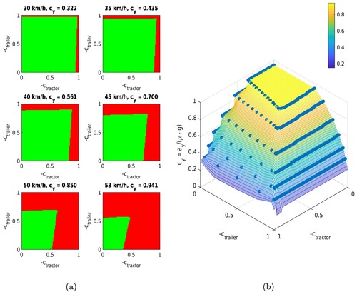
Figure (b) shows a three-dimensional SOE obtained by using the previous six plots and interpolating the intermediate values. So, the six plots on the left are slices of the three-dimensional plot on the right. The vertical axis on the three-dimensional envelope plot represents normalised lateral acceleration (with respect to μ and g), , as calculated in Equation (Equation15
(15)
(15) ).
Any combination of tractor and semitrailer braking ( and
) under the safe operating envelope shown in Figure (b) is a safe braking manoeuvre and, according to the nonlinear single-track model, causes no motion instability. However, any braking combination above the safe operating envelope violates the safety criteria given in Equation (Equation16
(16)
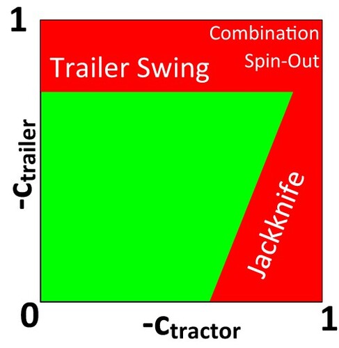
(16) ) and causes jackknifing, trailer swing or combination spin-out. These three modes of instability are shown in a generic SOE plot in Figure . A large (in the absolute sense)
results in trailer swing, while large (in the absolute sense)
results in jackknifing. Combinations of large
and
result in combination spin-out.
Figure 10. Different yaw instability modes shown on the SOE.
5.2. Safe operating envelope for acceleration
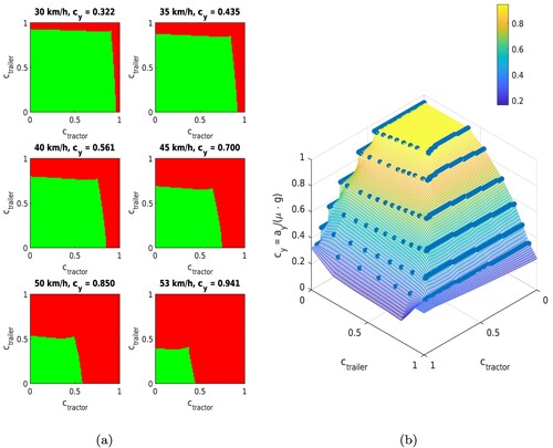
Figure shows an SOE for an accelerating AHV, obtained from the nonlinear single-track model presented in Section 3.1. Note that the normalised lateral acceleration values for each plot indicate the values to be 0.5 s before the specified propulsion force is applied. However, unlike the braking case, as the speed increases following application of propulsion torque, the normalised lateral acceleration
values grow even more.
Figure 11. SOE obtained from the nonlinear single-track model of an accelerating AHV.
In the case of a longer time horizon to terminate the simulation (and hence ceasing to evaluate the presence of yaw instability according to Equation (Equation16(16)
(16) )), the unsafe red areas would be greater because the normalised lateral acceleration would also be greater, leaving less tyre force capability for the longitudinal direction. Hence, the safe operating envelope would contract. Similarly, in the case of a shorter time horizon to terminate the simulation, the safe operating envelope would expand.
By comparing Figures and , it may be observed that the trailer swing areas (red area at the top of each subplot corresponding to high coefficients) are greater in the case of acceleration. This is because the trailer propulsion is more unstable compared to trailer braking, as explained in Section 4.3. However, the border of the trailer swing area (red area at the top of each subplot) is still almost parallel to the x-axis, showing that trailer swing occurs above a certain
coefficient, almost independent of the
value. This means that trailer swing does not highly correlate to the degree of tractor propulsion (and braking, as shown in Section 5.1).
By comparing Figures and , it may also be observed that the border of the jackknifing area (the red area on the right-hand side of each subplot) is inclined in the opposite direction. In the case of acceleration, a greater (in the absolute sense) is safe and stable (green) for a lower (in the absolute sense)
. This is the opposite situation to that of braking and means that, by applying a lower propulsion force at the semi-trailer (lower
), a greater propulsion force may be applied at the tractor (greater
) without causing a yaw instability. Furthermore, a comparison of Figures and shows that yaw instabilities start at a greater (in the absolute sense)
for tractor propulsion, compared to tractor braking (while the semi-trailer is neither braked nor propelled,
, for the sake of comparison). This shows that tractor propulsion is more stable compared to tractor braking, as shown in Section 4.3.
Figure shows a slice of the SOE obtained from the nonlinear single-track model for the velocity of 40 km/h (). In this figure, the axes associated with
and
are plotted between
and 1, implying that this plot covers any combination of braking and propulsion. So, the first quadrant of this plot is already shown in Figure and the third quadrant is already shown in Figure . The second and fourth quadrants are not presented in any other plot and are combinations of tractor braking and semitrailer propulsion and tractor propulsion and semitrailer braking, respectively. The last two cases are not energy-efficient and would be mostly irrelevant during normal driving. But for any safety-related function, they may still be related and these SOEs can be used for such cases. Furthermore, these areas may be used to transfer energy stored in the batteries from one unit to another (regenerative braking in one unit and propulsion with the other). Regarding the maximum and minimum braking and propulsion forces and the correlation of tractor and semi-trailer forces, all the above comments are valid for Figure too. It is also possible to obtain a complete three-dimensional SOE by combining many such slices for different normalised lateral accelerations (
), as presented in Figures and .
Figure 12. Slice of the SOE obtained from the nonlinear single-track model for 40 km/h () for any combination of propulsion and braking forces.

6. Conclusion
This paper has described the yaw instabilities of AHVs and presented a nonlinear single-track vehicle model for an AHV. The factors affecting yaw instabilities have also been investigated. Lastly, safe operating envelopes for both braking and accelerating AHVs have been obtained.
A nonlinear single-track vehicle model is a computationally effective way to derive an SOE. The SOE can be determined every second (or at any another suitable time interval) online at the AHV's electronic control unit for instantaneous operating conditions. Hence, this SOE can adapt to changes in the vehicle parameters (such as load distribution) or environmental changes (such as slope and friction). Furthermore, the single-track model may be used to predict the AHV's states at a given future time (1 s later, for example) with a driver model. Moreover, if instability is predicted, then precautionary action may be taken (such as decreasing the propulsion or braking forces, or redistributing them).
The SOE can be used with simple rule-based control allocation methods for actuator coordination. Ideally, however, it can be also used with closed-loop controllers (such as the one described in [Citation22]). In this case, the SOE would act as the first-level safety measure. Should the SOE fail to ensure safety, the second level would be the closed-loop controller.
The single-track model is not accurate for high lateral accelerations (since the lateral load transfer has not been modelled). Hence, the SOE for the high lateral accelerations is expected to be both less accurate and greater than the real safe operating conditions. The SOE obtained from the single-track model may be shrunk by a safety factor (such as 50% less than the SOE obtained from the simulations) for use in real applications. Shrinking the SOE by a (lower) safety factor (say, 25%) may also be done for lower lateral accelerations, to handle the parameter and model uncertainties. Furthermore, a two-track model [Citation23,p.306] may be used to take the lateral load transfer into account.
The presented single-track model has lumped axles for axle groups. To make the model more accurate, all the axles can be modelled individually. This would increase the model's complexity but it would still be computationally efficient compared to the high fidelity models.
The tyre model used in the simulations is a linear type with saturation according to the friction circle model. This is a simple yet efficient model but can be replaced with a more advanced one, such as the Pacejka tyre model [Citation26].
No slip controller was used for the simulations. But in a real AHV, even though or
are requested, the realised friction utilisation would be no more than approximately 0.8 for the modern brake and traction control systems (which corresponds to the linear region of the slip vs tyre force curve, as explained in [Citation25], for example). Hence, the unsafe (red) areas of 30 km/h and 35 km/h plotted in Figures and would not be reached in a real AHV thanks to the slip controller in the brake or traction control system, provided these systems perform well. Nevertheless, a simple slip controller may be added to the simulations to take this into account.
For all simulations, the steering angle was kept constant after the application of propulsion or brake torque. Hence, a human driver or autonomous system is not trying to stabilise the AHV. In reality, a human driver or autonomous safety system would try to stabilise it, meaning that the limiting unsafe cases may become safe within the closed-loop of a human or autonomous system. From this point of view, the SOE obtained takes the worst-case scenario (an uncontrolled vehicle) into account.
In the other studies in the automotive field which focus on the safe operating envelope, side-slip angles and yaw rates are mostly the states used to define the SOE for a single-unit vehicle [Citation16–20]. Hansson et al. [Citation21], on the other hand, focus on actuator coordination of AHVs. However, this has an SOE obtained via offline high-fidelity simulations and is only defined for semitrailer propulsion. Furthermore, the states (velocity, friction coefficient, coupling forces in longitudinal and lateral directions, propulsion torque applied at the semitrailer) used to define the SOE are different. However, in the present study, the SOE is defined in terms of actuator force (normalised with normal load and friction) allocation per unit (for both tractor and semitrailer) for an AHV, for both braking and propulsion cases. Defining SOE in terms of actuator forces (instead of, for example, coupling forces, and so on) makes it easier to envision how the control inputs should be limited for safe driving since the control inputs are the actuator forces per unit. Furthermore, it also makes it easier to implement the SOE in a controller; the SOE becomes constraints on the inputs, instead of some states that are to be estimated via a model or measured with sensors. Nevertheless, the SOE is also a function of lateral acceleration (normalised with friction). Furthermore, the SOE is obtained with a simpler and computationally more efficient single-track model that can be run online.
In future work, the SOE obtained from the nonlinear single-track model should be verified with real tests. As it is not possible to cover all possible cases within real tests, a high-fidelity model (validated with respect to the real test vehicle) should be used to cover all possible cases. The single-track model presented here should be improved according to the alternatives explained above and checked to see that it is safe enough for a real application. The improved model may be used to obtain SOE online for the real AHVs as the first safety level of the safe and energy-efficient actuator coordination controllers. The nonlinear single-track model provides valuable insight into instability onset, but moving forward, a more refined model can be used to deliver more quantitative results and reliable instability predictions.
Disclosure statement
No potential conflict of interest was reported by the author(s).
Correction Statement
This article has been corrected with minor changes. These changes do not impact the academic content of the article.
Additional information
Funding
References
- Bienkowski BN, Walton CM. The economic efficiency of allowing longer combination vehicles in Texas. Center for Transportation Research, The University of Texas at Austin; 2011. (Research report, SWUTC/11/476660-00077-1). Available from: https://rosap.ntl.bts.gov/view/dot/23703.
- Backman H, Nordström R. Improved performance of European long haulage transport. TFK – Institutet för transportforskning; 2002. (TFK report). Available from: https://books.google.se/books?id=5YQMkAEACAAJ.
- Woodrooffe J, Ash L. Economic efficiency of long combination transport vehicles in Alberta. Woodrooffe & Associates; 2001. Available from: https://open.alberta.ca/publications/final-report-economic-efficiency-of-long-combination-transport-vehicles-in-alberta.
- Dunn AL. Jackknife stability of articulated tractor semitrailer vehicles with high-output brakes and jackknife detection on low coefficient surfaces [dissertation]. Columbus (OH): The Ohio State University; 2003. Available from: http://rave.ohiolink.edu/etdc/view?acc_num=osu1061328963.
- Bouteldja M, Koita A, Dolcemascolo V, et al. Prediction and detection of jackknifing problems for tractor semi-trailer. In: Proceedings of the 2006 IEEE Vehicle Power and Propulsion Conference; 2006 Sep 6–8; Windsor, United Kingdom: IEEE; 2006. Available from: https://ieeexplore.ieee.org/document/4211300.
- Bouteldja M, Cerezo V. Jackknifing warning for articulated vehicles based on a detection and prediction system. In: Proceedings of the 3rd International Conference on Road Safety and Simulation; 2011 Sep 14–16; Indianapolis (IN). Available from: https://onlinepubs.trb.org/onlinepubs/conferences/2011/RSS/3/Bouteldja,M.pdf.
- Kaneko T, Kageyama I, Tsunashima H. Braking stability of articulated vehicles on highway. Veh. Syst. Dyn. 2002;37(sup1):1–11. doi: 10.1080/00423114.2002.11666216
- VLK F. Lateral dynamics of commercial vehicle combinations a literature survey. Veh. Syst. Dyn.1982;11(5–6):305–324. doi: 10.1080/00423118208968702.
- Federal Motor Carrier Safety Administration Analysis Division. Large truck and bus crash facts 2017. U.S. Department of Transportation; 2019. Available from: https://www.fmcsa.dot.gov/sites/fmcsa.dot.gov/files/docs/safety/data-and-statistics/461861/ltcbf-2017-final-5-6-2019.pdf.
- van Oort ER, Chu QP, Mulder JA. Maneuver envelope determination through reachability analysis. In: Holzapfel F, Theil S, editors. Advances in Aerospace Guidance, Navigation and Control: Selected Papers of the 1st CEAS Specialist Conference on Guidance, Navigation and Control; 2011 Apr 13–15; Munich, Germany: Springer; 2011. p. 91–102. doi: 10.1007/978-3-642-19817-5.pdf
- Lombaerts T, Schuet S, Acosta D, et al. On-line safe flight envelope determination for impaired aircraft. In: Bordeneuve-Guibé J, Drouin A, Roos C, editors. Advances in Aerospace Guidance, Navigation and Control: Selected Papers of the Third CEAS Specialist Conference on Guidance, Navigation and Control; 2015 Apr 13–15; Toulouse, France: Springer; 2015. p. 263–282. doi: 10.1007/978-3-319-17518-8.pdf
- Lombaerts T, Schuet S, Wheeler K, et al. Safe maneuvering envelope estimation based on a physical approach. In: Proceedings of the AIAA Guidance, Navigation, and Control (GNC) Conference; 2013 Aug 19–22; Boston (MA): AIAA; 2013. doi: 10.2514/6.2013-4618
- Zhang Y, De Visser C, Chu QP. Online safe flight envelope prediction for damaged aircraft: a database-driven approach. In: Proceedings of the AIAA Modeling and Simulation Technologies Conference; 2016 Aug 19–22; Boston (MA): AIAA; 2016. Available from: https://pure.tudelft.nl/ws/portalfiles/portal/10445072/Ye_postprint_2.pdf.
- Park JY, Kim N. Design of a safety operational envelope protection system for a submarine. Ocean Eng. 2018;148:602–611. doi: 10.1016/j.oceaneng.2017.11.016
- Prime R, McIntyre M, Reeves D. Implementation of an improved safe operating envelope. In: Proceedings of the International Youth Nuclear Congress; 2008 Sep 20–26; Interlaken, Switzerland: IYNC; 2008. p. 408.1–408.7. Available from: https://inis.iaea.org/collection/NCLCollectionStore/_Public/40/048/40048172.pdf.
- Brown M, Funke J, Erlien S, et al. Safe driving envelopes for path tracking in autonomous vehicles. Control Eng. Pract. 2017;61:307–316. doi: 10.1016/j.conengprac.2016.04.013
- Cui Q, Ding R, Wei C, et al. Path-tracking and lateral stabilisation for autonomous vehicles by using the steering angle envelope. Veh. Syst. Dyn. 2021;59(11):1672–1696. doi: 10.1080/00423114.2020.1776344
- Bobier CG, Gerdes JC. Staying within the nullcline boundary for vehicle envelope control using a sliding surface. Veh. Syst. Dyn. 2013;51(2):199–217. doi: 10.1080/00423114.2012.720377
- Bobier CG, Gerdes JC. Envelope control: stabilizing within the limits of handling using a sliding surface. In: IFAC Proceedings Volumes. 6th IFAC Symposium on Advances in Automotive Control; 2010 Jul 12–14; Munich, Germany, vol. 43(7). IFAC; 2010. p. 162–167. Available from: https://www.sciencedirect.com/science/article/pii/S1474667015368233.
- Beal C, Bobier C, Gerdes J. Controlling vehicle instability through stable handling envelopes. In: Proceedings of the ASME 2011 Dynamic Systems and Control Conference and Bath/ASME Symposium on Fluid Power and Motion Control; 2011 Oct 31–Nov 2; Arlington (VA): ASME; 2011.
- Hansson A, Andersson E, Laine L, et al. Control envelope for limiting actuation of electric trailer in tractor-semitrailer combination. In: Proceedings of the 2022 IEEE 25th International Conference on Intelligent Transportation Systems (ITSC); 2022 Oct 8–12; Macau, China: IEEE; 2022. p. 3886–93.
- Tagesson K, Sundstrom P, Laine L, et al. Real-time performance of control allocation for actuator coordination in heavy vehicles. In: Proceedings of the 2009 IEEE Intelligent Vehicles Symposium; 2009 Jun 3–5; Xi'an, China: IEEE; 2009. p. 685–690.
- Jacobson BJH. Vehicle dynamics compendium. Gothenburg (Sweden): Chalmers University of Technology; 2020.
- modelica.org [Internet]. Munich (Germany): The Modelica Association; [cited 2022 Sep 20]. Available from: https://modelica.org/.
- Arikere A, Fröjd N, Henderson L, et al. Volvo Truck Corporation, assignee. Inverse tyre model for advanced vehicle motion management. United States patent US 2022/0126799 A1. 2022 Apr 28. Available from: https://patentimages.storage.googleapis.com/11/35/96/d8c96063aaf19e/US20220126799 A1.pdf.
- Pacejka HB. Tyre and vehicle dynamics. 2nd ed. Oxford (UK): Butterworth-Heinemann; 2005.
Appendices
Appendix 1.
Vehicle parameters
Table
Appendix 2.
Nomenclature
Table