Dynamic vehicle–track interaction and loading in a railway crossing panel – calibration of a structural track model to comprehensive field measurements

Abstract

This paper presents a finite element model of a railway crossing panel for use in multibody simulations (MBS). It is a two-layer track model with rails and sleepers represented by beam elements that use linear bushings for rail fastenings and non-linear bushings for ballast. The model is calibrated and validated to measurement data from a comprehensively instrumented switch and crossing demonstrator installed in the Austrian railway network as a part of the European research programme Shift2Rail. The validation concerns the capability of the model to capture the structural response of the crossing panel under traffic loading after calibration of physical track parameters to realistic values. The structural response is measured in the form of displacements, strains, and sleeper-ballast contact forces. It is shown that the developed model can represent the measured track responses well and that it was necessary to account for a varying sleeper-ballast gap distribution along the crossing transition sleeper to obtain good agreement. The calibration uses Latin hypercube samples to explore the parameter space in a sensitivity analysis before a parameter optimisation is performed using a gradient-based method on a response surface built from a polyharmonic spline.

KEYWORDS:

• Switches and crossings
• turnout
• measurements
• dynamic vehicle–track interaction
• calibration
• response surface

Introduction

A so-called Whole System Model (WSM) for railway switches and crossings (S&Cs, turnouts) is developed within the European research programme Shift2Rail and its In2Track projects [1]. The objective is that this model should allow for a holistic simulation-based assessment of S&C designs. In the WSM, dynamic interaction between S&C and passing vehicles is considered along with the loading and deterioration of S&C components over time. An iterative approach is applied where damage increments are computed and accumulated in the model for increments of traffic loading. Given the vast differences in length and time scales involved in dynamic vehicle–track interaction compared to long-term track degradation, it is not feasible for a single model to capture all relevant aspects of long-term S&C deterioration and performance. The WSM is therefore a framework that integrates state-of-the-art simulation tools and techniques.

While the literature contains several demonstrations of iterative schemes that compute accumulated damage in S&C for switch panels [2], crossing panels [3,4] and ballast [5], the WSM considers simultaneous deterioration in multiple damage modes allowing for the study of interaction between damage mechanisms [6]. This makes the WSM useful for the evaluation of different maintenance regimes in addition to design studies.

At the core of the WSM is a multibody simulation model for the evaluation of dynamic vehicle–S&C interaction that generates the responses needed for damage calculations. The first large-scale demonstration of the WSM scheme [6] used an MBS model with a co-running track model from the S&C benchmark [7]. In such models, the track structure is represented by a planar system of rigid bodies, springs and dampers that runs with each wheelset. While being computationally efficient [8], this means that the physical response of the track structure below the rails cannot be extracted without further postprocessing steps or approximations. The purpose of the developments presented in this paper is therefore to introduce a structural finite element track model into the MBS model. The model uses beam elements to represent rails and sleepers and bushing elements for rail fastenings and support stiffness. The model is implemented into the commercial multibody systems (MBS) software Simpack using substructure elements of the rail and sleeper bodies [9]. This type of modelling allows for the extraction of physical responses in the track structure in the form of nodal displacements. These can in turn be used to compute the structural loading in the form of loads in rails and sleepers due to bending, as well as sleeper-ballast contact pressures.

There are several previous efforts demonstrating structural track model representations of S&Cs using similar modelling approaches [10–14]. The main additions of the present model in terms of functionality are parameterised bi-linear stiffnesses to model a void distribution between sleeper and ballast, and a postprocessing step to extract bending moments and strains in rails and sleepers to quantify the structural loading. The model is also parameterised and script-generated to allow for easy generation of S&Cs of different sizes and properties.

Studies on the influence of voided (hanging) sleepers in S&C are not very common in the literature. Previous studies include Ref. [15] where a finite element model was used to investigate the effect of a completely voided sleeper. The influence of the stiffness variation along S&C was investigated in Ref. [16] and the influence of different assumed ballast stiffness distributions under a sleeper in the crossing panel was investigated in Ref. [17].

The developed model is calibrated to measurement data from a comprehensively instrumented S&C demonstrator. For a total of 23 sensors, the calibration evaluates the capability of the model to capture the structural response in the crossing panel under traffic loading in terms of rail and sleeper displacements and strains, as well as sleeper-ballast contact pressure. There are many studies that report analysis of measured track responses from crossing panels. Most of them have used a single accelerometer [18–21], while there are also examples with strain gauges [22], or both strain gauges and accelerometers [23]. Further, there are studies where geophones have been used to measure displacement along a longer distance of the S&C [16]. In Ref. [24], geophones, accelerometers and strain gauges were used to measure the structural response in a crossing panel under traffic loading. Out of the studies found, only Ref. [24] has a similar level of instrumentation detail as in the present study.

S&C design and installation

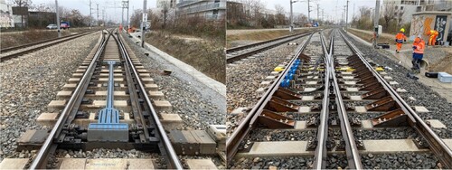
The studied S&C is a 60E1-500-1:12 demonstrator installed in the Austrian network as a part of the In2Track projects that are part of the EU-sponsored Shift2Rail research programme, see Figure 1. It is built from 60E1 rails and has a nominal radius of 500 m and a turnout angle of 1:12. The S&C is located between Vienna and Liesing and is situated in a track section with a radius of 3500 m. The demonstrator features novel developments compared to a standard design: it uses a soft rail fastening system, under sleeper pads, a new crossing rail design and a sleeper design with a wider base towards the ends for increased ballast support. The properties of the crossing panel are presented further in the modelling section. The actual demonstrator is a left-hand S&C while the continued presentation will be mirrored to a right-hand S&C to match the modelling and simulation environment.

Figure 1. Pictures from the demonstrator test site taken by voestalpine Railway Systems GmbH. The whole S&C seen from the switch panel side (left) and detail of the crossing panel (right). Through route to the right and diverging route to the left in both pictures.

Measurements

To evaluate the structural response of the crossing panel, data were recorded under controlled traffic conditions with an ER20 locomotive running in the facing and trailing moves at 10, 60, 80 and 120 km/h in the through route, and at 60 km/h in the diverging route. The measurement data used for the model calibration include a laser-scanned geometry of the crossing nose and wing rails, and time histories of accelerations, strains and sleeper-ballast contact pressures. To allow for an easier comparison to the simulation model, the measured accelerations were reconstructed to displacements using a frequency domain method [25]. The accuracy of this method has been validated on synthetic data, and it has been demonstrated that it is able to capture individual displacement signatures stemming from different measured crossing geometries [18]. Sleeper displacements relative to the ballast bed were also measured at the demonstrator site using potentiometers. It could be observed that the reconstructed sleeper displacements showed the same distribution of displacement magnitudes along the sleeper as those from the potentiometers, but that their magnitudes were larger. This is to be expected as the reconstructed displacements, at least in theory, measures with respect to an absolute zero level rather than the ballast bed that compresses under the train load.

Instrumentation

The crossing panel instrumentation used for the model calibration is presented in Figure 2. As indicated by the legend, the sensors are divided into groups (A–F) based on type and location. The densely instrumented sleeper lies under the crossing transition where the passing wheels make the transition from wing rail to crossing nose and is thus the sleeper that sees the greatest loading from the crossing impact. The sleeper accelerometers and strain gauges are mounted on the top surface of the sleepers, while the crossing sensors are mounted underneath the crossing rail close to the centre line. The sleeper accelerometers measure only vertical movement while the crossing accelerometer measure in all three directions. Only the vertical component is considered in the calibration, however.

Figure 2. Sensor groups, locations and labels in the crossing panel. The sleeper-ballast contact pressure sensors are mounted under the sleeper. The extent and centre of each sensor is indicated by the line length and black square. The sleeper accelerometers and strain gauges are mounted on the top surface of the sleepers, while the crossing sensors are mounted underneath the crossing rail.

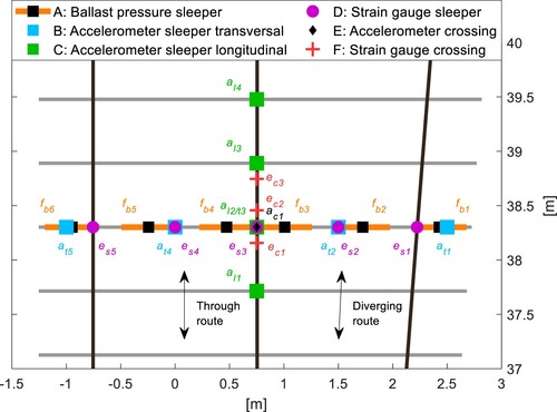
The strain gauges are oriented in the lengthwise direction of each body to measure the deformation due to vertical bending. The sampling rate is 2.4 kHz for these channels. The centrally located sleeper accelerometer $a_{l2/t3}$ is technically part of sensor group C but has an index for both longitudinal (l) and transversal (t) directions as these are of relevance when studying the structural response both along and across the track.

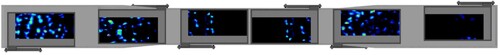
The six sleeper-ballast contact pressure sensors forming a Sensor Sleeper [26] are mounted under the sleeper (between the sleeper and the under sleeper pad). Each sensor has the dimensions 0.48 m × 0.21 m (length × width) giving a contact area of 0.1 m². Each sensor consists of a grid of small pressure sensors with dimensions 4.7 × 9.3 mm for a total of 2288 pixels per sensor. The sampling rate for these sensors is 100 Hz. The extent and centre of each sensor are indicated in Figure 2 by the line length and square, respectively. Pictures of the installation in track and a single sensor are shown in Figure 3. A view of the base of the full Sensor Sleeper with examples of pressure distribution results is presented in Figure 4. The contact from individual ballast stones is clearly visible in the results.

Figure 3. Sensor Sleeper in track (left) and individual sensor (right).

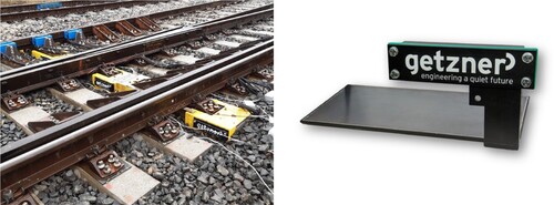
Figure 4. Illustration of the base of the Sensor Sleeper with overlayed example results for the six pressure sensors for traffic in the through route. The sensor positions correspond to Figure 2 with sensors $f_{b1}-f_{b6}$ counted from right to left. The brighter the colour the higher the contact pressure (black = zero pressure).

During the controlled locomotive run tests, four $(f_{b3}\text{to}{f}_{b6})$ out of the six sleeper-ballast sensors were recorded due to a temporary limitation in the number of measurement channels. Additional recordings for passages with a Taurus locomotive with similar axle load to the ER20 were made the day after with sensors $f_{b1}\text{to}{f}_{b4}$ at 80 km/h. Comparing the results for 80 and 120 km/h for the locomotive runs, it was concluded that the results were very similar in terms of the overall shape (the quasi-static response) and for the sensors with higher loads while the recordings at 120 km/h had more transient behaviour at lower loads. The results from the second day were therefore assumed to be representative, and the data from $f_{b5}$ and $f_{b6}$ in this dataset were added to the calibration set of data.

Rail geometry

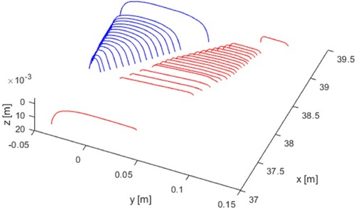
The crossing rail geometry was measured at several discrete cross-sections using a CALIPRI laser scanning device [27]. The section spacing was 50 mm in the transition area of the crossing. The measured geometry has been trimmed of excessive data to only leave the geometry relevant to represent the running surface, see Figure 5. In Simpack, the wing rail and the crossing rail are implemented as separate wheel-rail contact definitions defined by their measured discrete cross-sections. These 3D rail profile shapes are then generated via longitudinal spline interpolation, while the running surface of the stock rails and check rails are modelled using their nominal profiles.

Figure 5. Rail cross-sections for wing rail (right) and crossing nose (left) in the rail’s local coordinate system.

Simulation model

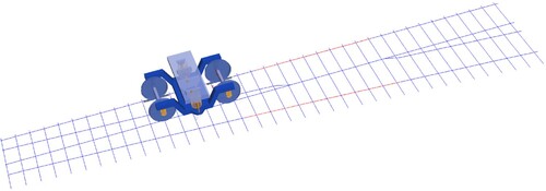
For the present investigation, the MBS model consists of a $\frac{1}{2}$ vehicle model, i.e. a bogie with half of the car body mass on top, and a finite element model representation of the crossing panel, see Figure 6. The vehicle and track models are truncated to save computational effort as the crossing transition is the primary focus. Here the length of the track model is 22 m. In Ref. [25], a convergence study was performed for a similar simulation case and it was shown that this track model length is sufficient and does not have any significant influence from the rail boundaries at the crossing transition. The model is initiated by finding the static equilibrium for each evaluated track configuration before the start of the time-domain simulation.

Figure 6. Illustration of crossing panel with bogie train model. Blue lines represent the track structure in the form of rails and sleepers. Red lines indicate check rails.

Track model

The track model is a two-layer finite element model where rails and sleepers are modelled with Timoshenko beam elements. The rail fastenings are represented with linear Kelvin bushing elements consisting of linear springs and dampers. The ballast and subgrade are represented by bi-linear springs in the vertical direction to represent potential voids between ballast and sleeper. The damping is modelled using linear viscoelasticity and is therefore active also when there is a gap. The track model of the crossing panel is implemented in the MBS code Simpack [28] using its non-linear flextrack module. The track model is generated using a Matlab [29] script that generates the necessary input bodies, bushing elements and track definition (.ftr) file for Simpack. This section will describe first the modelling of the rail and sleeper bodies, and then their assembly into a full crossing panel using force elements.

Rail and sleeper bodies

The finite element rail and sleeper bodies with a Timoshenko beam element discretization are first generated in the FE-program Abaqus [30] format (element type B31), and then condensed to substructures by employing the Craig–Bampton (CB) reduction scheme using the Abaqus *Substructure Generate command to meet the requirements of the non-linear flextrack module. A short summary of the aspects of the CB method of relevance for the paper will be given here. For full details, see Ref. [31] or a textbook such as Ref. [32]. The CB reduction starts from the undamped equations of motion for a body or substructure (1) $\mathit{M}\ddot{\mathit{u}}+\mathit{K}\mathit{u}=\mathit{f}$(1) where $\mathit{M}$ is the mass matrix, $\mathit{K}$ the stiffness matrix, $\mathit{u}$ the displacement field vector and $\mathit{f}$ is the vector of external nodal forces. The number of degrees of freedom (dofs) are reduced by first dividing $\mathit{u}$ into a partition $\mathit{u}=\left[\begin{array}{c}{\mathit{u}}^{\text{R}}\\ {\mathit{u}}^{\text{I}}\end{array}\right]$ where ${\mathit{u}}^{\text{R}}$ are the retained or boundary degrees of freedom and ${\mathit{u}}^{\text{I}}$ are the internal degrees of freedom where no external forces are acting. By doing so a relationship between $\mathit{u}$ and a reduced set of dofs $\mathit{p}$ can be established via a transformation matrix $\mathit{T}$, where the internal degrees of freedom ${\mathit{u}}^{\text{I}}$ are written as a function of the coordinate vector $\mathit{p}$ via a superposition of constraint modes and normal modes. The constraint modes are derived by applying a static unit displacement for each of the retained degrees of freedom while keeping the remaining retained dofs fixed. The normal modes are found by solving the eigenvalue problem when all retained degrees of freedom are fixed. In matrix form, the transformation is written as (2) $\mathit{u}=\left[\begin{array}{c}{\mathit{u}}^{\text{R}}\\ {\mathit{u}}^{\text{I}}\end{array}\right]=\left[\begin{array}{cc}\mathit{I}& 0\\ {\mathit{\Phi }}^{\text{C}}& {\mathbf{\Phi }}^{\text{N}}\end{array}\right]\left[\begin{array}{c}{\mathit{p}}^{\text{R}}\\ {\mathit{p}}^{\text{N}}\end{array}\right]=\mathit{T}\mathit{p}$(2) where ${\mathit{\Phi }}^{\text{C}}$ is a matrix where the columns are the constraint modes, and ${\mathit{p}}^{\text{R}}$ are the retained dofs that are thus identical to ${\mathit{u}}^{\text{R}}$. ${\mathit{\Phi }}^{\text{N}}$ is a matrix where the columns are a set of selected normal modes and ${\mathit{p}}^{\text{N}}$ are generalised modal coordinates. It is up to the user to choose what number of normal modes should be used in the reduction. In Simpack’s non-linear flextrack module, only the constraint modes are retained [9], which makes ${\mathit{\Phi }}^{\text{N}}$ empty and reduces the transformation relation to (3) $\mathit{u}={\mathit{T}}_{\text{C}}\mathit{p}=\left[\begin{array}{c}\mathit{I}\\ {\mathit{\Phi }}^{\text{C}}\end{array}\right]\mathit{p}$(3) This relationship will be used to transform the result outputs for the retained dofs to the full set of dofs for each substructure in the postprocessing of loading for individual rail and sleeper bodies. The reduced system of equations is then obtained by inserting Equation (3) into Equation (1), and multiplying with the transpose of ${\mathit{T}}_{\text{C}}$ from the left to obtain (4) $\begin{array}{rl}\hat{\mathit{M}}\ddot{\mathit{p}}+\hat{\mathit{K}}\mathit{p}& ={\mathit{T}}_{\text{C}}^{\text{T}}\mathit{f}\\ \text{where}\hat{\mathit{M}}& ={\mathit{T}}_{\text{C}}^{\text{T}}\mathit{M}{\mathit{T}}_{\text{C}}\text{and}\hat{\mathit{K}}={\mathit{T}}_{\text{C}}^{\text{T}}\mathit{K}{\mathit{T}}_{\text{C}}\end{array}$(4) The assembled structure and the different body types are presented in Figure 7. The crossing panel model consists of 38 sleeper and 13 rail substructures. Each sleeper is an individual substructure, while the rail substructures are assembled into continuous rails plus check rails when the model is imported into Simpack. The crossing panel rails are split into three longitudinal segments. There are four pieces of standard rail before the crossing, three along the distance occupied by the crossing (one crossing rail and two standard rails) and four after the crossing. In addition, there are two check rails that do not follow this division. This modular approach makes it easy to generate bodies with different discretization. In this case the discretization is finer for the crossing rail and the sleepers at the crossing transition. The details of the body properties and discretization are given in Table 1 and Figure 8.

Figure 7. Body types (substructures) and coordinate systems in the crossing panel. The z-axis is positive downwards.

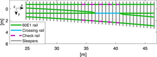
Figure 8. Variation in area moment of inertia for bending in the vertical plane (upper) and cross-section area (lower) for the crossing rail normalised by the constant properties of a 60E1 rail. Higher values correspond to sleeper locations.

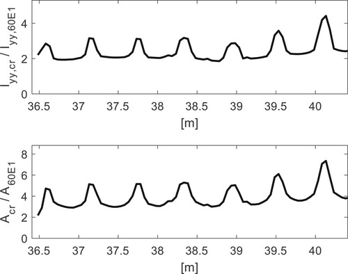
Table 1. Track body properties: $m$ is mass per metre length, $I$ area moment of inertia, $K$ transversal shear factor for Timoshenko beams, E Young’s modulus and $\nu$ Poisson’s ratio. The properties are given in coordinate systems with the same orientation as the track coordinate system (x longitudinal, y lateral and z vertical).

Body	Nominal values
60E1 rail	$m_{60E1}=60\text{kg}/\text{m}$$I_{\mathrm{yy},60E1}=30.3e-6{\text{m}}^4$$I_{\mathrm{zz},60E1}=5.1e-6{\text{m}}^4$$K_{\text{shear},60E1}=0.4$ [33]$E=210\text{GPa},\nu =0.3$
Crossing rail (average properties, see Figure 8 for details)	${\overline{m}}_{\text{cr}}=3.9m_{60E1}$${\overline{I}}_{yy,\text{cr}}=2.4I_{\mathrm{yy},60E1}$${\overline{I}}_{zz,\text{cr}}=54I_{\mathrm{zz},60E1}$${\overline{K}}_{\text{shear},\text{cr}}=0.6$
Check rail	$m_{\text{ch}}=40\text{kg}/\text{m}$$I_{yy,\text{ch}}=4.2e-6{\text{m}}^4$$I_{zz,\text{ch}}=2.8e-6{\text{m}}^4$$K_{\text{shear},\text{ch}}=0.4$
Sleepers	$m_{\text{sl}}=160\text{kg}/\text{m}$^a$I_{yy,\text{sl}}=2.6e-4{\text{m}}^4$^a$K_{\text{shear},\text{sl}}=0.82$^b$E=40\text{GPa},\nu =0.2$
Discretization and substructure settings for rails	FE beam element length is 0.075 m. Distance between retained nodes is 0.15 m for the crossing rail and 0.6 m for all other railsRetained nodal dofs: y and z translation for all nodes and y and z rotation at the end nodes for couplingLocked nodal dofs: x translation and x rotation
Discretization and substructure settings for sleepers	FE beam element length is maximum 0.2 m under the crossing rail and maximum 0.3 m away from the crossing rail. Each sleeper has 13–14 retained nodes along the crossing rail and 9–11 retained nodes away from the crossing rail depending on sleeper lengthRetained nodal dofs: z translation for all nodes and x rotation for check rail attachment nodesLocked nodal dofs: x translation and y and z rotations

^a Properties for nominal section. These are about 8% higher for 1 m of length towards each sleeper end.

^b Trapezoidal cross-section.

The degree of freedom settings for rail and sleepers in Table 1 report the dofs that are retained in the substructure generation (${\mathit{p}}^{\text{R}}$) and those that are locked and thus reduced from the equations of motion. The remaining dofs are internal and are recovered using Equation (3). For the rails, for example, the lateral and vertical degrees of freedom are retained while the displacement and rotation along the lengthwise direction are locked. Nodal rotations due to bending in the vertical and horizontal planes are internal except where they are needed for coupling between substructures and thus retained.

The variation in mass-moment of inertia and cross-section area for the crossing rail are presented in Figure 8. The locations where the crossing is stiffer and heavier correspond to the sleeper mounting positions. The properties have been computed from a CAD model of the crossing with a 50 mm spacing between the evaluated cross-sections. This lengthwise variation in properties is accounted for in the model.

The sleepers in the crossing panel have a wider base for 1 m in length towards each end of the sleeper. The bottom width is then 0.35 instead of 0.3 m. The slight increase in cross-section bending stiffness and area (∼8%) in this region is accounted for in the model.

Compared to the physical demonstrator, the model has several simplifications to ease modelling and reduce simulation costs. The sleepers are assumed to be perfectly orthogonal to the through route. In practice, they have a slight rotation with respect to the track centre line as a compromise between the through and diverging routes. The crossing rail beam elements are assumed to be perfectly parallel with the through route such that the lateral dofs of the beam elements are orthogonal to the through route. In the demonstrator, the long sleepers are split into two for the last sleepers in Figure 7 (i.e. beyond 45 m). Excluding this detail in the model is deemed an acceptable simplification as the focus lies on the crossing transition.

While the S&C demonstrator is located in a large radius curve that gives a radius of 3500 m for the through route, it is here modelled as a standard S&C with a straight-through route. At 120 km/h in a 3500 m curve with zero cant, a train will experience an average acceleration of 0.3 m/s². This would entail an increase in vertical wheel loads of a few per cent for the wheels going over the crossing transition, and a corresponding reduction on the stock rail. It would also entail a nominal lateral shift of the bogie by a few mm. Given that the expected error stemming from this model simplification is small, it was deemed justified as it simplifies the modelling significantly.

Force elements

The distribution of rail fastening and under sleeper pad (USP) stiffnesses based on their nominal properties are presented in Figure 9. The nominal ballast bed modulus and damping properties for all force elements are given in Table 2. These values are inspired by the calibrated properties from Ref. [18] where the ballast properties have been translated from line properties using a sleeper width of 0.3 m. The support stiffness is obtained by accounting for the ballast and USP stiffnesses in series while a single combined damping modulus is used to represent the damping in the ballast and USP layers.

Figure 9. Illustration of vertical stiffness distribution for under sleeper pads (USP) and rail fastenings in the crossing panel.

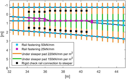
Table 2. Nominal ballast bed modulus and damping properties for elements in Figure 9.

Parameter	Nominal Value
Ballast bed modulus	$K_b$ = 67 kN/mm per m^2
Combined (support) ballast bed and USP damping modulus	$C_s$ = 167 Ns/mm per m^2
Damping for 25 kN/mm rail fastening	$c_{p,25}$ = 5 Ns/mm
Damping for 50 kN/mm rail fastening	$c_{p,50}$ = 10 Ns/mm

The rail fastenings are modelled using linear Kelvin bushing elements. The ballast stiffness is modelled using bi-linear bushing elements in the vertical direction as follows. For each sleeper, the vertical force $F_i$ in each ballast bushing element is computed as (5) $F_i=k_{\text{s},i}⟨u_i-g_i⟩+c_{\text{s},i}{\dot{u}}_i$(5) where $k_{\text{s},i}$ is the support stiffness and $c_{\text{s},i}$ the support damping, $u_i$ the vertical sleeper displacement and $g_i$ the gap at node i. The presentation is given for a single sleeper to avoid excessive indexing with sleeper number unless required. $⟨⟩$ is the Macaulay bracket defined as $⟨x-a⟩=\frac{1}{2}(x-a)+\frac{1}{2}|x-a|$. The Macaulay bracket is thus a ramp function that gives 0 for $a\ge x$ and $x-a$ for $x>a$. The support stiffness is computed using theory for springs in series accounting for the contribution from ballast stiffness and USP stiffness as (6) $k_{\text{s},i}=\frac{k_{\text{b},i}{k}_{\text{usp},i}}{k_{\text{b},i}+k_{\text{usp},i}}$(6) The ballast and USP stiffnesses for each bushing element are computed based on the sleeper surface area it represents. First, the ballast stiffnesses are computed from the ballast modulus $K_{\text{b}}$ as (7) $\begin{array}{rl}{k}_{\text{b},1}& =K_{\text{b}}{A}_1=K_{\text{b}}\frac{w(y_1)(y_2-y_1)}{2}\text{,}\text{for}i=1\\ k_{\text{b},i}& =K_{\text{b}}{A}_i=K_{\text{b}}\frac{w(y_i)(y_{i+1}-y_{i-1})}{2},2\le i\le N_r-1\\ k_{\text{b},N_r}& =K_{\text{b}}{A}_{N_r}=K_{\text{b}}\frac{w(y_{N_r})(y_{N_r}-y_{N_r-1})}{2},\text{for}i=N_r\end{array}$(7) where $y$ is the position along the sleeper, $w(y)$ is the width of the sleeper at this position and $N_r$ the number of nodes for sleeper r. The representative area $A_i$ for each bushing element is thus an average of the sleeper base areas between the present node and the adjacent nodes on each side. The fact that the sleeper end nodes only have a contact area on one side and should have a reduced stiffness is accounted for by the special cases for $i=1\text{and}{N}_r$. The USP contributions $k_{\text{usp},i}$ are computed analogously to $k_{\text{b},i}$ from the USP modulus $K_{\text{usp}}(y)$ that can vary along the sleeper according to Figure 9. The $c_{\text{s},i}$, which represents damping from ballast and USP, are computed analogously to $k_{\text{b},i}$ from the support damping modulus $C_{\text{s}}$.

In addition to the discrete damping provided by the bushing elements, the Simpack non-linear flextrack module allows for Rayleigh structural damping to be added to each flexible body. This damping was introduced to represent structural damping in the bodies themselves and to compensate for the lack of rotational damping from the rail fastenings as only translational dofs are included in the model. The Rayleigh damping coefficients were computed to give 1% of structural damping at 1 and 500 Hz, which is the frequency range of primary interest for the model. Due to the nature of Rayleigh damping it will be lower than 1% between those two boundary frequencies [32].

Sensor outputs

To compare the simulated and measured track responses, sensor signals from the simulations corresponding to the measured signals need to be computed. While the nodal displacements and hence the track displacement are readily available simulation outputs, the sleeper-ballast contact pressure and strains need to be computed in a postprocessing step.

Sleeper-ballast contact forces

The sleeper-ballast contact force at each sensor is computed as follows. From the bushing forces, the average sleeper-ballast contact pressure for the sleeper contact area represented by each bushing element is computed according to (8) ${\sigma }_i=\frac{F_i}{A_i}$(8) with $F_i$ and $A_i$ computed according to Equations (5) and (7). The sleeper-ballast contact pressure $\sigma (y)$ is assumed to vary linearly between the discrete bushing locations and can therefore be written as a superposition of ${\sigma }_i$ values multiplied by basis functions ${\beta }_i$ along the length of each sleeper as (9) $\sigma (y)=\sum _{i=1}^{N_r}{\sigma }_i{\beta }_i(y)$(9) The ${\beta }_i$ are linear triangular basis functions that are equal to one at node i and zero at nodes $i-1$ and $i+1$. The force at each pressure sensor k is computed from the pressure distribution via knowledge of the centre location $y_k$ and the length (a) and width (b) of the sensor (10) $F_k=b\underset{y_k-a/2}{\overset{y_k+a/2}{\int }}\sigma (y)\mathrm{dy}$(10) The integral is computed numerically using a trapezoidal integration scheme with 10 intervals along each sensor.

Strains

The strain outputs are computed via the bending moments of the bodies, which in turn are estimated via the beam element properties and the displacement field of each body. Taking the nodal displacements for each body and substructure, the full displacement and acceleration fields are recovered using the bodies’ coordinate transformation matrix ${\mathit{T}}_{\text{C}}$. The element matrices are exported from Abaqus and are reduced to only consider deformations in the vertical plane (z displacements and y and x rotations for rails and sleepers, respectively). Having extracted the relevant dof results, the nodal forces and torques can be computed directly from the element properties as (11) $\left[\begin{array}{c}\begin{array}{c}{F}_i\\ M_i\end{array}\\ \begin{array}{c}{F}_{i+1}\\ M_{i+1}\end{array}\end{array}\right]={\tilde{\mathit{M}}}_i\left[\begin{array}{c}\begin{array}{c}{\ddot{u}}_{z,i}\\ {\ddot{\psi }}_i\end{array}\\ \begin{array}{c}{\ddot{u}}_{z,i+1}\\ {\ddot{\psi }}_{i+1}\end{array}\end{array}\right]+{\tilde{\mathit{K}}}_i\left[\begin{array}{c}\begin{array}{c}{u}_{z,i}\\ {\psi }_i\end{array}\\ \begin{array}{c}{u}_{z,i+1}\\ {\psi }_{i+1}\end{array}\end{array}\right]$(11) where $F_i$ and $M_i$ are the nodal forces and moments, respectively, while ${\tilde{\mathit{M}}}_i$ and ${\tilde{\mathit{K}}}_i$ are the reduced element stiffness and mass matrices for element i. The inertia contribution to the results is very small compared to the stiffness contribution and can be omitted. There is no damping in the element formulation. As there are no external moments acting on the nodes of relevance for the present investigations, the bending moments are continuous in the regions of interest.

The bending strains are then computed from the nodal moments. For a Timoshenko beam, the change in cross-section rotation $\phi$ along the beam coordinate (x for crossing, y for sleeper) is related to the bending moment as [34] (12) $\frac{\mathrm{\partial \phi }}{\mathrm{\partial x}}(x)=-\frac{M(x)}{\mathrm{EI}(x)}$(12) The surface strain of the crossing rail or sleeper at discrete sensor locations is then computed as [34] (13) ${\epsilon }_{\mathrm{xx},k}=\frac{\mathrm{\partial \phi }}{\mathrm{\partial x}}(x_k)z_k$(13) where $z_k$ is the vertical distance from sensor k to the centre of mass of the cross-section at sensor location k. In the model, the sensor locations correspond to nodal locations so the strains can be computed directly from the nodal cross-section moments.

For a simply supported beam with different combinations of forces and moments applied, it has been verified that the bending moment recovery method is in perfect agreement with the analytical bending moment. For representative rail and sleeper bodies, it has also been verified that the substructure behaviour agrees with analytical beam theory in terms of deflection under load and for the first eigenfrequency.

Vehicle model

To represent the traffic load, the $\frac{1}{2}$ vehicle model based on the Manchester benchmark passenger vehicle [35] was adjusted to correspond to the ER20 locomotive axle load (20 tonnes) and bogie wheelbase (2.7 m). The vertical suspension properties were adjusted in proportion to the increase in car body mass to maintain resonance frequencies. A nominal S1002 wheel profile was used in the simulations.

Model calibration

The model calibration was performed for the 120 km/h locomotive run in the facing move of the through route. Then the validity of the calibration was verified using data from other speeds. The model calibration was performed in three steps. Firstly, an initial comparison was made between measurements and simulations to assess the areas where the model was inadequate. This was followed by a model parameterisation and sensitivity analysis to screen the influence of the different parameters. Finally, a calibration was performed by minimising the discrepancy between simulated and measured responses using an optimisation algorithm operating on a response surface description of the objective function.

Initial comparison of results

The model calibration started with a comparison between measurements and the nominal model setting with input data according to the track model section. In this comparison, good agreement was observed for the sensors at the crossing transition while there were greater discrepancies for the sensors towards the loaded stock rail. Figure 10 presents the vertical displacement of the crossing rail at the crossing transition (sensor a_c1), and the corresponding displacement for the point on the sleeper underneath the crossing transition (sensor a_l2/t3), see Figure 2 for sensor locations. It can be observed that the simulated displacement signatures agree well with the measured ones. The most significant difference is that the transient peaks at the crossing transitions are underestimated in the simulation model. Possible sources for this discrepancy that are unknown from the tests are differences in wheel profile and lateral contact position of the passing wheelset, and track irregularities that could give a different excitation at the crossing transition.

Figure 10. Comparison of measured and simulated vertical displacements at the crossing transition for crossing rail (a_c1) and sleeper (a_l2/t3). The measured displacements are reconstructed from accelerations.

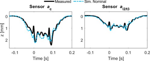
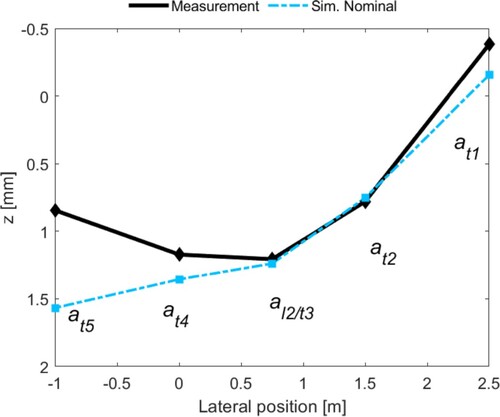
Figure 11 presents the sleeper deformation at the time of peak vertical displacement in measurement and simulation. It is observed that the simulation model predicts more sleeper rotation and less sleeper bending, and thus also a different sleeper bending moment distribution. The simulated behaviour with a predominately tilting sleeper is as expected for an S&C on a uniform ballast bed as previously reported in e.g. Ref. [36]. The discrepancy appears to be due to uneven ballast stiffness distribution under the sleeper at the installation site. This observation is also supported by the measured sleeper-ballast contact pressures that were low underneath the crossing. A snapshot of the sleeper-ballast contact pressures under load can be observed in Figure 4, while time histories are reported in the Results section, see Figure 21. The subsequent calibration therefore concerns the void distribution under the crossing transition sleeper, the global ballast stiffness, and the rail fastening stiffness as these are the track properties with the greatest uncertainties compared to the rail and sleeper bodies.

Figure 11. Deformation of the crossing transition sleeper in measurement and simulation at peak displacement. The measured displacements are reconstructed from accelerations. See Figure 2 for sensor locations.

Model parameterisation

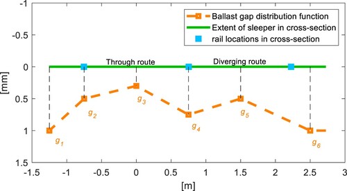
The ballast and rail fastening stiffnesses are parameterised in the model. The ballast was parameterised using local parameters for gaps $g_p$ under the sleeper at the crossing transition and one global ballast stiffness scaling parameter for the whole track model (h₁). The two rail fastening stiffnesses, see Figure 9, are parameterised by a stiffness scaling parameter (h₂). The parameters are gathered in the vector h. An overview of the ballast parameterisation is given in Figure 12. The void parameter distribution is presented in Figure 13.

Figure 12. Ballast parameterisation domains in the crossing panel.

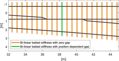
Figure 13. Detail of ballast gap parameterisation. The ballast gap distribution is described by a piecewise linear function determined by six gap variables g_p at the shown locations. The gap distribution in the figure is arbitrary for illustration purposes.

Objective function

The agreement between measured and simulated signals is quantified by computing the root mean square (RMS) value of the difference between the signals at each measurement point and then normalising by the RMS of the sum of signals in each sensor group. For a studied bogie passage, let ${\mathit{s}}_{\mathrm{gk}}$ be the vector of values recorded for sensor number k in sensor group g. The sensor groups are illustrated in Figure 2. Let ${\hat{\mathit{s}}}_g$ be the sum of signals ${\mathit{s}}_{\mathrm{gk}}$ for each sensor group with $N_g$ sensors. The agreement between measurements and simulation for each sensor can then be computed as (14) $p_{\mathrm{gk}}=\frac{\text{rms}({\mathit{s}}_{gk,\text{mea}}-{\mathit{s}}_{gk,\text{sim}})}{\text{rms}({\hat{\mathit{s}}}_{g,\text{ mea}})}$(14) The objective function P measuring the overall goodness of fit is then computed as (15) $P=\sum _{g=A}^{g=F}\sum _{k=1}^{N_g}{w}_g{p}_{\mathrm{gk}}$(15) where sim and mea correspond to simulation and measurement, respectively and $w_g$ are scaling factors for each sensor group. In the analysis all $w_g$ were set equal to one except for $w_C$ that was increased to four in the calibration step. The motivation for this is given in the calibration section. The compared signals have been shifted in time to overlap and interpolated to have the same time discretization.

Sensitivity analysis

A sensitivity analysis was performed to verify that (1) all parameters are identifiable in the sense that they have a significant and unique influence on the structural response, and (2) to identify the parameter region of interest for a more precise calibration.

The analysis was performed by generating a set of Latin Hypercube Samples (LHS) [37] consisting of 500 parameter sets where each set is a randomised combination of parameter values drawn from the defined parameter ranges. The size of the LHS sample is motivated by the high dimensionality of the problem with eight parameters. Each parameter set constitutes the input to one simulation run that gives the crossing panel sensor response for the given parameter setting. The parameter ranges are given in Table 3 and Figure 15. The discrepancy between measurement and simulation according to Equations (14) and (15) was computed for all 500 runs.

Table 3. Ballast and rail fastening stiffness in the calibration process.

Parameter	Range in sensitivity analysis	Range in calibration	Calibrated value
Ballast stiffness scaling $h_1$	0.5–2.5	1.5–2.5	1.79 (equivalent to a bed modulus of 120 MPa/m^2)
Rail fastening stiffness scaling $h_2$	0.75–2.5	1–1.6	1.23 (equivalent to a rail fastening stiffness of 30.75 kN/mm)

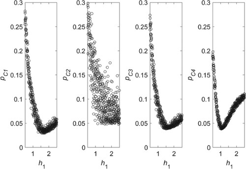
From the sensitivity analysis, by studying correlation plots between the parameters and objectives, it was concluded that the global ballast stiffness was the most influential parameter. It was also concluded that all parameters had a significant influence on the objectives even though the influence of $g_6$ was minor as it represents the ballast gap far out on the unloaded side of the track. Figure 14 presents $p_{\mathrm{Ck}}$ for the sleeper-mounted accelerometers underneath the crossing rail as a function of the global ballast stiffness. Each circle corresponds to one LHS sample and simulation. It can be observed that the response for sensor $a_{l2/t3}$ ($p_{C2}$) has greater variability due to the variability in the six gap parameters, while the influence of global ballast stiffness on the other sensors is more distinct.

Figure 14. Objective function values $p_{\mathrm{Ck}}$ comparing measured and simulated displacements for sensor group C (sleeper accelerometers along the crossing) as a function of the ballast stiffness scaling parameter $h_1$. The measured displacements are reconstructed from accelerations.

Calibration

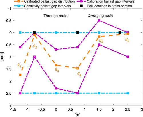
Based on the results from the sensitivity study, the parameter ranges were reduced for the calibration step according to Table 3 and Figure 15. The range for the global ballast stiffness was determined from the responses of $p_{C1}$ and $p_{C3}$ in Figure 14 as they are adjacent to the instrumented sleeper, while the range for the other parameters was determined from the 10 runs with the lowest global objective in the chosen range of global ballast stiffness scaling. The lower end of the range for ballast gap $g_5$ was extended to negative values compared to the sensitivity study as all of the best solutions were found close to the zero boundary. A negative gap value would correspond to a local elevation in the ballast layer at that point giving a pre-load in the ballast bushing element at zero displacement. The calibration step was performed by first evaluating a new LHS sample of 500 runs with the narrower parameter band. In addition, all boundary points on the parameter ranges were evaluated giving 2⁸ = 256 additional runs for a total of 756.

Figure 15. Ballast gap parameter ranges in different steps of the calibration.

Then a response surface described by a polyharmonic spline denoted $\hat{P}({\mathit{h}}_m)$ was fitted to the simulated objective function values $P({\mathit{h}}_m)$ using the software library [38]. Polyharmonic splines are particularly well suited to fit functions of higher dimensionality but require good resolution on the parameter boundaries [39].

The accuracy of the response surface fit was evaluated by fitting the spline to subsets of all runs and then use the remaining runs as a validation set. For this analysis, 75 random samples of 75 runs each were removed from the full pool of 756 runs, whereafter the response surface was fitted to the remaining 681 results. The average difference between $P({\mathit{h}}_m)$ and $\hat{P}({\mathit{h}}_m)$ for the remaining 75 parameter settings in the validation set was within 1%, while the maximum difference considering all the evaluated combinations of response surface and validation sets was 5.5%. These results indicate that the response surface represented the objective function very well and that the calibration could be performed using the response surface, thus alleviating the need to perform further simulations in the calibration process.

A gradient-based optimisation method in the form of fmincon in Matlab R2021 [29], using the interior-point algorithm, was applied to find the minimum of the objective function as described by the response surface. Given the low computational effort to evaluate the response surface, 1000 randomised starts on the parameter space were used in the evaluation and the lowest optimum found among these repeated optimisations is assumed to be the global optimum. During initial optimisation trials, it was found that increased weight was needed for sensor group C (sleeper accelerometers along the crossing). Due to the large number of sensors along the crossing transition sleeper and the corresponding weight given to these responses in the objective function, optima were found where these sensors had a good agreement at the compromise of sensor group C where sensors $a_{l1}$, $a_{l3}$ and $a_{l4}$ are the best independent measures of the global ballast stiffness. Therefore, a weight factor of $w_C=4$ was chosen to ensure that the sleeper displacements in sensor group C are in good agreement with measurements and that a realistic global ballast stiffness is obtained.

The final objective function is presumed to be convex as all starts converged to the same optimum which is then assumed to be the global optimum. The calibrated parameter set is found in Table 3 and Figure 15. It can be observed that the calibrated values are well inside the intervals of the reduced parameter ranges. This suggests that the parameter range was generous enough to not exclude any optima.

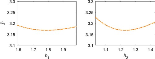
The sensitivity of the objective function $\hat{P}$ around the global optimum was evaluated for one parameter at a time. The results are presented Figure 16 for the ballast gaps and in Figure 17 for the stiffness scaling parameters. The ballast gaps are plotted for ±0.25 mm around the optimum and the stiffness scaling parameters for ±20%. It can be observed among the ballast gap parameters that $g_5$ has the greatest sensitivity and $g_6$ the lowest.

Figure 16. Influence on $\hat{P}$ from individual ballast gap parameters around the global optimum.

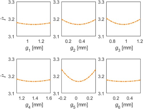
Figure 17. Influence on $\hat{P}$ from individual stiffness scaling parameters around the global optimum.

Results

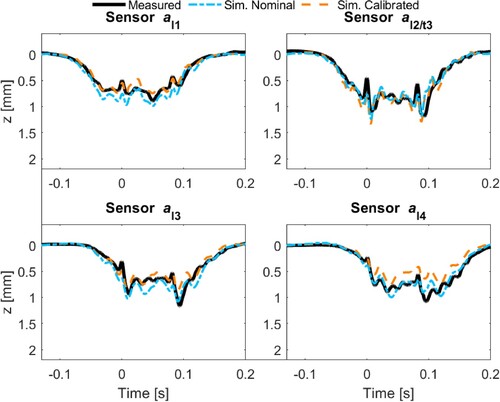
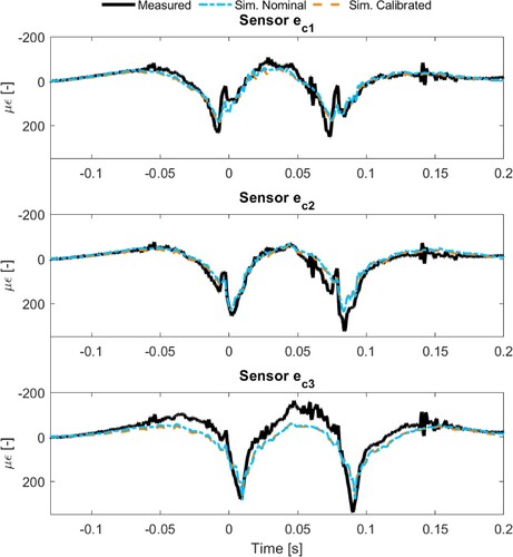
In the following, sensor responses from measurements and simulations with nominal and calibrated models are plotted. Figure 18 presents displacements and strains for the densely instrumented sleeper under the crossing transition. It can be observed that the calibration has significantly improved the agreement for the strains. In particular, this is true for sensor $e_{s2}$ where the tension in the upper surface of the sleeper has changed to the compression observed in the measurements. The displacements on the other hand have not improved and are even slightly worse for some channels. Figure 19 presents the sleeper displacements along the crossing. For these signals, the agreement was good from the start and no significant changes have been made from the calibration.

Figure 18. Displacements and strains for the sleeper at the crossing transition. Results from measurements and from nominal and calibrated models. See Figure 2 for sensor locations.

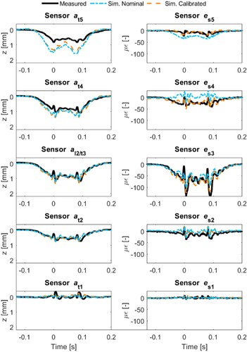
Figure 19. Displacements for sleepers along the crossing rail. Results from measurements and from nominal and calibrated models. See Figure 2 for sensor locations.

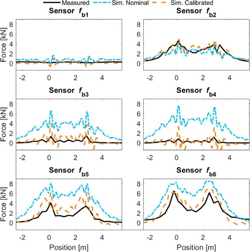
The crossing rail and sleeper displacements at the crossing transition are compared in Figure 20, while the crossing strains are presented in Figure 21. For these results, the nominal and calibrated models are similar as well and close to the measured. To summarise, the calibration for the crossing and sleeper displacements and strains has primarily given a better agreement for the sleeper strains, while the remaining channels remain about the same. The most significant difference between nominal and calibrated models can be seen for the sleeper-ballast contact pressure in Figure 22. The calibrated model has much better agreement, and in particular for force sensors 3 and 4 close to the crossing transition. By evaluating the sum of all ballast force signals, it can also be concluded that the instrumented sleeper under the crossing transition carries less total load at the sensor locations on the voided ballast bed compared to the results that would be expected if the ballast properties were uniform. The distribution of sleeper-ballast contact forces is in good physical agreement with the changes in sleeper strain from the nominal to the calibrated model given that beam theory would predict this change with a weaker support at the centre of the track.

Figure 20. Displacements for sensors a_l2 and a_c to compare sleeper and crossing rail displacement at the crossing transition. Results from measurements and from nominal and calibrated models. See Figure 2 for sensor locations.

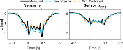
Figure 21. Crossing rail strains. Results from measurements and from nominal and calibrated models. See Figure 2 for sensor locations.

While the calibration significantly improved the agreement between measurement and simulation, good agreement was not found for all signals, primarily for the sleeper displacement towards the loaded stock rail. The reasons for this are not fully understood and there are several factors that could contribute to what appears to be either an inconsistency or lack of information from the measurement data, or an insufficient parameterisation of the model to meet all measured signals.

One reason could be that the ballast support conditions are not fully known even though the sleeper was densely instrumented. The sensors cover 45% of the bottom surface and it has been assumed that this part of the sleeper surface is representative for the full sleeper. It is also assumed that the gap distribution between sleeper and ballast can be described with a piecewise linear function determined by six parameters. The measured displacements also have a level of uncertainty as they are reconstructed from measured accelerations. Even though they showed good qualitative agreement with potentiometer measurements relative to the ballast bed, the absolute level of displacement has some uncertainty.

To evaluate the robustness of the calibrated model, it was simulated for, and compared to, the measurement results for 60 and 80 km/h. It was found that the goodness of fit was still good as the objective function values were of similar magnitudes.

Figure 22. Sleeper-ballast contact forces. Results from measurements and from nominal and calibrated models. See Figure 2 for sensor locations.

Summary and conclusions

A structural track model of a crossing panel for implementation in MBS simulations has been presented. The model accounts for the flexibility of rails and sleepers and bi-linear ballast stiffness at selected sleepers. In addition to the model, postprocessing steps have been developed for the extraction of the structural loading in terms of bending moments and sleeper-ballast contact pressures.

The model has been validated via calibration to measurement data from a comprehensively instrumented S&C demonstrator. It was shown that the presented MBS model can represent the dynamic structural response well after calibration of physical ballast and rail fastening parameters. Even though only one crossing panel has been studied here, it demonstrates how uneven the ballast support conditions can be and that this influences the structural loading. It was necessary to introduce a position-dependent ballast gap function to obtain good agreement between measurement and simulations. While the calibration significantly improved the agreement between measurement and simulations, it was not possible to obtain full agreement for all signals, primarily for the sleeper displacements towards the loaded stock rail. The exact reason for this has not been identified and remains a topic for further studies.

The calibration procedure using LHS samples to explore the parameter space, and a final calibration based on a gradient-based method on a polyharmonic spline fit to the LHS responses, worked well. The calibration optimisation problem was found to be smooth and predominately convex.

Disclosure statement

No potential conflict of interest was reported by the author(s).

Additional information

Funding

This work was supported by the Horizon 2020 Framework Programme in the Shift2Rail projects In2Track2 and In2Track3 [grant numbers 826255, 101012456]. The computations and data handling were enabled by resources provided by the National Academic Infrastructure for Supercomputing in Sweden (NAISS) and the Swedish National Infrastructure for Computing (SNIC) at C3SE partially funded by the Swedish Research Council through grant agreements no. 2022-06725 and no. 2018-05973.

References

- In2Track. Deliverable 2.2 enhanced S&C whole system analysis, design and virtual validation (final); 2020.
- Wang P, Xu JM, Xie KZ, et al. Numerical simulation of rail profiles evolution in the switch panel of a railway turnout. Wear. 2016 Nov 15;366-367:105–115. doi:10.1016/j.wear.2016.04.014
- Johansson A, Pålsson B, Ekh M, et al. Simulation of wheel-rail contact and damage in switches & crossings. Wear. 2011 May 18;271(1-2):472–481. doi:10.1016/j.wear.2010.10.014
- Skrypnyk R, Ossberger U, Pålsson BA, et al. Long-term rail profile damage in a railway crossing: field measurements and numerical simulations. Wear. 2021 May 15;472:203331.
- Li X, Ekh M, Nielsen JCO. Three-dimensional modelling of differential railway track settlement using a cycle domain constitutive model. Int J Numer Anal Met. 2016 Aug 25;40(12):1758–1770. doi:10.1002/nag.2515
- Six K, Sazgetdinov K, Kumar N, et al. A whole system model framework to predict damage in turnouts. Vehicle Syst Dyn. 2023;61(3):871–891.
- Bezin Y, Pålsson BA. Multibody simulation benchmark for dynamic vehicle-track interaction in switches and crossings: modelling description and simulation tasks. Vehicle Syst Dyn. 2023;61(3):644–659.
- Pålsson BA, Ambur R, Sebes M, et al. A comparison of track model formulations for simulation of dynamic vehicle-track interaction in switches and crossings. Vehicle Syst Dyn. 2023;61(3):698–724.
- Systemes D. Simpack FlexTrack learning module: Dassault Systemes; 2022. [cited 2022 Nov 11]. Available from: https://eduspace.3ds.com/
- Kassa E, Nielsen JCO. Dynamic train-turnout interaction in an extended frequency range using a detailed model of track dynamics. J Sound Vib. 2009 Mar 6;320(4-5):893–914. doi:10.1016/j.jsv.2008.08.028
- Grossoni I, Bezin Y, Neves S. Optimisation of support stiffness at railway crossings. Vehicle Syst Dyn. 2018;56(7):1072–1096. doi:10.1080/00423114.2017.1404617
- Alfi S, Bruni S. Mathematical modelling of train-turnout interaction. Vehicle Syst Dyn. 2009;47(5):551–574. doi:10.1080/00423110802245015
- Jorge PFM. Modelling and enhancing track support through railway switches & crossings. Huddersfield: University of Huddersfield; 2020.
- Chen JY, Wang P, Xu JM, et al. Simulation of vehicle-turnout coupled dynamics considering the flexibility of wheelsets and turnouts. Vehicle Syst Dyn. 2023;61(3):739–764.
- Hamarat M, Papaelias M, Silvast M, et al. The effect of unsupported sleepers/bearers on dynamic phenomena of a railway turnout system under impact loads. Appl Sci-Basel. 2020;10(7):2320.
- Grossoni I, Le Pen LM, Jorge P, et al. The role of stiffness variation in switches and crossings: comparison of vehicle-track interaction models with field measurements. P I Mech Eng F-J Rai. 2020 Nov;234(10):1184–1197.
- Otorabad HA, Bezin Y, Grossoni I, et al. Finite element analysis of a crossing panel under dynamic moving load – effect of support conditions and implications on foot fatigue. P I Mech Eng F-J Rai. 2023 May;237(5):563–575.
- Milosevic MDG, Pålsson BA, Nissen A, et al. Condition monitoring of railway crossing geometry via measured and simulated track responses. Sensors-Basel. 2022;22(3):1012.
- Bruni S, Anastasopoulos I, Alfi S, et al. Effects of train impacts on urban turnouts: modelling and validation through measurements. J Sound Vib. 2009 Jul 24;324(3-5):666–689. doi:10.1016/j.jsv.2009.02.016
- Torstensson PT, Squicciarini G, Kruger M, et al. Wheel-rail impact loads and noise generated at railway crossings – influence of vehicle speed and crossing dip angle. J Sound Vib. 2019 Sep 15;456:119–136. doi:10.1016/j.jsv.2019.04.034
- Liu X, Markine VL, Wang H, et al. Experimental tools for railway crossing condition monitoring (crossing condition monitoring tools). Measurement (Mahwah N J). 2018 Dec;129:424–435. doi:10.1016/j.measurement.2018.07.062
- Ossberger U, Kollment W, Eck S. Insights towards condition monitoring of fixed railway crossings. Procedia Struct Integr. 2017;4:106–114. doi:10.1016/j.prostr.2017.07.007
- Boogaard MA, Li Z, Dollevoet RPBJ. In situ measurements of the crossing vibrations of a railway turnout. Measurement (Mahwah N J). 2018 Sep;125:313–324. doi:10.1016/j.measurement.2018.04.094
- Shih JY, Weston P, Entezami M, et al. Dynamic characteristics of a switch and crossing on the West Coast main line in the UK. Railway Eng Sci. 2022 Jun;30(2):183–203. doi:10.1007/s40534-021-00269-4
- Milosevic MDG, Pålsson BA, Nissen A, et al. Reconstruction of sleeper displacements from measured accelerations for model-based condition monitoring of railway crossing panels. Mech Syst Signal Process. 2023;192:1–21.
- Loy H, Kessler M, Augustin A, et al. Switches & crossings: defined elasticity for new turnout designs. Rail Eng Int. 2022;1:5–9.
- CALIPRI C4X measurement device. Available from: https://www.nextsense-worldwide.com/en/
- Simpack. Version 2022x.4: Dassault Systemes; 2022. Available from: 3ds.com
- Matlab R2021. The Matworks Inc.
- Abaqus. Dassault Systemes; 2018.
- Craig RR, Bampton MCC. Coupling of substructures for dynamic analyses. AIAA J. 1968;6(7):1313. doi:10.2514/3.4741
- Craig RR, Kurdila AJ. Fundamentals of structural dynamics. 2nd ed.. Hoboken, New Jersey, U.S.A.: John Wiley; 2006.
- Shih J-Y, Kostovasilis D, Bezin Y, et al., editors. Modelling options for ballast track dynamics. 24th International Congress on Sound and Vibration (ICSV24); London, UK; 2017.
- Carrera E, Giunta G, Petrolo M. Beam structures: classical and advanced theories. 1st ed. Hoboken: John Wiley; 2011.
- Iwnicki S. Manchester benchmarks for rail vehicle simulation. Vehicle Syst Dyn. 1998 Sep;30(3-4):295–313. doi:10.1080/00423119808969454
- Li X, Nielsen JCO, Pålsson BA. Simulation of track settlement in railway turnouts. Vehicle Syst Dyn. 2014;52:421–439. doi:10.1080/00423114.2014.904905
- Olsson A, Sandberg G, Dahlblom O. On Latin hypercube sampling for structural reliability analysis. Struct Saf. 2003;25(1):47–68. doi:10.1016/S0167-4730(02)00039-5
- Wiens T. Radial basis function network. MATLAB Central File Exchange; 2022.
- Fasshauer GF. Meshfree approximation methods with MATLAB. Singapore: World Scientific; 2007.