Dynamic vehicle–track interaction and structural loading in a crossing panel – calibration and assessment of a model with a 3D representation of the crossing rail

Abstract

A three-dimensional (3D) finite element model of a railway crossing panel for use in multibody simulation (MBS) of dynamic vehicle–track interaction is presented. It is a two-layer track model with stock rails and sleepers represented by beam elements and a crossing rail represented by 3D solid elements. The track model uses linear bushings for the rail fastenings and bi-linear bushings for the ballast to allow for potentially voided sleepers. Based on the output from the MBS, the structural loading of the crossing in terms of strains, stresses and sleeper-ballast contact pressures is extracted in a post-processing step. The model is calibrated and validated to measurement data from a comprehensively instrumented switch & crossing (S&C) demonstrator installed in the Austrian railway network as a part of the European research programme Shift2Rail. The applied procedure for the calibration and critical assessment of the crossing model is described in detail. It is based on a model parameterisation with eight parameters relating to the rail fastening and foundation stiffnesses and to a distribution of the ballast voids. The calibration method uses Latin hypercube samples to explore the parameter space in a sensitivity analysis before a parameter optimisation is performed using a gradient-based method on a response surface built from a polyharmonic spline. In a comparative study it is shown that the 3D model and a more conventional beam model of the crossing rail show similar calibration results and good agreement with the measured data. The 3D model allows for the extraction of stress concentrations in the crossing rail but has an increased computational time of about 30% compared to the beam model.

Keywords:

• Railway
• switches & crossings
• turnout
• 3D finite element model
• multibody simulation
• dynamic vehicle–track interaction

1. Introduction

A fixed crossing allows for trains to cross intersecting tracks. In the wheel transfer from wing rail to crossing nose (or vice versa), the conicity of the wheel in combination with the variation in rail geometry along the crossing results in a wheel–rail excitation that is characterised by a dip in the vertical wheel trajectory. This leads to wheel–rail impact loading and subsequent damage of the running surfaces of wheels and rails (plastic deformation, rolling contact fatigue and wear), noise and vibration, and differential settlement of the supporting foundation. It can also lead to rail fatigue due to bending and sleeper cracking if the crossing is not maintained properly. The focus of this paper is on the calibration of a model of the crossing panel, the part of the turnout where the impact loading takes place, see Figure 1. The beam model of the crossing panel that was developed in [1] is extended in this paper to include a 3D representation of the crossing rail to obtain a more detailed understanding about the structural loading of the crossing rail. As a part of the European Research programme Shift2Rail, a comprehensively instrumented S&C demonstrator has been installed in the Austrian railway network. It has design features such as softer rail pads to reduce impact loading and improve S&C long-term performance. The data from this measurement campaign is presented in detail in [2].

Figure 1. Illustration of a crossing panel within a turnout.

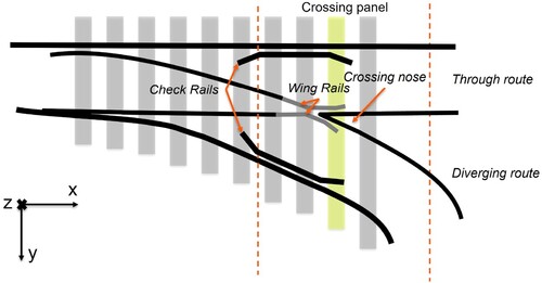
In [2], the model was calibrated against measured track responses from the Austrian demonstrator. In the calibration, a parameterisation of the void distribution below the sleeper under the crossing nose (sleeper highlighted in yellow in Figure 1) and the stiffnesses of rail fastenings and ballast was introduced to model the support conditions in the field. The calibration of the beam model was based on the minimisation of an objective function comprising a weighted sum of the root mean square error between the measured and simulated displacements, strains and sleeper–ballast contact forces. It was concluded that the agreement between simulation and measurement could be improved by enhanced detail of the crossing rail model, especially for local strains in the crossing rail that are difficult to estimate with beam theory. In this paper, the track model has been enhanced by modelling the crossing rail using 3D solid elements to enable detailed calculation of the stress and strain fields. The objective is to use the model in a holistic optimisation of the crossing panel. This requires a detailed model which can account for many different damage mechanisms that are relevant for the crossing panel, while keeping a computational effort that facilitates optimisation of the design.

Structural track models of S&Cs can be found in several previous studies using different methods, commonly representing the rails by beam elements [3–7]. With this method, a reasonable computational time can be achieved while still allowing to evaluate the structural response of the S&C. In [8], a reduced track model based on modal decomposition was implemented in a multibody simulation (MBS) software. It was applied for a plain track case with prescribed track irregularities accounting for dynamic modes up to 3 kHz. However, this track model was dismissed for use in S&C simulations due to high computational effort. Another, generally more computationally demanding approach is to use a 3D finite element model for the entire crossing panel, where the distributions of stress and strain can be determined without post-processing steps. This type of modelling has been compared to the modal decomposition method in [9]. For four sleeper bays on either side of the crossing nose, the turnout was modelled with 3D solid elements, while beam elements were used outside of this range and the loading was calculated from a simplified analytical model. In [10], 4.5 m of the crossing panel and one wheelset were modelled using 3D solid finite elements. A similar approach was used in [11]. However, here a pre-calculated contact load history describing the dynamic interaction between a moving unsprung wheelset mass and the flexible track was taken from another model and applied to the 3D finite element model to reduce computational cost.

In addition to proper modelling of vehicle, rails and sleepers, the understanding and simulation of realistic support conditions in switches and crossings are crucial to accurately evaluate the performance of the crossing panel. Commonly, the track stiffness is calibrated against measured accelerations. In [7], track stiffness was calibrated against accelerometer data to provide the same point receptance on the crossing nose. Similarly, in [12], the support conditions along a turnout were studied through field measurements and simulation. In that study, the ballast support was calibrated using displacements reconstructed from geophone measurements revealing a low local ballast support under the crossing nose. In [13], a model calibration by brute force grid search optimisation was performed using seven track stiffness parameters to fit the simulation model against measured vertical sleeper accelerations. After calibration of six studied turnouts, four of the models were indicating one or more voided sleepers in the crossing panel.

In this paper, a computationally efficient structural finite element model of a crossing panel for use in MBS software is presented and calibrated. In Chapter 2, the track and vehicle models are described, as well as the substructuring method used for the FE models. Chapter 3 introduces a calibration method that efficiently deals with the multi-dimensional calibration optimisation problem while providing detailed information about the influence of each parameter on the objective function. A brief summary of the field measurements presented in [2] is also given. In Chapter 4, the calibrated model is presented and in Chapter 5 the 3D simulation model is demonstrated and compared with the measurements and the less detailed beam model. In Chapter 6, the conclusions of the paper are presented.

2. Simulation model

The structural finite element model of the crossing panel is implemented in the commercial MBS software Simpack using substructures generated from individual finite element models of the crossing rail, stock rails and sleepers. The vehicle model is based on the Manchester benchmark passenger vehicle model [14]. For each evaluated track configuration, the initial conditions of the vehicle and track models are determined by evaluating the static equilibrium for the vehicle–track system before the start of each time-domain simulation. The sampling frequency of the time integration is 2500 Hz. The simulation model is described in detail in the following sections.

2.1. Track and vehicle models

The model of the crossing panel consists of 37 sleeper bays. In [15], a convergence study was performed for a similar simulation case and it was shown that this track model length is sufficient and does not lead to any significant influence from the rail boundaries on track responses evaluated near the crossing nose. The track model consists of two layers with stock rails and sleepers modelled using Timoshenko beams while the crossing rail uses 3D solid elements. The crossing nose and wing rail geometry has been measured using a CALIPRI laser scanning device [16] at a number of discrete cross-sections. The spacing between each measured cross-section is 50 mm in the transition area of the crossing. Using this data, the wing rail and crossing nose are implemented in Simpack as separate wheel–rail contact definitions. From the discrete cross-section data, the 3D rail profile shapes are generated via longitudinal spline interpolation. All other rails are modelled using their nominal running surface profile.

To account for the rotational stiffness (about the x-axis) of each rail fastening in the 3D crossing rail model, each rail fastening is modelled as two Kelvin–Voigt bushing elements using force elements in Simpack with different y-coordinates (see Figure 1 for coordinate system) to provide the vertical stiffness and rotational stiffness of a physical rail pad. For the other rails, each rail fastening is modelled using one bushing element with stiffnesses in longitudinal, lateral and vertical directions but with no rotational stiffnesses. The combined vertical stiffness of the ballast and under sleeper pads is modelled with bi-linear springs to represent potential voids between sleeper and ballast. The damping is modelled using linear dampers resulting in a damping force regardless of whether or not the sleeper is currently supported. The combined ballast and under sleeper pad support stiffness is calculated as for two springs in series (1) $k_{\mathrm{s},i}=\frac{k_{\mathrm{b},i}{k}_{\mathrm{usp},i}}{k_{\mathrm{b},i}+k_{\mathrm{usp},i}}$(1) The ballast and under sleeper pad stiffnesses are computed to represent a certain section of sleeper base area. These are calculated identically aside from that the under sleeper pad bed modulus varies depending on both lateral and longitudinal positions within the crossing panel, while the ballast bed modulus $K_{\mathrm{b}}$ is assumed to be uniform for the entire turnout. The ballast stiffnesses are calculated as (2) $\begin{array}{ll}{\displaystyle k_{\mathrm{b},1}=K_{\mathrm{b}}{A}_1=\frac{K_{\mathrm{b}}B\left(y_1\right)(y_2-y_1)}{2},}& \mathrm{for}i=1\\ \\ {\displaystyle k_{\mathrm{b},i}=K_{\mathrm{b}}{A}_i=\frac{K_{\mathrm{b}}B\left(y_i\right)(y_{i+1}-y_{i-1})}{2},}& 2\le i\le N_r-1\\ \\ {\displaystyle k_{\mathrm{b},N_r}=K_{\mathrm{b}}{A}_{N_r}=\frac{K_{\mathrm{b}}B\left(y_{N_r}\right)(y_{N_r}-y_{N_r-1})}{2},}& i=N_r\end{array}$(2) where $B\left(y\right)$ is the width of the sleeper at lateral coordinate y and $N_r$ is the number of nodes for sleeper r. The support damping $c_{s,i}$ is calculated in the same manner using the support damping modulus $C_s$. In addition to the discrete damping from the rail fastenings and supporting foundation, Rayleigh damping is added to each rail and sleeper body when implemented in Simpack. The Rayleigh coefficients have been computed by solving the system of equations in (3(3) $\left[\begin{array}{cc}1& {\omega }_m^2\\ 1& {\omega }_n^2\end{array}\right]\left[\begin{array}{c}\alpha \\ \text{β}\end{array}\right]=\left[\begin{array}{c}2{\xi }_m{\omega }_m\\ 2{\xi }_n{\omega }_n\end{array}\right].$(3) ) to give 1% of structural damping at the boundaries of the primary frequency range of the model, 1 and 500 Hz [17], i.e. ${\xi }_m={\xi }_n=0.01$, ${\omega }_m=1$ Hz and ${\omega }_n=500$ Hz. (3) $\left[\begin{array}{cc}1& {\omega }_m^2\\ 1& {\omega }_n^2\end{array}\right]\left[\begin{array}{c}\alpha \\ \text{β}\end{array}\right]=\left[\begin{array}{c}2{\xi }_m{\omega }_m\\ 2{\xi }_n{\omega }_n\end{array}\right].$(3) The vertical force $F_i$ from the support acting on the crossing sleeper at node i is calculated as (4) $F_i=k_{\mathrm{s},i}〈u_i-g_i〉+c_{\mathrm{s},i}{\dot{u}}_i,$(4) where $u_i$ is the vertical sleeper displacement, $k_{\mathrm{s},i}$ the support stiffness, $c_{\mathrm{s},i}$ the support damping, while $g_i$ is the gap between sleeper and ballast at node i. The Macaulay brackets denoted with $〈〉$ are defined as $〈u-g〉=\frac{1}{2}(u-g)+\frac{1}{2}|u-g|$ resulting in a step function which is 0 for $g\ge u$ and u−g for u>g.

The vehicle model used in this study is a model of one bogie with an added rigid mass representing half of the car body mass coupled via the secondary suspension. To represent the traffic load at the test site, the 1/2 vehicle model [14] is adjusted to correspond to the axle load (20 tonnes) and bogie wheelbase (2.7 m) of the ER20 locomotive used in the field measurements. The vertical suspension properties are adjusted in proportion to the increase in car body mass to maintain the same resonance frequencies. A nominal S1002 wheel profile was used in the simulations. The nominal values used for the track and vehicle models can be found in [2].

2.2. Solid element model

The turnout model represents the 60E1-500-1:12 demonstrator installed in the Austrian network as a part of the In2Track projects in the EU-sponsored Shift2Rail research programme. The developments made for the demonstrator compared to a standard turnout design includes a softer rail fastening system, under sleeper pads, a new crossing rail design and sleepers with a wider base towards the ends for increased ballast support.

A 3D finite element model of the crossing rail has been developed as a separate piece of rail and meshed using 3D solid second-order elements (primarily tetrahedral elements). To connect the crossing rail to the adjacent rails, which are made up of beam elements, the Abaqus [18] keyword *Coupling in conjunction with the *Distributing option has been used. This option couples the displacements and rotations of a floating node which is tied to the connecting beam node once the crossing rail is imported into Simpack to the average displacements of the corresponding surface nodes on the crossing rail model.

2.3. Model reduction

Based on the Abaqus *Substructure generate command, each rail or sleeper body is reduced from its FE representation to a corresponding substructure using Craig–Bampton (CB) model reduction [19]. The degrees of freedom (dofs) in the model are partitioned as $\mathit{u}=[{\mathit{u}}^{\mathrm{R}}{\mathit{u}}^{\mathrm{I}}{]}^{\mathrm{T}}$, where ${\mathit{u}}^{\mathrm{R}}$ is a vector with the retained dofs and ${\mathit{u}}^{\mathrm{I}}$ contains the internal dofs. From this partition, a relationship between the original dofs and a reduced set of dofs $\mathit{\rho }$ can be established using the transformation matrix $\mathit{T}$ (5) $\left[\begin{array}{c}{\mathit{u}}^{\mathrm{R}}\\ {\mathit{u}}^{\mathrm{I}}\end{array}\right]=\left[\begin{array}{cc}\mathit{I}& \mathbf{0}\\ {\mathbf{\Phi }}^{\mathrm{C}}& {\mathbf{\Phi }}^{\mathrm{N}}\end{array}\right]\left[\begin{array}{c}{\mathit{\rho }}^{\mathrm{R}}\\ {\mathit{\rho }}^{\mathrm{I}}\end{array}\right]=\mathit{T\rho },$(5) where ${\mathbf{\Phi }}^{\mathrm{C}}$ is the constraint mode matrix and ${\mathbf{\Phi }}^{\mathrm{N}}$ is the normal mode matrix. The constraint modes are calculated by locking all retained dofs and subsequently applying a static unit displacement to one retained dof at a time, while the normal modes are calculated by solving the eigenvalue problem of the crossing rail model with all retained dofs locked. When the model is imported to the nonlinear FlexTrack module in the MBS software Simpack, the model is further reduced to only consider the constraint modes ${\mathbf{\Phi }}^{\mathrm{C}}$ in the CB reduction, resulting in a further reduction of Equation  (5(5) $\left[\begin{array}{c}{\mathit{u}}^{\mathrm{R}}\\ {\mathit{u}}^{\mathrm{I}}\end{array}\right]=\left[\begin{array}{cc}\mathit{I}& \mathbf{0}\\ {\mathbf{\Phi }}^{\mathrm{C}}& {\mathbf{\Phi }}^{\mathrm{N}}\end{array}\right]\left[\begin{array}{c}{\mathit{\rho }}^{\mathrm{R}}\\ {\mathit{\rho }}^{\mathrm{I}}\end{array}\right]=\mathit{T\rho },$(5) ) to (6) $\mathit{u}=\left[\begin{array}{c}{\mathit{u}}^{\mathrm{R}}\\ {\mathit{u}}^{\mathrm{I}}\end{array}\right]=\left[\begin{array}{c}\mathit{I}\\ {\mathbf{\Phi }}^{\mathrm{C}}\end{array}\right]{\mathit{\rho }}^{\mathrm{R}}={\mathit{T}}_{\mathrm{C}}{\mathit{\rho }}^{\mathrm{R}}.$(6) By inserting Equation  (6(6) $\mathit{u}=\left[\begin{array}{c}{\mathit{u}}^{\mathrm{R}}\\ {\mathit{u}}^{\mathrm{I}}\end{array}\right]=\left[\begin{array}{c}\mathit{I}\\ {\mathbf{\Phi }}^{\mathrm{C}}\end{array}\right]{\mathit{\rho }}^{\mathrm{R}}={\mathit{T}}_{\mathrm{C}}{\mathit{\rho }}^{\mathrm{R}}.$(6) ) in the undamped equations of motion and pre-multiplying by ${\mathit{T}}_{\mathrm{C}}^T$, the reduced system of equations is obtained as (7) ${\mathit{T}}_{\mathrm{C}}^T\mathit{M}{\mathit{T}}_{\mathrm{C}}{\ddot{\mathit{\rho }}}^{\mathrm{R}}+{\mathit{T}}_{\mathrm{C}}^T\mathit{K}{\mathit{T}}_{\mathrm{C}}{\mathit{\rho }}^{\mathrm{R}}={\mathit{T}}_{\mathrm{C}}^T\mathit{F}.$(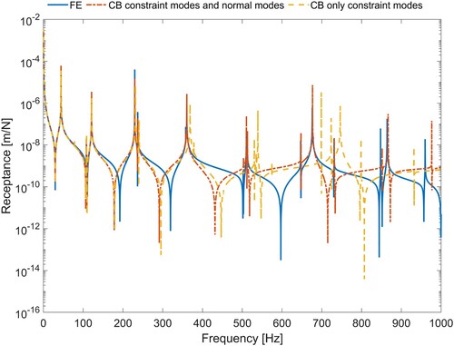7) The effect of the CB reduction as well as the simplification of only considering the constraint modes is studied by evaluating the point receptance of the undamped crossing rail model suspended with very soft springs. Three different modelling methods are compared: the full FE model, a CB reduction containing constraint modes and all normal modes up to 5000 Hz, and the adopted CB reduction where only the constraint modes are considered, see Figure 2. It is observed that the two reduced models are in good agreement up to ∼350 Hz but diverge as the frequency increases. Furthermore, it is argued that the reduced constraint mode model shows an agreement with the resonance peaks of the FE model that is considered sufficient for the intended frequency range (up to 500 Hz).

Figure 2. Point receptance at the crossing nose for three different model versions.

2.4. Retained nodes

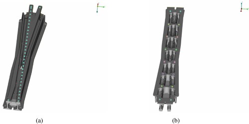
As indicated above, the crossing panel is assembled in a modular way after the rails have been generated in 13 separate pieces. This makes it easy to use different retained node discretisations for the different rails in the crossing panel. As the normal modes are neglected in the MBS model, the number and placement of the retained nodes are crucial to receive accurate results. Hence, the constraint modes alone are required to provide an accurate dynamic representation of the system. In addition to this, a sufficient retained node discretisation is important in Simpack as the wheel–rail contact and support forces are distributed and transferred through the retained nodes only. Retained nodes for the 3D crossing rail model are placed with a 15-cm interval (staying consistent with the discretisation used for the alternative beam element model of the crossing rail) in a straight line along the through route at nominal top of rail. These are connected to the nodes placed at the corresponding longitudinal positions on the running surface of the crossing rail using the Abaqus [18] keyword *Coupling in conjunction with the *Distributing option. Two retained nodes are also placed on the bottom of the crossing rail model at each rail fastening connection, while for all other rails only one node every 60 cm is used. Based on the crossing nose point receptance evaluated for different discretisations of the crossing rail, it was concluded that the present discretisation is sufficient (Figure 3).

Figure 3. (a) Retained nodes on the running surface of the crossing rail. (b) Retained nodes for the rail–sleeper fastenings on the bottom surface of the crossing rail. Between the positions for each sleeper, two longitudinal ribs reinforcing the reduced cross sections of the rail can be seen.

All dofs are retained for each retained node on the crossing rail, i.e. displacements in longitudinal (x), lateral (y) and vertical (z) directions. For the stock rails and sleepers, the FE beam model, retained node discretisation, retained and constrained dofs and the material parameters are taken from [2] except for the nodes connecting stock rail and crossing rail where rotations around y and z are also retained.

3. Procedure for model calibration

The model is calibrated for a measured locomotive run in the through route at 120 km/h. A novel approach for the calibration of the simulation model is presented. It uses Latin hypercube samples to explore the parameter space in a sensitivity analysis before a parameter optimisation is performed using a gradient-based method on a response surface built from a polyharmonic spline.

3.1. Sensor outputs

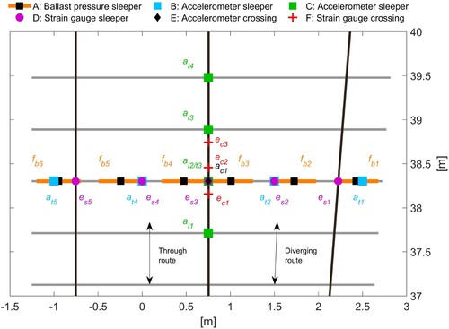
The crossing panel instrumentation that is used for the validation and calibration of the model is presented in Figure 4. The sensors used in the calibration process are divided into groups A–F. Sensors in group A are sleeper–ballast contact pressure sensors placed between sleeper and under sleeper pad [20]. Groups B, C and D are all placed on a sleeper, where B and C are accelerometers and D strain gauges. Groups E and F are placed on the bottom of the crossing rail, where E is a single accelerometer and group F consists of strain gauges. The sampling frequency of the strain gauges and accelerometers is 2.4 kHz, while the sleeper–ballast contact pressure sensors use a sampling frequency of 100 Hz. The acceleration signals from the instrumented demonstrator are reconstructed to displacements using the method developed in [15].

Figure 4. Sensor groups, locations and labels in the instrumented crossing panel.

To compare the response of the simulation model with the measurement data, signals from the simulation model corresponding with the sensors in the measurement setup need to be calculated. Based on the nodal displacements that are directly available as outputs from the simulation, the sleeper–ballast contact pressures, sleeper bending moments and corresponding strains are calculated using the methods presented in [2]. A new approach for determining the strain in the crossing rail is presented below.

3.2. Strain

To enable comparison between sensor and simulation results, the strain must be calculated for a position that corresponds to the placement of the relevant sensor. This is straightforward if the position corresponds to one that may be described by the retained nodes in the model reduction. If this is not the case, the displacements of the retained dofs ${\mathit{\rho }}^{\mathrm{R}}$ need to be transformed into the displacement vector $\mathit{u}$ of the original system using the transformation matrix $\mathit{T}$, see Equation  (6(6) $\mathit{u}=\left[\begin{array}{c}{\mathit{u}}^{\mathrm{R}}\\ {\mathit{u}}^{\mathrm{I}}\end{array}\right]=\left[\begin{array}{c}\mathit{I}\\ {\mathbf{\Phi }}^{\mathrm{C}}\end{array}\right]{\mathit{\rho }}^{\mathrm{R}}={\mathit{T}}_{\mathrm{C}}{\mathit{\rho }}^{\mathrm{R}}.$(6) ). When the displacement field has been acquired, the engineering strain between two points representing sensor j with the initial longitudinal length $L_j$, and the deformed longitudinal length $L_j+u_j$, can be approximated as (8) ${ϵ}_j=\frac{L_j+u_j}{L_j}.$(8)

3.3. Stress

The calculated displacements ${\mathit{\rho }}^{\mathrm{R}}$ from the MBS are transformed to the original FE discretisation (the discretisation used when generating the substructure) for a time step t using Equation  (6(6) $\mathit{u}=\left[\begin{array}{c}{\mathit{u}}^{\mathrm{R}}\\ {\mathit{u}}^{\mathrm{I}}\end{array}\right]=\left[\begin{array}{c}\mathit{I}\\ {\mathbf{\Phi }}^{\mathrm{C}}\end{array}\right]{\mathit{\rho }}^{\mathrm{R}}={\mathit{T}}_{\mathrm{C}}{\mathit{\rho }}^{\mathrm{R}}.$(6) ). This vector is denoted ${\mathit{u}}_{\mathit{t}}$. For each time step in the simulation, ${\mathit{u}}_{\mathit{t}}$ is assembled in a matrix $\mathit{U}$ containing $N_t$ (number of time steps) rows and $N_n$ (number of dofs) columns relating to the displacements of the full FE model, see Equations (9(9) $\begin{array}{rl}{\mathit{u}}_{\mathit{t}}& =\left[\begin{array}{cccc}{u}_{t,1}& u_{t,2}& \dots & u_{t,N_n}\end{array}\right]\end{array}$(9) ) and (10(10) $\begin{array}{rl}\mathit{U}& =\left[\begin{array}{cccc}{u}_{1,1}& u_{1,2}& \dots & u_{1,N_n}\\ u_{2,1}& u_{2,2}& \dots & u_{2,N_n}\\ ⋮& ⋮& \ddots & ⋮\\ u_{N_t,1}& u_{N_t,2}& \dots & u_{N_t,N_n}\end{array}\right]\end{array}$(10) ). Once $\mathit{U}$ is assembled, it can be used to impose prescribed displacements on all dofs for any time step. (9) $\begin{array}{rl}{\mathit{u}}_{\mathit{t}}& =\left[\begin{array}{cccc}{u}_{t,1}& u_{t,2}& \dots & u_{t,N_n}\end{array}\right]\end{array}$(9) (10) $\begin{array}{rl}\mathit{U}& =\left[\begin{array}{cccc}{u}_{1,1}& u_{1,2}& \dots & u_{1,N_n}\\ u_{2,1}& u_{2,2}& \dots & u_{2,N_n}\\ ⋮& ⋮& \ddots & ⋮\\ u_{N_t,1}& u_{N_t,2}& \dots & u_{N_t,N_n}\end{array}\right]\end{array}$(10) Based on the prescribed displacement field ${\mathit{u}}_{\mathit{t}}$, the finite element problem is statically solved in Abaqus for each time step t to obtain the time history of the stress field. When applying this method, local stresses can be easily determined from the global stress field at any given point in time. This approach will be demonstrated in Chapter 5 by evaluating the bending stresses of the ribs used on the bottom surface of the crossing casting, cf. Figure 3 (b). The ribs are sensitive to bending fatigue due to their reduced cross-section. This method is, however, costly in terms of computational time and is not included in the objective function for the calibration.

3.4. Model parameterisation

As described in Section 2.1, the stiffnesses of ballast and rail fastenings are parameterised in the model. The ballast is parameterised using six local parameters for gaps ($g_p$, $p=1,2,\dots ,6$) under the sleeper below the crossing nose and one uniform ballast stiffness scaling parameter for the entire track model ($h_1$). This results in the possibility of non-linear support stiffness for the crossing nose sleeper but assumes a linear support stiffness for all the other sleepers. The rail fastening stiffness is parameterised by a stiffness scaling parameter ($h_2$). The distribution of the gap (void) along the sleeper is linearly interpolated from the six parameters $g_p$.

3.5. Objective function

The simulation model is evaluated by comparing measured and simulated signals using an objective function based on the root mean square (RMS) value of the difference between the signals at each measurement point. This value is normalised by the RMS of the sum of the measured signals in each sensor group. To illustrate, let ${\overline{s}}_g$ be the sum of signals $s_{\mathrm{gk}}$ in the sensor group g with $N_g$ sensors. The contribution to the objective function from one sensor k in sensor group g can then be calculated as (11) $p_{\mathrm{gk}}=\frac{\mathrm{rms}(s_{\mathrm{gk},\mathrm{mea}}-s_{\mathrm{gk},\mathrm{sim}})}{\mathrm{rms}\left({\overline{s}}_{g,\mathrm{mea}}\right)},$(11) where sim and mea correspond to simulation and measurement, respectively. The objective function P quantifying the total quality of the fit is computed as (12) $P=\sum _{g=\mathrm{A}}^{g=\mathrm{F}}\sum _{k=1}^{N_g}{W}_g{p}_{\mathrm{gk},}$(12) where $W_g$ is a weighting factor for sensor group g. Initially, all weighting factors were set to 1, but for the final calibration $W_{\mathrm{C}}$ was increased to 3. To enable comparison, the compared signals were shifted in time and interpolated to have the same time discretisation.

3.6. Sensitivity study

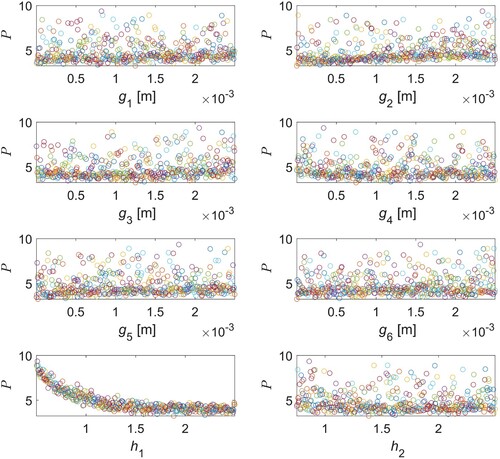
In the first step of the calibration procedure, a batch of 500 parameter sets is generated using the same initial parameter intervals as in [2]. To ensure that the entire parameter space is represented in the parameter samples, while keeping the amount of sets as low as possible, Latin hypercube sampling (LHS) [21] is used. Each parameter set is simulated in Simpack. Based on the results, a sensitivity study of the model is carried out and the influence of each parameter on the global (or an individual sensor's) objective function P can be examined. An example of the former can be seen in the scatter plots in Figure 5, where the results from all the LHS simulation runs are presented. Here the influence of each parameter on the objective function is presented. While it is clear that $h_1$ is the dominating parameter for the global objective function, the curve appears to flatten out for increasing $h_1$. As most of the sensors lie on the instrumented sleeper, their signals are heavily affected by both the sleeper–ballast gaps and the rail fastening and ballast stiffnesses (i.e. all unknown parameters). For sensors outside of the instrumented sleeper, the response relies heavily on the two latter.

Figure 5. Influence of the setting of each parameter on the global objective function.

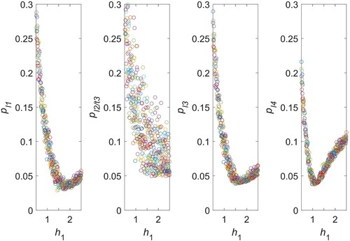
When studying individual sensor objective functions in sensor group C, a local minimum is seen for sensors which lie outside of the instrumented sleeper, see Figure 6, sensors $l1$, $l3$ and $l4$. This means that a further increase of ballast stiffness beyond the local minimum would strictly deteriorate the objective function for these sensors. On the other hand, this behaviour is not seen as clearly for the sensors on the instrumented sleeper, since a larger sleeper–ballast gap can be selected to compensate for a high ballast stiffness, see Figure 6, sensor l2/t3. As the effect from this behaviour on the global objective function is low, the initial calibration resulted in a very high ballast stiffness scaling parameter $h_1$. This motivated the increase in weight for the sensors in group C mentioned in Section 3.5.

Figure 6. Influence of the setting of $h_1$ on each individual objective function for sensors in group C. See placements of sensors in Figure 4.

Based on the sensitivity study, the parameter intervals are reduced and 500 new sets are generated. Again, the reduced parameter intervals are presented in [2]. In addition, 256 sets are generated covering all boundary combinations of the parameters. This is done to increase the accuracy of the response surface near the boundaries of the parameter interval. As for the first step of the calibration, all of the LHS generated parameter sets are simulated. The results are then used to calculate the objective function and to generate a response surface, see Section 3.7.

3.7. Response surface

The response surface is a polyharmonic spline, which is a linear combination of polyharmonic radial basis functions efficient for curve fitting and interpolation in any number of dimensions [22]. A general expression for a radial basis function is $\phi \left(\mathit{r}\right)$, where $\mathit{r}=\Vert \mathit{x}\Vert$ and $\Vert \cdot \Vert$ is the Euclidean distance function. Here, a polyharmonic radial basis function is defined as (13) $\begin{array}{ll}\phi \left(\mathit{r}\right)={\mathit{r}}^q& \mathrm{for}q=1,3,5,\dots \\ \phi \left(\mathit{r}\right)={\mathit{r}}^q\ln \left(\mathit{r}\right)& \mathrm{for}q=2,4,6,\dots \end{array}$(13) In this paper, a polyharmonic spline of order 3 is used, which is expressed as (14) $\hat{P}\left(\mathit{r}\right)=\sum _{j=1}^{N_d}\phi \left(\mathit{r}\right)w_j=\sum _{j=1}^{N_d}{\mathit{r}}^3{w}_j,$(14)

where $N_{\mathrm{d}}$ is the size of the training data vector used to generate the spline and $\mathit{r}=(\Vert \mathit{x}-{\mathit{c}}_{\mathit{j}}\Vert )$ is the Euclidean distance between the vectors $\mathit{x}$ and ${\mathit{c}}_{\mathit{j}}$. For the model calibration in this paper, $\mathit{x}$ is a vector containing n values, where n is the amount of calibration parameters (here, n = 8). The basis function centres $\mathit{c}$ are $N_d$ vectors containing n values, while $\mathbf{w}$ is a vector containing $N_d$ weighting factors. To generate the polyharmonic spline, the vector $\mathbf{w}$ must be determined. For this purpose, Equation (14(14) $\hat{P}\left(\mathit{r}\right)=\sum _{j=1}^{N_d}\phi \left(\mathit{r}\right)w_j=\sum _{j=1}^{N_d}{\mathit{r}}^3{w}_j,$(14) ) and the training data vector $\mathit{d}$ containing the objective function value $d_i$ for the parameter set ${\mathit{x}}_i$ are used to solve the following system of equations: (15) $\left[\begin{array}{cccc}\Vert {\mathit{x}}_1-{\mathit{c}}_1{\Vert }^3& \Vert {\mathit{x}}_1-{\mathit{c}}_2{\Vert }^3& \dots & \Vert {\mathit{x}}_1-{\mathit{c}}_{N_d}{\Vert }^3\\ \Vert {\mathit{x}}_2-{\mathit{c}}_1{\Vert }^3& \Vert {\mathit{x}}_2-{\mathit{c}}_2{\Vert }^3& \dots & \Vert {\mathit{x}}_2-{\mathit{c}}_{N_d}{\Vert }^3\\ ⋮& ⋮& \ddots & ⋮\\ \Vert {\mathit{x}}_{N_d}-{\mathit{c}}_1{\Vert }^3& \Vert {\mathit{x}}_{N_d}-{\mathit{c}}_2{\Vert }^3& \dots & \Vert {\mathit{x}}_{N_d}-{\mathit{c}}_{N_d}{\Vert }^3\end{array}\right]\left[\begin{array}{c}{w}_1\\ w_2\\ ⋮\\ w_{N_d}\end{array}\right]=\left[\begin{array}{c}{d}_1\\ d_2\\ ⋮\\ d_{N_d}\end{array}\right]$(15) When the weights have been determined, the response surface of the objective function can be formed and used in the calibration. In addition, the shape of the response surface can be examined to understand the sensitivity of each parameter.

3.8. Response surface validation

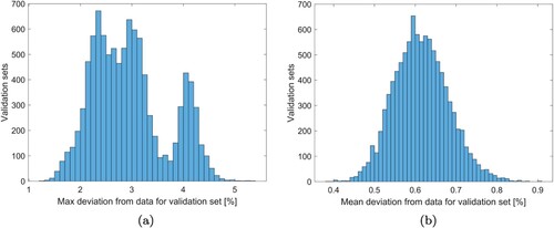
The polyharmonic spline is evaluated with Monte Carlo validation. This is done by randomly removing 75 samples from the data vector and adding them to a validation set. The spline is then generated using the calibration set, i.e. with the remaining 701 data samples. The maximum and mean percentage differences between the generated polyharmonic spline and the validation set are then calculated. This process is repeated 10,000 times to account for the statistical insecurity of the method. The results can be seen in Figures 7(a) and (b), showing a maximum deviation below 5.5% and a mean deviation below 0.9 %.

Figure 7. (a) Maximum deviation in the Monte Carlo validation. (b) Mean deviation in the Monte Carlo validation. Total number of validation sets = 10,000.

3.9. Calibration

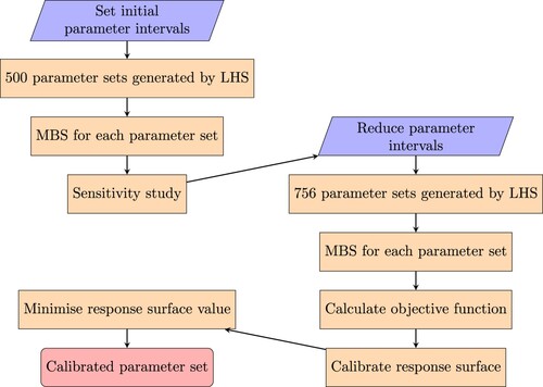
After the validation of the response surface, the calibration is performed by applying a gradient-based optimisation method using fmincon in Matlab R2021 [23]. It uses the interior-point algorithm to find the parameter set generating the minimum of the response surface. To ensure that the global minimum is found, 1000 start points are generated using LHS and running the optimisation algorithm from each start point. The entire calibration process is summarised in the flowchart in Figure 8.

Figure 8. Calibration flowchart.

4. Calibrated model

The calibrated parameter set is visualised in Figure 9. In Figure 9(a), the response surface of the objective function is plotted against the scaling factors of ballast stiffness and rail fastening stiffness around the found minimum. For this set of measured data, the calibrated bed modulus of the ballast is 120.7 (kN/mm)/m${}^2$ ($h_1\approx 1.81$) and the calibrated fastening stiffness is 29.4 kN/mm ($h_2\approx 1.18$). 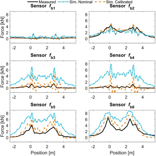In Figure 9(b), the calibrated distribution of sleeper–ballast gaps can be seen. The distribution shows voids especially underneath the crossing rail. The most significant improvement between the nominal and calibrated models can be seen for the sleeper–ballast contact forces in Figure 10, where the nominal model shows significant deviations from the measurement data, especially for sensors ${\mathrm{f}}_{b3}$ and ${\mathrm{f}}_{b4}$ near the crossing rail. The optimisation of the calibration problem was found to be practically convex. The solutions found were two almost identical parameter setups, with slight differences in the response surface value.

Figure 9. (a) Response surface of objective function plotted against scaling parameters for ballast stiffness $h_1$ and rail fastening stiffness $h_2$. (b) Ballast gap distribution for the calibrated model.

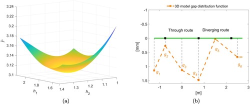
Figure 10. Time histories of sleeper–ballast contact force for group A sensors. Nominal and calibrated 3D models are compared with measured data.

5. Discussion and model comparison

To evaluate the difference between the 3D model developed in this paper and the alternative beam model presented in [2], the nominal versions of the two models are compared by plotting sensor responses from the measurements and simulations. The nominal models were chosen such that the influence from any differences in the calibration would not affect the comparison of the models. For most signals, the difference in simulated sensor outputs between the two models is very low. For example, the crossing strains from both models are plotted in Figure 11. For sensor group C in Figure 12, some differences can be seen primarily for the sensors ${\mathrm{a}}_{l1}$, ${\mathrm{a}}_{l3}$ and ${\mathrm{a}}_{l4}$. 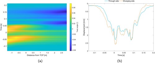This difference is mainly due to the twisting of the crossing rail and the improved model of the rail fastening in the 3D model. The further away from the crossing nose a sensor is placed, the further away it is from the rotation centre of the crossing rail leading to that the influence of the crossing rail twist on the sleeper displacement increases. For different longitudinal positions relative to the theoretical crossing point (TCP), the simulated time history of the twisting angle of the crossing rail is illustrated in Figure 13(a). It can be seen that when the leading wheelset of the bogie is approaching the crossing transition, the crossing rail twists towards the diverging route (see Figure 1) due to the lateral offset in the loading. As the bogie transitions across the crossing rail, the rotation of the crossing rail gradually changes direction towards the through route (see Figure 1). During the impact of the leading wheelset, the displacement of the crossing rail at the sleeper below the crossing nose is substantially affected by this twisting motion, see Figure 13(b).

Figure 11. Group F results for beam and 3D models with nominal parameter settings, and comparison with measured data.

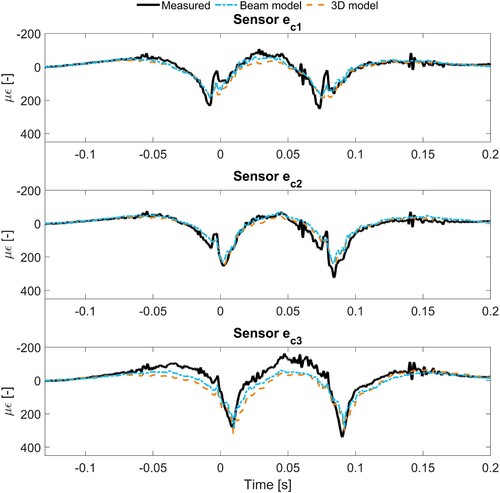
Figure 12. Group C results for beam and 3D models with nominal parameter settings, and comparison with measured data.

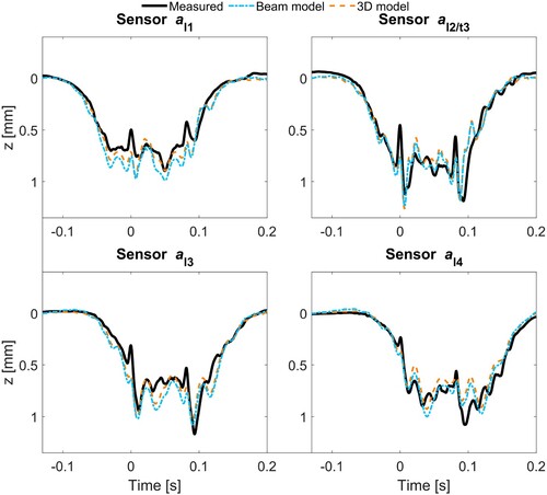
Figure 13. (a) Time history of crossing rail twist angle evaluated with the 3D model for positions along the crossing panel (relative to the distance from the TCP). (b) Displacements for the two crossing rail nodes that are used for the rail fastening to the sleeper under the crossing nose. See Figure 1 for diverging and through sides.

By modelling the rail fastening as two bushing elements connected to the sleeper instead of by one element, the bending moment distribution of the sleeper is shifted for some lateral positions. The effect of this shift in bending moment can be seen in the sleeper strains, mainly for sensor ${\mathrm{e}}_{s2}$ plotted in Figure 14. This results in an overall reduction of sleeper strain for this sensor and an improved agreement to measurement data.

Figure 14. Bending strain of sensor ${\mathrm{e}}_{s2}$ for beam and 3D models with nominal parameter settings, and comparison with measured data.

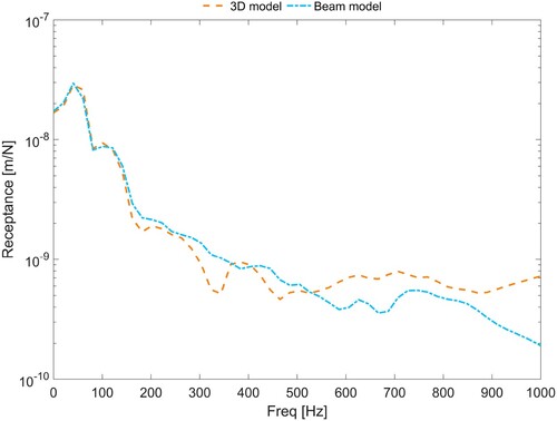
For a force excitation applied on the crossing nose, the point receptance of the two models with nominal parameter settings is compared in Figure 15. Very good agreement between the receptances is observed below 250 Hz. For higher frequencies, the receptances of the two models diverge. This indicates that the 3D model is needed to capture high-frequency behaviour of the crossing nose more accurately.

Figure 15. Point receptance at the crossing nose.

As the MBS model utilises substructures based on the Craig–Bampton method, the number of dofs for the 3D model can be kept low. In the present study, the increase in number of dofs is only 106 when using the 3D model instead of the beam model, changing from 798 to 904. However, the CPU time for the static equilibrium and subsequent time integration is increased from 30 to 40 minutes. Since the properties used for all the rail and sleeper bodies are independent of the parameterisation applied in this paper, the same set of substructures can be used independent of parameter settings. Therefore substructure generation time has not been included in the reported CPU time. For a parameterisation where new substructures would have to be generated for each run, the CPU time for the 3D model would increase by an additional 10% compared to the beam model.

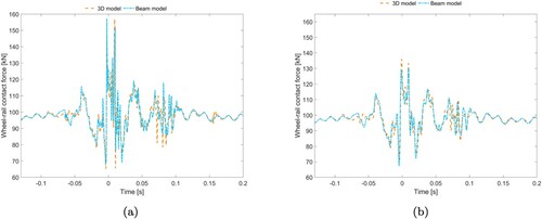
In Figure 16(a), the unfiltered vertical wheel–rail contact forces for the two models with nominal parameter settings can be seen. By low-pass filtering the wheel–rail contact forces, the influence of the difference in receptance at high frequencies seen in Figure 15 can be examined. As the receptances start diverging above 250 Hz, the wheel–rail contact forces in Figure 16(b) have been low-pass filtered at 250 Hz. It is concluded that the contribution to the contact force from frequencies exceeding 250 Hz is significant. However, by considering the low magnitudes of the crossing receptance for frequencies above 250 Hz, see Figure 15, it is argued that the influence of the high-frequency contribution on the structural deformation of the models is relatively low.

Figure 16. Time history of wheel–rail contact force for the leading wheel from the 3D and beam models: (a) no filter and (b) low-pass filtered at 250 Hz.

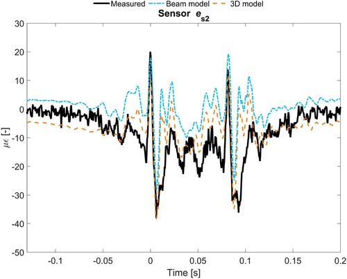
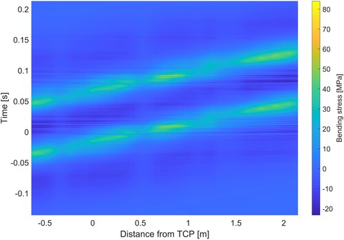
For the nominal 3D and beam models, time histories of the longitudinal bending stress along the most loaded rib on the bottom surface of the crossing rail are plotted in Figures 17 and 18, respectively. The three-dimensional stress state in the ribs was examined using the 3D model and was found to be close to uniaxial (longitudinal). The influence of the repetitive variation in rail cross-section on the bending stress can be clearly observed, as the sleeper fastening points where a solid cross-section is used show significantly lower stresses. As expected the maximum stress values are due to the impacts on the crossing nose occurring at around 0 seconds for the leading wheel and 0.08 seconds for the trailing wheel. For comparison, assuming uniaxial stress and using Hooke's law with the bending strains, the corresponding stresses have been calculated with the beam model [2]. The stresses of the two models show good qualitative agreement. However, quantitatively the beam model underestimates the bending stress in the reduced cross-section between two sleepers, while it overestimates the stress in the solid cross-sections above sleepers. For a static load case, the mesh used for the 3D model has been verified against a very fine mesh showing a discrepancy of maximum bending stress in the rib of 4 MPa.

Figure 17. Time history of longitudinal bending stress evaluated with the 3D model for positions along the crossing panel (relative to the distance from the TCP). The selected lateral coordinate on the crossing is aligned with the most loaded rib on the bottom surface of the crossing.

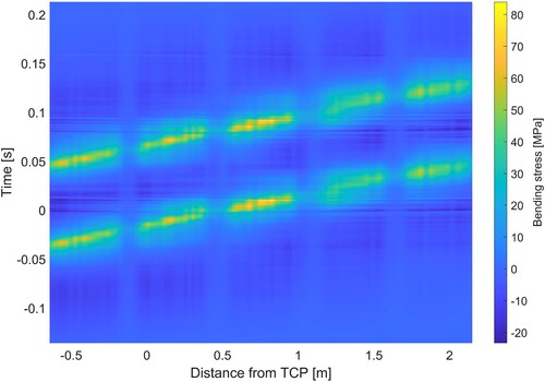
Figure 18. Time history of longitudinal bending stress evaluated with the beam model for positions along the crossing panel relative to the TCP.

6. Conclusion

A three-dimensional finite element model of a railway crossing panel for use in multibody simulations of dynamic vehicle–track interaction has been presented. The complete model is based on substructures generated from individual finite element models of the crossing rail, stock rails and sleepers. In particular, the crossing rail is generated from solid second-order elements to allow for an extensive evaluation of the distribution of stresses in the most loaded sections of the turnout in a post-processing step. The computational cost of running the model is relatively low facilitating optimisation of the crossing panel design.

The model was calibrated and validated to measured data from a comprehensively instrumented switch & crossing demonstrator installed in the Austrian railway network as a part of the European research programme Shift2Rail. A parameterisation with eight parameters relating to rail fastening and foundation stiffnesses and sleeper–ballast voids was introduced to enable the calibration. The presented calibration method uses Latin hypercube samples to explore the parameter space in a sensitivity analysis before a parameter optimisation is performed using a gradient-based method on a response surface built from a polyharmonic spline. For comparison, the differences in responses between the presented model and a previously developed and calibrated crossing rail model based on beam elements have been assessed. From the results, the following conclusions are drawn:

• The approach to calibrate the unknown support conditions by using a response surface that has been fitted from simulation results shows accurate and practically convex results. In the present study, the calibration resulted in non-uniform ballast support conditions with especially poor support and voids below the crossing rail.

• The twist angle of the crossing rail (accounted for in the 3D model) can have a significant impact on the displacements of the crossing, especially for the leading wheel impact which occurs while the weight of the bogie is very unevenly distributed on the crossing rail. However due to the selected placements of the sensors in the field measurements, little effect could be seen when comparing simulated signals against field measurement data.

• For the studied speed of 120 km/h, the introduction of a 3D model of the crossing rail shows little effect on the calculated wheel–rail contact forces, although a significant influence can be seen on the point receptance of the crossing nose at frequencies above 250 Hz.

• The longitudinal bending stress in the ribs on the bottom surface of the crossing rail is underestimated when using beam theory compared to the results of the 3D model.

• The calibrated beam and 3D models can be used in an optimisation of the design for reduced structural loading of the crossing panel.

Disclosure statement

No potential conflict of interest was reported by the author(s).

Additional information

Funding

The current work is part of the activities within the Centre of Excellence CHARMEC (CHAlmers Railway MEChanics, www.chalmers.se/charmec). Parts of the study have been funded within the European Union's Horizon 2020 research and innovation programme in the Shift2Rail project In2Track3 under grant agreement no. 101012456.The computations were enabled by resources provided by the National Academic Infrastructure for Supercomputing in Sweden (NAISS) and the Swedish National Infrastructure for Computing (SNIC) at C3SE partially funded by the Swedish Research Council through grant agreements no. 2022-06725 and no. 2018-05973.

References

- Pålsson BA. A parameterized turnout model for simulation of dynamic vehicle–turnout interaction with an application to crossing geometry assessment. In: Klomp M, Bruzelius F, Nielsen J, et al., editors. Advances in dynamics of vehicles on roads and tracks IAVSD 2019 Cham: Springer; 2020. (Lecture Notes in Mechanical Engineering). doi: 10.1007/978-3-030-38077-9_41
- Pålsson BA, Vilhelmson H, Ossberger U, et al. Dynamic vehicle–track interaction and loading in a railway crossing panel – calibration of a structural track model to comprehensive field measurements. Veh Syst Dyn. 2024;1–27. doi: 10.1080/00423114.2024.2305289
- Chen J, Wang P, Xu J, et al. Simulation of vehicle-turnout coupled dynamics considering the flexibility of wheelsets and turnouts. Veh Syst Dyn. 2023;61(3):739–764. doi: 10.1080/00423114.2021.2014898
- Alfi S, Bruni S. Mathematical modelling of train-turnout interaction. Veh Syst Dyn. 2009;47(5):551–574. doi: 10.1080/00423110802245015
- Grossoni I, Bezin Y, Neves S. Optimisation of support stiffness at railway crossings. Veh Syst Dyn. 2017;56:1–25. doi: 10.1080/00423114.2017.1404617
- Kassa E, Nielsen JCO. Dynamic train-turnout interaction in an extended frequency range using a detailed model of track dynamics. J Sound Vib. 2009;320:893–914. doi: 10.1016/j.jsv.2008.08.028
- Torstensson P, Squicciarini G, Krüger M, et al. Wheel–rail impact loads and noise generated at railway crossings – influence of vehicle speed and crossing dip angle. J Sound Vib. 2019;456:119–136 doi: 10.1016/j.jsv.2019.04.034
- Pedro J. Modelling and enhancing track support through railway switches & crossings [PhD thesis]. University of Huddersfield, UK; 2020.
- Bruni S, Anastasopoulos I, Alfi S, et al. Effects of train impacts on urban turnouts: modelling and validation through measurements. J Sound Vib. 2009;324:666–689. doi: 10.1016/j.jsv.2009.02.016
- Xin L, Markine V, Shevtsov I. Analysis approach of turnout crossing performance by field measurements and finite element modeling. Proceedings of the 24th Symposium of the International Association for Vehicle System Dynamics (IAVSD 2015), 2015 Aug 17-21; Graz, Austria: Taylor & Francis; 2016. p. 1593–1600. doi: 10.1201/b21185-169
- Otorabad HA, Bezin Y, Grossoni I, et al. Finite element analysis of a crossing panel under dynamic moving load – effect of support conditions and implications on foot fatigue. Proc Inst Mech Eng F J Rail Rapid Transit. 2023;237(5):563–575. doi: 10.1177/09544097221128162
- Grossoni I, Le Pen LM, Jorge P, et al. The role of stiffness variation in switches and crossings: comparison of vehicle-track interaction models with field measurements. Proc Inst Mech Eng F J Rail Rapid Transit. 2020;234(10):1184–1197. doi: 10.1177/0954409719892146
- Milošević MD, Pålsson BA, Nissen A, et al. Condition monitoring of railway crossing geometry via measured and simulated track responses. Sensors. 2022;22(3):1012. https://www.mdpi.com/1424-8220/22/3/1012. doi: 10.3390/s22031012
- Iwnicki S. Manchester benchmarks for rail vehicle simulation. Veh Syst Dyn. 1998;30(3–4):295–313. doi: 10.1080/00423119808969454
- Milošević MD, Pålsson BA, Nissen A, et al. Reconstruction of sleeper displacements from measured accelerations for model-based condition monitoring of railway crossing panels. Mech Syst Signal Process. 2023;192:110225. doi: 10.1016/j.ymssp.2023.110225.
- CALIPRI C4X measurement device. Available from: https://www.nextsense-worldwide.com/en/; 2023.
- Liang Z, Lee G, Dargush G, et al. Structural damping: applications in seismic response modification. 1st ed. Boca Raton: CRC Press, Boca Raton, Florida, USA; 2012. doi: 10.1201/b11449.
- Dassault Systemes. Abaqus reference; 2023.
- Craig RR, Bampton MCC. Coupling of substructures for dynamic analyses. AIAA J. 1968;6(7):1313–1319. doi: 10.2514/3.4741
- Loy H, Kessler M, Augustine A, et al. Switches & crossings: defined elasticity for new turnout designs. Rail Eng Int. 2022;2022(1):1–8.
- Olsson A, Sandberg G, Dahlblom O. On Latin hypercube sampling for structural reliability analysis. Struct Saf. 2003;25(1):47–68. doi: 10.1016/S0167-4730(02)00039-5
- Fasshauer GE. Meshfree approximation methods with Matlab. River Edge, New Jersey, USA: World Scientific, River Edge, New Jersey, USA; 2007.
- The Mathworks Inc. Matlab r2021; 2021.