Experimental parameter identification of scalable white and grey box jounce bumper models for ride comfort simulation

Abstract

The design of a passenger car’s ride and handling goals requires an enormous amount of hardware and prototypes. To avoid time-consuming testing activities, one crucial trend is the virtualisation of suspension development. Another goal of the virtualisation is the determination of vehicle properties at an early stage of the development process. Highly accurate suspension models are required to transfer the full vehicle’s characteristics into simulation tools. Since the jounce bumper is an important component of the suspension system, modelling its functional behaviour is essential for virtualised chassis development. Therefore, two dynamic modelling approaches are derived and compared in this contribution. One approach is based on local linear model networks and thus can be seen as a grey box model. The other approach consists of white box rheological elements, which allow the physical interpretability of the model parameters. The comparison of the approaches is based on experimental parameter identification, which includes synthetic and real excitations recorded on representative roads. The advantages of the proposed approaches will be discussed in terms of their suitability for the virtual design of the driving behaviour.

KEYWORDS:

• Ride comfort simulation
• nonlinear system identification
• local linear model network
• jounce bumper modelling
• Dahl friction model

Introduction

According to the study [1], virtualisation is a key trend to reduce hardware prototypes. In the context of the virtual development of ride comfort, we deal with the modelling of the jounce bumper. There are high requirements on the model, as the jounce bumper acts in a broad frequency range. In this contribution, we focus on the ‘primary ride’, which is characterised by the vehicle body motion in the range of approx. 0–5 Hz and the ‘secondary ride’, which describes the oscillation of various vehicle masses (unsprung masses, engine mass) in the range of approx. 5–25 Hz [2,3]. Especially the resonance frequencies of the chassis and the wheel cause high suspension travel and therefore a major impact of the jounce bumper on the ride comfort. In terms of jounce modelling, there are publications based on FEA methods. Wang et al. [4] designed a stratification method for polyurethane jounce bumpers consisting of three layers with different material properties. This model simulates the deformed shapes of the jounce and predicts the load–displacement–characteristic for small to medium strains (0–0.4) but yields errors at large displacements. To design the vehicle handling dynamics at an early stage of the development process, simplified approaches exist that use analytic functions to describe the load–displacement–characteristic [5]. As those approaches do not cover dynamic operating areas, they are not suitable for a simulative evaluation of ride comfort. Therefore, the goal of this contribution is to derive functional models for the jounce bumper, which capture the dynamic behaviour of a broad frequency range accurately. In addition, we focus on real-time capability and a parameterisation process requiring low measurement effort. To validate the models for ride comfort simulation, we use real excitation profiles recorded by full vehicle measurements.

The contribution is structured as follows: first, the influence of the jounce bumper on a vehicle’s ride and handling goals is explained briefly. Then, full vehicle measurements are analysed to quantify the operating area of the jounce bumper. Based on these results, a generic component measurement procedure is derived that covers a wide operating range. Afterwards, the measurement results for training and validation of the models are presented. This will be followed by a detailed explanation of the two modelling approaches and the experimental parameter identification methods.

Subsequently, the modelling results are presented, followed by a discussion of the approaches. Finally, a summary is given, and further tasks will be discussed.

Influence of the jounce bumper on vehicle ride and handling

To limit the suspension travel in the compression direction, there exist pressure stops (German: ‘Druckanschlag’) and jounce bumpers (German: ‘Zusatzfeder’). Pressure stops are typically made of elastomers and are very stiff and flat, allowing low design flexibility for the suspension travel characteristic [6]. The jounce bumper, which is covered in this contribution, is significantly taller than a pressure stop and is usually made of elastomer or polyurethan (PUR). For small jounce travel the stiffness is low but provides a progressive characteristic [7]. The jounce is located on the top-mount and is compressed by the damper housing. Depending on the top-mount concept, the jounce transfers its reaction force directly or via the top-mount stiffness into the chassis. Because of its progressive force-displacement-characteristic, the jounce protects the damper housing from hitting into the top-mount for impulse road disturbances like speed bumps or potholes. The jounce is not only essential for component protection but also for adjusting the handling and comfort properties of a vehicle in terms of functional development. For good ride comfort, both the chassis travel and the chassis acceleration should be kept low by the suspension system [8], which leads to a conflict of objectives. While short jounce bumpers isolate the chassis for small suspension travel, they lead to high chassis acceleration for high suspension travel and vice versa. In the application process of the jounce bumper, both static and dynamic properties are taken into account [9]. Furthermore, the jounce is required for designing the rolling behaviour of the vehicle at high lateral accelerations or contrary excitations through the road. Because of its ability to increase the tire normal force difference, the jounce also influences the steering behaviour.

Measurement methodology

In this chapter, we describe the process of measuring the operating area of the jounce bumper in the full vehicle and the transfer of those excitations to the component test bench. The relevant manoeuvres are determined in the context of ride comfort as a reaction to road surface irregularities, which can be seen as the major excitations of vehicle body oscillations [10].

Full vehicle operating ranges

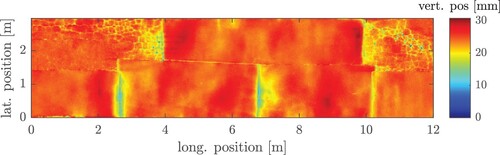
Full vehicle measurements were conducted to obtain the operating ranges of the jounce bumper in terms of displacement and displacement velocity. Since we focus on road-induced ride comfort, the measurements were carried out on roads (called road a–d) that have surface irregularities and are therefore suitable for a chassis suspension application. To cover a range of customer-relevant use cases, the driving velocity was chosen between 80 and 150 km/h, while the vehicle was occupied by three people (two in the front and one in the back). The manoeuvres include several phenomena, from small-amplitude excitations to transient events that cause high-suspension travel. For classification purposes, the road surfaces are scanned using a dGPS-system with a grid size of 5 mm. For details on road surface measurements, see Ref. [11]. As the 3D scan of a section of road a shows (Figure 1), there exist several road cracks and irregularities.

Figure 1. 3D surface scan of an exemplary road used for determining the operating areas of road-induced ride comfort.

In the following, the roughness of the scanned road profiles is characterised according to ISO 8608 [12], which is a classification standard for road surfaces. According to this method, the power spectral density (PSD) of the road unevenness $G_d(n)$ can be approximated by the equation (1) $\begin{array}{r}{G}_d(n)=G_d(n_0)\cdot {\left(\frac{n}{n_0}\right)}^{-w},\end{array}$(1) where $n$ $[1/\text{m}]$ denotes the spatial frequency and $w$ [−] describes the ‘waviness’. This characterises how the energy content of the unevenness is distributed among the frequency band. $G_d(n_0)$ [${\text{m}}^3$] denotes the power spectral unevenness density at the ‘reference spatial frequency’ $n_0=0.1$ $1/\text{m}$. As the mean waviness $w=2$ is assumed for an average road, ISO [12] proposes the classification of road surfaces into eight classes (A–H) depending on the PSD at the reference spatial frequency $n_0$. The average German highway is characterised by $G_d(n_0)=1.6\cdot {10}^{-5}{\text{m}}^3$ [13] and belongs therefore to class A. Class C for example describes unpaved roads and damaged pavements, according to Ref. [14].

Figure 2 shows the power spectral unevenness density of the different roads according to a smoothing algorithm of ISO 8608, whereby a mean lateral position was used for the evaluation. The algorithm calculates the road unevenness at the reference spatial frequency $G_d(n_0)$ and the waviness $w$ via a least mean square method in the range of 0.011–2.83 $1/\text{m}$ [12]. According to the algorithm, the roads provide road unevenness from $9.6\cdot {10}^{-5}$ to $1.4\cdot {10}^{-4}{\text{m}}^3$ (Table 1) and can thus be categorised in road classes B–C. All investigated roads possess a waviness $w>2$, which means that their signal energy is concentrated in a lower frequency range compared to an average road, resulting in a steeper drop of spectral unevenness than the classification scheme of ISO 8608.

Figure 2. Road unevenness classification according to ISO 8608.

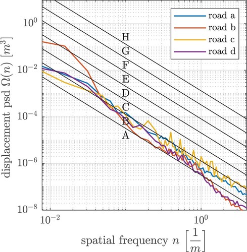
Table 1. Spectral unevenness density and waviness of the representative roads.

	Road a	Road b	Road c	Road d
$G_d(n_0)$ [${10}^{-6}$ ${\text{m}}^3$]	137	122	110	96
w	2.24	2.64	2.00	2.53

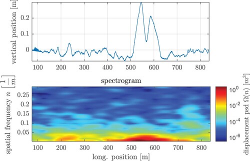
Classification of road profiles according to ISO 8608 is only recommended for roads with uniform statistical properties in terms of unevenness [15]. As the road b includes one pronounced bump to create a high suspension travel, an alternative approach is proposed to evaluate the road unevenness. While the PSD averages the oscillations of the underlying spectral frequencies with the loss of time information, the ‘spectrogram’ is a common way for signal analysis with respect to both frequency and time domain [16]. Figure 3 shows the spectrogram of the road unevenness of road b, whereas the signal mean at the spatial frequency 0 $1/\text{m}$ is not shown for visualisation purposes. The spectrogram is calculated with a Hann window of length 150 m (30,000 sample points with a grid size of 5 mm), whereby an amplitude correction was carried out to restore the signal energy content [17]. The bump, which is located in a longitudinal range of 510–630 m is characterised by a high energy content for spatial frequencies from 0 to 0.03 1/m. As this refers to a wavelength of approx. 35 m, the bump leads to a resonance for the chassis mass for driving velocities between 130 and 190 km/h, as the natural frequency of the sprung mass for ordinary passenger cars is usually in the range of 1–1.5 Hz [10].

Figure 3. Scanned road unevenness (above) and corresponding spectrogram (bottom).

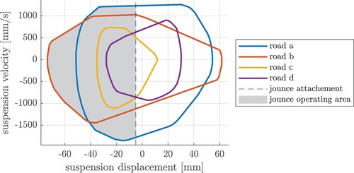
The vehicle was equipped with laser sensors (Figure 4) to record the suspension displacement, which is defined as the relative displacement between the damper housing and the chassis. Figure 5 shows the sign convention used for the following evaluations, i.e. a negative suspension displacement corresponds to a compression of the suspension system, while the jounce displacement is defined with a positive sign convention. Since the operating ranges are relevant in terms of displacement and displacement velocity, a phase portrait visualisation is suitable for the evaluation. Figure 6 shows the hull of the operating ranges on the different roads. Taking into account the attachment spacing of 5 mm, the operating range of the jounce bumper is given by the hatched grey area of the phase portrait. As it can be seen, the operating range is spanned by road a and road b, as road c and road d lie within the hulls of the other roads. While road a causes the highest displacement velocity up to 2000 mm/s, road b leads to the highest jounce displacement though the displacement velocity is lower. The maximum displacement trajectory of road b is due to the bump, which was characterised before by the spectrogram. This bump causes a resonance oscillation of the suspension system, leading to high suspension travel because the kinetic energy of the chassis must be stored by the suspension system. Figure 6 also shows that the absolute displacement velocity for the compression phase is higher than for the rebound phase. This is due to the damper characteristic, which provides lower damping forces for the compression direction than for the rebound direction to both isolate the chassis mass for bump excitations and dissipate the energy stored in the suspension after a transient excitation [18].

Figure 4. Road b for operating area measurement and laser sensor (blue) with reflecting screen (green) for recording suspension travel as well as hydropulse component test rig.

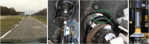
Figure 5. Visualisation of attachment spacing and definition of jounce travel and suspension travel (oriented to Ref. [6]).

Figure 6. Phase portrait of damper and jounce operating area.

Component test procedures

Based on the measured operating ranges of the jounce bumper, a component measurement procedure is designed, consisting of both synthetic and real excitations. As the operating area is spanned by road a and road b, these excitations are used to define the maximum displacement and displacement velocity of the measurement program and furthermore serve for validation of the models. The objective is to design a generic procedure for jounce bumpers that differ in characteristic properties like the unstressed length or the stiffness. Furthermore, operating ranges of heavily loaded vehicles should also be covered. Therefore, a safety margin of 10% is provided for the maximum displacement. While the maximum operating displacement $x_m=$ 68 mm on the real road causes a maximum jounce force of 3 kN, the safety margin leads to a maximum force of 9 kN, representing a safety margin of about 200%. In terms of potential energy stored in the jounce, the buffer leads to a safety margin of about 70% (Figure 7). To handle an arbitrary jounce bumper, the force–displacement–characteristic should be recorded first, whereas the displacement at 9 kN – called ‘reference displacement’ $x_{\text{ref}}$ – is used for scaling the measurement program.

Figure 7. Generalisation of the measurement program with safety margin.

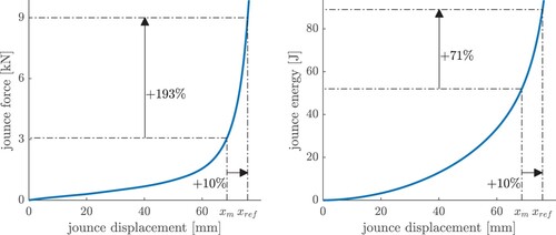
Table 2 shows the generic measurement procedure, consisting of synthetic and real excitations. The total measurement duration is about 15 min, while the excitation duration, involving only the excitation of the jounce, is significantly shorter for the dynamic profiles. For the amplitude sweep, a dwell time of 2 s is provided after every load to allow the relaxation of the jounce bumper, leading to a big difference between measurement duration and excitation duration. Figure 8 shows again the phase portrait of the operating area hull with respect to the jounce sign convention given in Figure 5. The synthetic excitations, which facilitate the model identification compared to the real excitations, cover the operating area recorded by the full vehicle measurements. For the amplitude sweep, the dynamic behaviour can be identified with constant frequency by sinusoidal half-waves and with constant velocities by dynamic ramps.

Figure 8. Synthetic excitations used for parameter identification.

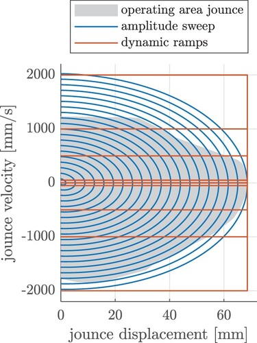
Table 2. Generic measurement procedure.

	Properties	Measurement goals	Measurement duration/ excitation duration [s]
Static ramps	Constant velocity (0.83 $\text{mm}/\text{s}$) Different turnaround points: $0.25\cdot x_{\text{ref}}$, $0.5\cdot x_{\text{ref}}$, $0.75\cdot x_{\text{ref}}$, $0.9\cdot x_{\text{ref}}$, $x_{\text{ref}}$	Force-displacement-characteristic Hysteresis shape for different turnaround points	510/420
Dynamic ramps	Constant turnaround point: $x_{\text{ref}}$ Different velocities: $25$, $50$, $500$, $1000$, $2000\text{mm/s}$	Dynamic response for constant velocities	80/22
Amplitude sweep	Linear increasing amplitude with constant frequency ($f[\text{Hz}]=\frac{2000[\text{mm/s}]}{2\pi \cdot x_{\text{ref}}[\text{mm}]}$)	Dynamic response for constant frequency	240/8
Road a	Real road excitation with safety margin	Real stimulation with focus on high displacement velocities	60/16
Road b	Real road excitation with safety margin	Real stimulation with focus on high suspension travel	20/7

Measurement results

In the following, the results of the jounce bumper measurements used for modelling and parameterisation are presented. Figure 9 shows the force–displacement–characteristic for the whole measurement procedure as a hull around all data points. As it can be seen, the jounce does not behave like a static nonlinear spring as there is a hysteresis area. A further evaluation of this specimen shows that the maximum hysteresis height is about 3 kN, occurring just below the reference displacement. The maximum hysteresis width is about 18 mm, occurring at a force of about 0.5 kN. Because of that, dynamic modelling elements must be considered for a proper virtualisation of the jounce behaviour.

Figure 9. Hull around force-displacement-characteristic of whole measurement procedure (left) and hysteresis shape (right).

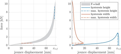
In the following, we will exemplarily show how the hysteresis is caused by the different excitations to get a better understanding of the jounce behaviour. Figure 10 (left) shows the static ramp excitations for the different turnaround points, while red denotes the compression phases and blue the rebound phases. As it can be seen, the static ramp excitations lie in the lower hysteresis area because there are no damping forces due to the low excitation velocity. The amplitude sweep is located in the upper area of the hysteresis, showing the ‘dynamic stiffening’ of the jounce bumper. It can also be seen that the hysteresis area for the amplitude sweep is slightly higher than for the static ramps. Thus, it can be stated that dynamic excitations increase both the jounce force and the hysteresis height.

Figure 10. Location of static ramps (left) and amplitude sweep (right) within the hysteresis of the whole measurement data.

Modelling approaches

Preprocessing and optimisation objectives

In this section, the jounce models as well as the optimisation-based parameterisation processes are presented. For calculating the jounce output force, both models require the jounce displacement and the velocity as input. As the velocity cannot be measured during the component test, it is extracted from the displacement signal as follows: first, the measured displacement is smoothed to suppress the measurement noise. This is done via a convolution of the recorded displacement signal and a Gauss-kernel. As this kernel represents a non-perfect impulse, this method can be seen as a low pass filter without phase shifting via a moving weighted average of the noised displacement signal. The intensity of the filtering can be adjusted by the standard deviation of the Gauss-kernel, whereby a high standard deviation leads to a high filtering and vice versa [19]. For the following investigations, a standard deviation of $0.005\text{s}$ was used to design the Gauss-kernel, which leads to a Gaussian-shaped transfer function with a standard deviation of 32 Hz in the frequency domain. Afterwards, the numerical differentiation of the smoothed displacement signal is implemented via a central finite difference method of order 4 [20].

The normalised root mean squared error (NRMSE) serves as an objective criterion to assess the modelling results. It is defined for a discretized measurement force $F_{\text{meas}}$ and a corresponding simulation signal $F_{\text{sim}}$ of dimension $N$ as follows: (2) $\begin{array}{r}\text{NRMSE}=\sqrt{\frac{{\sum }_{i=1}^N{(F_{\text{meas}}-F_{\text{sim}})}^2}{{\sum }_{i=1}^N(F_{\text{meas}}-\overline{F_{\text{meas}}}){}^2}}.\end{array}$(2)

Therefore, the NRMSE can be interpreted as the root mean square (RMS) value of the modelling error $F_{\text{meas}}-F_{\text{sim}}$ related to the standard deviation of the measurement data. The NRMSE is typically expressed as a percentage, whereas 0% represents a perfect fit and higher values are associated with poor model quality or noisy data. The NRMSE is only calculated for the excitation times (Table 2), while the overall cost function for the optimisation tasks is given by the mean NRMSE for the five excitation profiles.

White box model consisting of rheological elements

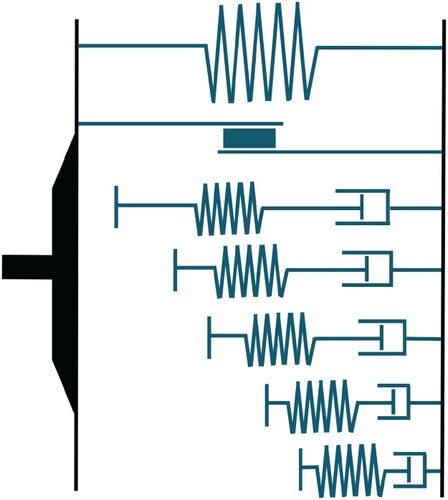
In this section, the white box model of the jounce as well as the underlying fitting process for the optimal parameterisation are explained. Figure 11 shows the topology of the model, which consists of parallel submodels. The total jounce force is modelled by a static nonlinear force–displacement–characteristic, a modified Dahl friction model and a subsystem consisting of five Maxwell elements with different contact points (free travel). Hence, as the displacement increases, more and more elements are excited and submit their individual reaction forces.

Figure 11. Topology of the white box model.

To ensure a robust parameterisation process, several model properties are identified directly from the measurement data. Nevertheless, several iterative optimisation routines based on time series are used. These direct and iterative methods derive a proper initialisation of a final fitting process that balances the parameters. In the following, the necessity of the different submodels is shown and the parameterisation algorithm is described by means of measurement data of a specific jounce bumper. The automation of the process for an arbitrary specimen with a focus on robustness is also explained.

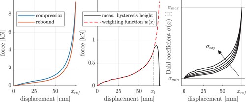
First, the static nonlinear force–displacement–characteristic $F_{\text{nl}}(x)$ and the modified Dahl model are identified based on the static ramp excitations. As the Maxwell elements act like dampers for small excitation frequencies, their impact on that kind of excitation is omitted because they do not transfer reaction forces. Figure 12 shows the compression (upper) and rebound (lower) characteristics of the jounce and the measured hysteresis height for the static ramp. As it can be seen, the hysteresis height increases monotonically up to a displacement of approx. 71 mm. Conventional hysteresis models like the Dahl model [21] represent constant (saturation) forces – with the exception of the transition phase after a change in the sign of the velocity. Thus, we modified the Dahl model with a displacement-dependent weighting function $w(x)$ for the output force. As Figure 12 also shows, the hysteresis height decreases just before the turning point of the excitation. This is caused by the transition phase of the rebound characteristic and can be modelled by the Dahl coefficient. As the transition phase in the rear part of the hysteresis depends on both the weighting function and the Dahl coefficient, this leads to an overdetermined modelling problem. Therefore, a weighting function is constructed for the overdetermined part in an intuitive way as follows: the hysteresis shows a similarity to the force–displacement–characteristic for displacements smaller than approx. 67 mm. Therefore, a continuation of this curve is plausible to complete the constructed weighting function $w(x)$. To automate this assumption, the displacement $x_1$ is defined as the transition of a left bend $\left(\frac{d^2{F}_{\text{hys}}}{d{x}^2}>0\right)$ to a right bend $\left(\frac{d^2{F}_{\text{hys}}}{d{x}^2}<0\right)$ of the hysteresis height. For a displacement, $x<x_1$ the weighting function is defined by the measured hysteresis height. For a displacement, $x_1<x<x_{\text{ref}}$ the weighting function is constructed by scaling and shifting of the force-displacement-characteristic. The scaling and shifting parameters are designed to ensure a C0- and C1-continuous transition between the measured hysteresis height and the constructed continuation at $x_1$. Note that this constructed hysteresis height could only be confirmed as the true hysteresis height by a static excitation of a sufficient high displacement that ensures a saturated output force of the Dahl model for the rebound phase.

Figure 12. Force-displacement-characteristic of static ramp (left), measured hysteresis height and constructed weighting function (middle), generic approach for displacement-$\sigma$-characteristic by three parameters (right).

In the following, the Dahl coefficient $\sigma$ is determined, whereby a displacement dependency is assumed as an extension of the conventional Dahl model. There is no intuitive choice for choosing polynomial approaches and even optimising the breakpoints of the $\sigma$-displacement-characteristic does not seem effective due to the high amount of optimisation parameters. Thus, the displacement dependency will be modelled by three functional scaling parameters, which enable the interpretability (Figure 12 right): while the Dahl coefficient should be ${\sigma }_{\text{min}}$ for $x=0$ and ${\sigma }_{\text{max}}$ for $x=x_{\text{ref}}$, the range in between is described by a distortable normalised weighting function using an exponent ${\sigma }_{\text{exp}}$ according to the following formula: (3) $\begin{array}{r}\sigma (x)={\sigma }_{\text{min}}+{\left(\frac{w(x)}{w(x_{\text{ref}})}\right)}^{{\sigma }_{\text{exp}}}\cdot ({\sigma }_{\text{max}}-{\sigma }_{\text{min}}).\end{array}$(3)

Figure 12 shows how these three parameters can represent a generic $\sigma$-displacement-characteristic. The differential equation for the Dahl model with displacement dependent $\sigma$ is given by (4) $\begin{array}{r}\frac{d{\tilde{F}}_{\text{Dahl}}(x,v,t)}{\mathrm{dt}}=\sigma (x)\cdot \left(1-\frac{{\tilde{F}}_{\text{Dahl}}(x,v,t)}{\frac{w(x_{\text{ref}})}{2}}\cdot \text{sign}(v)\right)\cdot v.\end{array}$(4)

As the hysteresis shape is defined by both the upper and the lower characteristics of the Dahl model, half of the constructed weighting function at the reference deflection $\frac{w(x_{\text{ref}})}{2}$ is used to limit the maximum force ${\tilde{F}}_{\text{Dahl}}(x,v,t)$, which is about 0.9 kN for this specimen.

The final output taking into account the weighting function is calculated by (5) $\begin{array}{r}{F}_{\text{Dahl}}(x,v,t)={\tilde{F}}_{\text{Dahl}}(x,v,t)\cdot \frac{w(x)}{w(x_{\text{ref}})}\end{array}$(5) to describe the hysteresis height accurately.

The static nonlinear force–displacement–characteristic $F_{\text{nl}}(x)$ can now be derived from the fact that the measured force $F_{\text{meas}}(t)$ for static excitations is equal to the sum of the nonlinear force–displacement–characteristic and the output force of the modified Dahl model: (6) $\begin{array}{r}{F}_{\text{meas}}(t)=F_{\text{nl}}(x)+F_{\text{Dahl}}(x,v,t).\end{array}$(6)

The remaining parameters ${\sigma }_{\text{max}}$, ${\sigma }_{\text{min}}$ and ${\sigma }_{\text{exp}}$ are then calculated by an optimisation problem. For that purpose, the static ramp excitations were conducted at different turnaround points to gain information about the displacement dependency of the transition phase. The optimisation algorithm defines the parameters depending on the error between the measured and the simulated force. Figure 13 shows the result of the fitting process for the Dahl model. On the left, the F-s-diagram of the Dahl model without the weighting function ${\tilde{F}}_{\text{Dahl}}$ is shown. The coefficient $\sigma (x)$ becomes higher with rising displacement, which causes steeper transition phases. On the right, the final Dahl output force $F_{\text{Dahl}}$ with the additional consideration of the identified weighting function shows the displacement dependency of the hysteresis width. Figure 14 shows that the static ramp measurement with the identified turnaround points can be modelled very accurately by the proposed submodels.

Figure 13. Dahl model output with displacement-dependent Dahl coefficient (left) and the additional weighting function (right) for static ramps with different turnaround points.

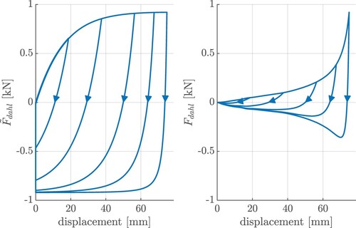
Figure 14. Comparison of measurement and model for the static ramps with different turnaround points.

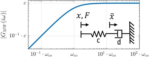
The second fitting routine focuses on dynamic excitations and parameterises the contact points, the stiffnesses and the cut-off frequencies of the Maxwell elements. As Figure 10 shows, the jounce responds with higher forces when the displacement velocity is increased. This effect is called dynamic stiffening and can be modelled by a Maxwell element (Figure 15), whose dynamic behaviour can be described in the time domain as (7) $\begin{array}{r}{F}_{\text{MW}}(t)=c\cdot (x(t)-\tilde{x}(t))=d\cdot \tilde{\dot{x}}(t),\end{array}$(7) whereas $\tilde{x}$ denotes the connection point between the spring and the damper.

Figure 15. Amplitude of the frequency response function of a generalised Maxwell element.

The transfer function of a Maxwell element $G_{\text{MW}}(s)$ can be derived by transferring Equation (7) in the Laplace domain, whereby $s$ denotes the Laplace variable: (8) $\begin{array}{r}{G}_{\text{MW}}(s)=\frac{F_{\text{MW}}(s)}{x(s)}=\frac{c\cdot s}{s+{\omega }_{\mathrm{co}}}.\end{array}$(8) The cut-off frequency ${\omega }_{\text{co}}$ is defined by ${\omega }_{\text{co}}=\frac{c}{d}$.

To interpret the dynamic behaviour of the Maxwell element, Figure 15 shows the amplitude of the frequency response function (FRF) given by $|G_{\text{MW}}(\mathrm{i\omega })|$. The Maxwell element acts like a spring for high frequencies but does not transfer any forces for low excitation frequencies. Therefore, it is suitable for modelling of the dynamic stiffening, while the low-frequency forces of the jounce can be covered by the model parts presented before. As the cut-off frequency defines the intersection of the asymptotes of the FRF, it can be parameterised for a suitable initial guess by the following consideration: ${\omega }_{\text{co}}$ must be higher than the excitation frequencies of the static ramp and lower than the excitation frequencies of the dynamic excitations.

In the following, we take a closer look at the dynamic stiffening force $F_{\mathrm{\Delta dyn}}$, which we define as the difference between the measured force $F_{\text{meas}}$ and the output force given by the nonlinear force–displacement–characteristic $F_{\text{nl}}(x)$ and the modified Dahl model $F_{\text{Dahl}}(x,v,t)$: (9) $\begin{array}{r}{F}_{\mathrm{\Delta dyn}}=F_{\text{meas}}-(F_{\text{nl}}(x)+F_{\text{Dahl}}(x,v,t)).\end{array}$(9)

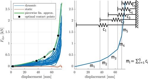
To get an impression of $F_{\Delta \text{dyn}}$, Figure 16 shows the dynamic stiffening force for both dynamic and static excitations in the F-s-diagram. $F_{\Delta \text{dyn}}$ is low for the static excitations, which means they are represented by the previous model parts quite well. This also justifies the omission of the Maxwell elements for the parameterisation of these model parts. For dynamic excitations, the specimen shows a dynamic stiffening force up to 2.8 kN for high displacements. As the dynamic stiffening seems to be nonlinear, we propose to model this by several Maxwell elements, which differ in their contact points (free travel). In that context, the upper enveloping of the F-s-diagram, which is caused by the highest velocities, can be used for a pre-estimation of the Maxwell stiffnesses by the following consideration: a single Maxwell element can be replaced by a spring for an infinite excitation velocity, which would result in a linear characteristic in the F-s-diagram. The nonlinear enveloping characteristic is now approximated by a piece-wise linear function via an optimisation problem. The optimal bending points can be interpreted as the contact points (free travel) of the springs and the gradients $m_i$ are equal to the sum of the stiffnesses which are in contact. Figure 16 shows, that the envelope can be represented quite well with five springs, thus five Maxwell elements are required. The stiffnesses pre-estimated in this way can be seen as a lower bound of the ‘true’ stiffnesses, as the excitation velocities are limited.

Figure 16. Pre-identification of Maxwell stiffnesses and contact points via a piece-wise linear approximation of the nonlinear hull.

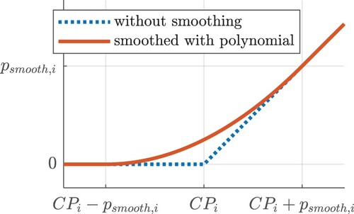
Because of these proper initial guesses, a local optimiser is used to parameterise the Maxwell elements based on the NRMSE of a time series representation. While this fitting routine parameterises the pre-estimated stiffnesses and cut-off frequencies, the contact points $\text{C}{\text{P}}_i$ are fixed. The time series data for this fitting process contains both static and dynamic excitations to guide the optimiser towards the optimal parameterisation. To shape a smooth fade-in of the Maxwell elements, an additional optimisation parameter $p_{\text{smooth}}$ is required that defines a transition phase around the contact point between $x=\text{C}{\text{P}}_i-p_{\text{smooth}}$ and $x=\text{C}{\text{P}}_i+p_{\text{smooth}}$ (Figure 17). To model a C0- and C1-continuous transition, a polynomial of order 3 is necessary because of the resulting four constraints.

Figure 17. Input smoothing around the contact point of a Maxwell element.

The output of the Maxwell elements is limited to compression forces as the jounce can only transfer forces in one direction. To attach the Maxwell elements to their optimal contact points, the states of the Maxwell elements are reset after each load event.

To simulate the output force of the Maxwell elements, the z-transform [22] is used to calculate the discrete output (sample time $T_s$) of the continuous transfer function given by Equation (8) via the bilinear transformation (10) $\begin{array}{r}s=\frac{2}{T_s}\cdot \frac{z-1}{z+1}.\end{array}$(10)

This leads to the discrete transfer function (11) $\begin{array}{r}G(z)=\frac{b_{\text{disk}}\cdot z-b_{\text{disk}}}{z+a_{\text{disk}}}=\frac{F(z)}{x(z)}\end{array}$(11) for a single Maxwell element, whereas the coefficients are given by (12) $\begin{array}{rl}{a}_{\text{disk}}& =\frac{{\omega }_{\text{co}}\cdot T_s-2}{{\omega }_{\text{co}}\cdot T_s+2},\end{array}$(12) (13) $\begin{array}{rl}{b}_{\text{disk}}& =\frac{2\cdot c}{{\omega }_{\text{co}}\cdot T_s+2}.\end{array}$(13)

Thus, the discrete output force can be calculated via $y(z)\cdot z^{-1}=y_{k-1}$ by (14) $\begin{array}{r}{F}_k=-a_{\text{disk}}\cdot F_{k-1}+b_{\text{disk}}\cdot (u_k-u_{k-1}),\end{array}$(14) whereas k denotes the discrete time step.

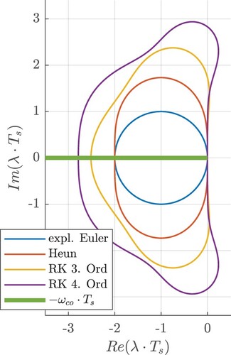
To ensure stability when simulating the differential equation with a numeric solver, the optimisation process is carried out with constraints for the maximum cut-off frequencies of the Maxwell elements.¹ As the pole of the transfer function given by Equation (8) is equal to the negative cut-off frequency and lies therefore on the negative real axis, the product $-{\omega }_{\text{co}}\cdot T_s$ has to lie in the stability regions of numeric solvers which are exemplarily shown in Figure 18 [23]. If, for example, stability should be guaranteed for a simulation sample time of $T_s=0.001\text{s}$, the maximum cut-off frequency must not be higher than $2000\text{rad/s}$. To ensure not only stability but also good accuracy, some buffer to the instability region can be provided.

Figure 18. Stability regions of numeric solvers and location of the product of the pole and the sample time for a generic Maxwell element.

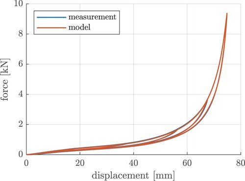
The third fitting routine is used to balance the pre-identified parameters. Therefore, there are no limitations on the shape of the training data, while the previously mentioned constraints for the Maxwell elements are still valid. The cost function is defined as the mean NRMSE for the five excitations of (Table 2). Figure 19 shows the result of the overall fitting process for exemplary excitations. The top two plots depict a static ramp excitation in the F-s-diagram and the F-t-diagram. While the Maxwell elements do not contribute an output force because of the low excitation velocity, the modified Dahl model and the static nonlinear force-displacement-characteristic can reproduce the measured force. For the dynamic ramp (bottom left), the Maxwell elements model the dynamic stiffening quite well, while the static characteristic would only cover the low-frequency force. The real excitation profile (bottom right) shows that comfort-relevant operating areas can be reproduced very accurately by the proposed white box model. The overall combined NRMSE after balancing the parameters is 3.86% (Table 3).

Figure 19. Exemplary comparison for quasi-static ramp excitation in F-s-diagram and F-t-diagram (top), dynamic ramp and real excitation (bottom).

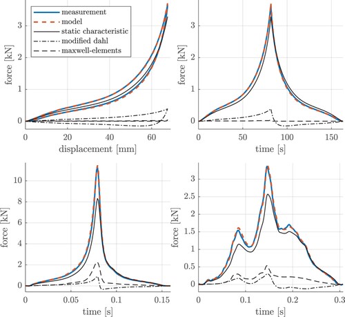
Table 3. White box model performance (NRMSE) for the several excitation profiles.

Excitation	NRMSE
Static ramps	1.77%
Dynamic ramps	4.36%
Amplitude sweep	2.39%
Road a	5.93%
Road b	4.86%
Combined	3.86%

Grey box model consisting of continuous local linear model network

In the following, a grey box model approach, applied as a generic force element based on [24], is presented to depict the specific dynamic behaviour of a jounce element. The fundamental concept is derived from Refs. [25] and [26] and was already applied to several modelling tasks like in Refs. [27] and [28]. Basically, in each time step k a set of i = [1,  … , M] discrete local linear models with p input variables $u$ of the form (15) $\begin{array}{r}{\hat{y}}_{i,k}=g_{i0}+\sum _{n=1}^{d_y}-a_{\mathrm{in}}\cdot y_{k-n}+\sum _{j=1}^p\sum _{n=0}^{d_{u,j}}{b}_{\mathrm{ijn}}\cdot u_{j,k-n}\end{array}$(15) is computed. Applying feedback of the overall model output y, which is calculated for the time step k by a weighted sum according to (16) $\begin{array}{r}{y}_k=\sum _{i=1}^M{\mathrm{\Phi }}_i(\mathit{z})\cdot {\hat{y}}_{i,k}\end{array}$(16) ensures an efficient computation of the coefficients by solving a least squares optimisation problem [25]. The weighting of each local model is here represented by a $n_z$-dimensional normalised Gaussian (17) $\begin{array}{r}{\mathrm{\Phi }}_i(\mathit{z})=\frac{{\mu }_i(\underset{\_}{z})}{{\sum }_{j=1}^M{\mu }_j(\underset{\_}{z})}\end{array}$(17) with (18) $\begin{array}{r}{\mu }_i(\mathit{z})=e^{\sqrt{{(\mathit{z}-{\mathit{c}}_i)}^T\cdot {\mathbf{\Sigma }}_i^{-1}\cdot (\mathit{z}-{\mathit{c}}_i)}},\end{array}$(18) where ${\mathit{c}}_i$ and ${\mathbf{\Sigma }}_i$ represent the centre vector and covariance matrix, respectively. The independent input variable $\mathit{z}$ consists of a selectable subset of [${\hat{y}}_{i,k},\dots ,{\hat{y}}_{i,k-d_y},u_{j,k},\dots ,u_{j,k-d_{u,j}}$]. In this contribution the covariance matrix is only of diagonal type to maintain the interpretability as a fuzzy system [25]. The partitioning of the operating ranges is determined by executing the local linear model tree (LoLiMoT) algorithm [29]. This methodology addresses drawbacks of fixed model structures by deploying an iterative refinement of the same.

Since in this context, the jounce force element is intended to be used basically in a continuous full vehicle simulation either for offline desktop applications or in an online real-time environment, a transition from discrete to continuous system definition is beneficial. It is always possible to identify the model parameters by taking numerical integration requirements into account, so that this subsystem can be solved in a stable and accurate manner. Nevertheless, this does not necessarily ensure a stable solution of the global system due to a change of its eigenvalues. This can be addressed by using a proper fixed-step or variable-step solver configuration to compute the entire stack of system equations. The drawback of an increased computational effort compared to using a discrete system, where the coefficients can directly be determined and thus no iterative nonlinear optimisation process is necessary, depends on the practical use case but can be neglected here due to only slightly increased computation time.

For the conversion to the continuous time domain, it is assumed that in Equation (15) the local model output $\hat{y}$ is fed back, which is approximately valid for the subspace of the operating range of that specific local model with the neglectable activity of the other remaining models. By applying the z-transform [22] on this modified Equation (15), the input-related numerator N and denominator D of the discrete transfer function can be written as (19) $\begin{array}{r}{N}_{\mathrm{ij}}(z)=\sum _{n=0}^{d_{u,j}}{b}_{\mathrm{ijn}}\cdot z^{-n}\end{array}$(19) and (20) $\begin{array}{r}{D}_i(z)=1+\sum _{n=1}^{d_y}-a_{\mathrm{in}}\cdot z^{-n}.\end{array}$(20)

After combining an artificial step input (Heaviside function) $H(z)$ with the constant offset, the difference equation can be stated as (21) $\begin{array}{r}{\hat{Y}}_i(z)=\frac{g_{i0}}{D_i(z)}\cdot H(z)+\sum _{j=1}^p\frac{N_{\mathrm{ij}}(z)}{D_i(z)}\cdot U_j(z)\end{array}$(21) and partially transferred to the Laplace domain by applying a bilinear transformation [22], which yields (22) $\begin{array}{r}{\hat{Y}}_i(s)\approx {\hat{Y}}_i(z){|}_{z=\frac{1+\frac{T}{2}s}{1-\frac{T}{2}s}}=G_{i0}(s)\cdot H(s)+\sum _{j=1}^p{G}_{\mathrm{ij}}(s)\cdot U_j(s).\end{array}$(22)

In order to reduce the system complexity, the dynamic behaviour of $G_{i0}(s)$ for reaching a constant offset in each local model is neglected and set to a fixed value by taking the linearity property of a Laplace transform into account and applying the final value theorem according to (23) $\begin{array}{r}{g}_{i0}(t=\mathrm{\infty })=\underset{s\to 0}{lim}s{G}_{i0}(s)\cdot \frac{1}{s}={\tilde{g}}_{i0}.\end{array}$(23)

Finally, this can be converted to the following time-invariant continuous state space representation in controllable canonical form [30] (24) $\begin{array}{rl}\dot{\mathit{x}}(t)& =\left[\begin{array}{ccc}{\mathbf{A}}_1& \cdots & 0\\ ⋮& \ddots & ⋮\\ 0& \cdots & {\mathbf{A}}_M\end{array}\right]\mathit{x}(t)+\left[\begin{array}{c}{\mathbf{B}}_1\\ ⋮\\ {\mathbf{B}}_M\end{array}\right]\mathit{u}(t)\end{array}$(24) (25) $\begin{array}{rl}\hat{\mathit{y}}(t)& ={\tilde{\mathit{g}}}_0+\left[\begin{array}{ccc}{\mathit{c}}_1^T& \cdots & 0\\ ⋮& \ddots & ⋮\\ 0& \cdots & {\mathit{c}}_M^T\end{array}\right]\mathit{x}(t)+\left[\begin{array}{c}{\mathit{d}}_1^T\\ ⋮\\ {\mathit{d}}_M^T\end{array}\right]\mathit{u}(t),\end{array}$(25) where the corresponding non-zero matrix coefficients are subsequently set as optimisation variables. The initial state of the system is derived by a least square minimisation of both the internal initial dynamics and the difference to a potential non-zero initial output value using the Penrose pseudo-inverse [31] as follows: (26) $\begin{array}{r}{\mathit{x}}_0={\left[\begin{array}{c}\mathbf{A}\\ \mathbf{C}\end{array}\right]}^{-1}\cdot \left(\left[\begin{array}{c}\mathbf{B}\\ \mathbf{D}\end{array}\right]\cdot {\mathit{u}}_0+\left[\begin{array}{c}0\\ {\mathit{g}}_0-{\mathit{\Phi }}_0^{-1}\cdot y_0\end{array}\right]\right)\end{array}$(26) During the parameter identification process the numeric integration is carried out by applying a triangle-hold discretization method as described in Ref. [22].

Applying the generic force element modelling concept described above to depict the dynamic system behaviour of a jounce requires the definition of proper input variables, system configuration (e.g. order and number of local models, selection of variables for input space partitioning), numerical limitations and a strategy for an efficient parameter identification process. Here, two system input variables were chosen by the jounce displacement as well as a representation of the nonlinear quasi-stationary characteristic depending on the displacement. Thus, the latter can be interpreted as a Hammerstein model [25]. In contrast to the white box modelling approach above this tabled characteristic is directly derived by computing the mean value of the hysteresis depicted in Figure 12 (left). For the sake of clarity, also no (modified) Dahl friction model is added in parallel to this grey box approach. Since this model is intended to run in an arbitrary full vehicle simulation environment, no delay will be applied to the variables used by the input space partitioning. Furthermore, the jounce displacement and the corresponding velocity of the current simulation step are chosen to calculate the activity level of each local linear model. A variation of input signals with different delays was carried out to identify an optimal definition of the difference equation (15) and the influence of the number of local models used. Hence, the delays for the input space partitioning were chosen as $d_{u,1}=1$ (displacement) and $d_{u,2}=1$ (static nonlinear force) as well as $d_y=1$. 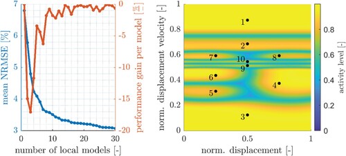Based on Figure 20 (left) the number of local models is set to $M=10$, which represents a trade-off between complexity and the performance improvement per additional local model. Figure 20 (right) exemplarily shows the final partitioning result of the normalised input space. It can be clearly derived, that both kinematic inputs are necessary to improve the model performance.

Figure 20. Influence of number of local models based on amplitude sweep and road a/b as training data (left), operating regions of local models based on amplitude sweep and road a/b as training data (right).

After identifying the coefficients of the Gaussians in Equation (18) by running the mentioned LoLiMoT algorithm with the system configuration defined above, the next step in the parameter identification process consists of the nonlinear constrained optimisation of each local linear model dynamics. For an efficient optimisation, it is crucial to determine a proper initial solution. Here, this is achieved by computing a Hammerstein model (i.e. $M=1$) based on a least square minimisation according to Ref. [32]. Furthermore, nonlinear constraints take numerical requirements into account, which are referring to enforce a stable system or a solver-specific stable integration as well as a solver-specific accuracy threshold. A hybrid use of optimisation methods is applied. At first, a global optimisation is performed by using the NOMAD algorithm [33] to further improve the initial solution based on one local linear model. Secondly, the coefficient set of this intermediate step is then used to run a local derivative-based sequential quadratic programming algorithm [34]. The resulting eigenvalues of the first-order local models including direct feedthrough of the system inputs are within the range of [−70; −40] $\text{rad/s}$.

Table 4 gives an overview of the model performance according to the objective value defined above. Several combinations of individual excitations were used to build a specific training dataset. Each of the resulting models was then tested with a particular excitation. At the bottom of the table, the mean values of different test combinations are stated. Overall, the use of sinusoidal amplitude sweep along with the real road excitation profiles are resulting in the lowest mean error and can be selected as dataset to sufficiently identify the system dynamics in ride comfort-related field of application. As it can be seen, the static and dynamic ramps show the highest deviation when not being part of the training dataset. Nevertheless, this behaviour can only be slightly improved when adding this information to the parameter identification procedure. It can be observed that the main difference occurs here in the course after the displacement peak. The force peak itself is accurately matching (low to medium displacement velocity) or is approx. 9% higher (high displacement velocity).

Table 4. Grey box model performance (NRMSE) based on different training and test data sets for M = 10 local linear models.

		Trained on
		Ampl. sweep	Ampl. sweep Road a/b	Ampl. sweep Dyn. ramps Road a/b	Ampl. sweep Dyn. ramps Road a/b Static ramps
Tested on	Static ramps	26.57%	19.47%	20.87%	16.54%
	Dynamic ramps	14.38%	9.17%	9.79%	9.08%
	Amplitude sweep	1.24%	2.10%	4.03%	5.02%
	Road a	10.37%	4.59%	4.82%	4.93%
	Road b	7.56%	3.84%	3.78%	4.90%
	Training data	1.24%	3.51%	5.61%	8.09%
	Combined w/o static ramps	8.39%	4.93%	5.61%	5.98%
	Combined	12.02%	7.83%	8.66%	8.09%

Discussion of the proposed model approaches

In this section, the presented model approaches are compared. The white box model is derived based on measurement data while the described pre-identification algorithm ensures a robust parameterisation process. It shows good results for the overall optimisation goal (NRMSE: 3.86%), consisting of the mean NRMSE of five excitation profiles. Especially synthetic stimulation profiles can be represented accurately. The generic grey box approach showed less accuracy for the combined training data (NRMSE: 8.09%) but can be optimised for harmonic and the real road excitations. Especially the static ramps can hardly be represented by the grey box approach. Here, the hysteresis of the compression and rebound stages cannot be sufficiently covered by the partitioning algorithm because of the low excitation velocities. It is assumed that the performance of the grey box model approach could be significantly improved by adding the proposed modified Dahl model of the white box approach to accurately match the static ramps. For the dynamic approaches, the grey box model interprets this as a dynamic hysteresis and can therefore represent those excitations with a scalable number of states. Furthermore, the valid and tested operating area is generally limited to the measurement data the grey box model is trained on (see Figure 8). An extrapolation of the activation functions in Figure 20 is carried out by clipping the normalised input space variables to the interval [0, 1]. The use of linear dynamic models allows an interpretation of potential responses at higher excitation frequencies and thus can be designed to match plausible physical behaviour accordingly.

Conclusion

In this contribution, we deal with modelling the jounce bumper of a passenger car in the context of road-induced ride comfort. First, we conducted full vehicle measurements to quantify the operating ranges of the jounce and created a generic measurement procedure. After presenting the measurement results, we showed two modelling approaches. The white box approach shows good modelling results for various types of excitations, whereby road-induced manoeuvres are captured with an accuracy (NRMSE) of 5.9% and 4.9%, respectively. In comparison, the generic grey box approach can be optimised to cover realistic dynamic excitations more precisely (4.8% and 3.8%) but shows less accuracy for the entire set of excitation profiles (on average 8.1%). Nevertheless, the approach is scalable in terms of computational effort and accuracy. In a simulation environment consisting of an accurate full-vehicle model, the presented models can be used for a virtual ride comfort assessment. This supports the reduction of hardware for the tuning of a vehicle’s driving behaviour.

Disclosure statement

No potential conflict of interest was reported by the author(s).

Notes

1 Because of that, optimizing the stiffnesses and the cut-off frequencies is preferable to optimizing the stiffnesses and the damping coefficients of the Maxwell elements. The first mentioned method leads to a linear optimization constraint, while the second mentioned approach causes a nonlinear constraint.

References

- Huber W. Industrie 4.0 in der Automobilproduktion. Wiesbaden: Springer Vieweg; 2016. doi:10.1007/978-3-658-12732-9.
- Wolf-Monheim F. CAE-based driving comfort optimization for passenger cars. In: Pfeffer PE, editor. 5th international Munich chassis symposium. Wiesbaden: Springer Vieweg; 2014. p. 133–149. doi:10.1007/978-3-658-05978-1_11.
- Badiru I, Cwycyshyn WB. Customer focus in ride development. SAE technical paper series. Proceedings; 2013.
- Wang Y, Ma Z, Wang L. A finite element stratification method for a polyurethane jounce bumper. Proc Inst Mech Eng D J Automob Eng. 2016;230:983–992.
- Röski K. Eine Methode zur simulationsbasierten Grundauslegung von PKW-Fahrwerken mit Vertiefung der Betrachtungen zum Fahrkomfort. München: Technische Universität München; 2012.
- Reimpell J, Betzler JW. Fahrwerktechnik: Grundlagen. 5th ed. Würzburg: Vogel; 2005.
- Kortüm W, Lugner P. Systemdynamik und Regelung von Fahrzeugen: Einführung und Beispiele. Springer eBook Collection Computer Science and Engineering. Berlin: Springer; 1994.
- Heissing B, Brandl HJ. Subjektive Beurteilung des Fahrverhaltens. Würzburg: Vogel fachbuch; 2002.
- Heißing B, Ersoy M, Gies S. Fahrwerkhandbuch: Grundlagen, Fahrdynamik, Komponenten, Systeme, Mechatronik, Perspektiven. 4th ed. Wiesbaden: Springer Vieweg; 2013.
- Wong JY. Theory of ground vehicles. 3rd ed. New York: John Wiley; 2001.
- Haigermoser A, Luber B, Rauh J, et al. Road and track irregularities: measurement, assessment and simulation. Veh Syst Dyn. 2015;53:878–957.
- ISO. Mechanical vibration – road surface profiles – reporting of measured data. Berlin: Beuth Verlag; 1995.
- Braun H. Messergebnisse von Straßenunebenheiten. VDI-Berichte Nr. 877. 1991:47–80.
- Karamihas S, Sayers M. The little book of profiling. Michigan: University of Michigan, Ann Arbor, Transportation Research Institute, Engineering Research Division; 1998.
- Agostinacchio M, Ciampa D, Olita S. The vibrations induced by surface irregularities in road pavements – a Matlab® approach. Eur Transp Res Rev. 2014;6:267–275.
- Rabiner LR, Schafer RW. Digital processing of speech signals. Prentice-Hall Signal Processing Series. Englewood Cliffs (NJ): Prentice-Hall; 1978.
- Brandt A. Noise and vibration analysis. Chichester: Wiley; 2011.
- Gillespie TD. Fundamentals of vehicle dynamics. 4th ed. Warrendale (PA): Society of Automotive Engineers; 1992.
- Eze MC, Eze VHU, Chidume C, et al. Review of the effects of standard deviation on time and frequency response of Gaussian filter. International Journal of Scientific & Engineering Research. 2016;7(9):749.
- Fornberg B. Generation of finite difference formulas on arbitrarily spaced grids. Math Comput. 1988: 699–706.
- Dahl PR. A solid frition model. El Segundo (CA): Aerospace Corp; 1968.
- Franklin GF, Powell JD. Digital control of dynamic systems. Reading (MA): Addison-Wesley; 1980.
- Butcher JC. Numerical methods for ordinary differential equations. Chichester: Wiley Blackwell; 2016.
- Dessort R, Meissner M, Kolmeder S, et al. Experimental nonlinear system identification of a shock absorber focusing on secondary ride comfort. In: Pfeffer P, editor. 12th international Munich chassis symposium 2021. Proceedings. Berlin: Springer Vieweg. doi:10.1007/978-3-662-64550-5_13
- Nelles O. Nonlinear system identification. Berlin: Springer; 2001.
- Nelles O. Nonlinear system identification with local linear neuro-fuzzy models. Aachen: Automatisierungstechnik, Shaker; 1999.
- Halfmann O, Nelles O, Holzmann H. Semi-physical modeling of the vertical vehicle dynamics. Proceedings of the American Control Conference; 1999.
- Rehrl J, Schwingshackl D, Horn M. A modeling approach for HVAC systems based on the LoLiMoT algorithm. IFAC Proc Vol. 2014;47(3):10862–10868.
- Nelles O, Fink A, Isermann R. Local linear model trees (LOLIMOT) toolbox for nonlinear system identification. IFAC Proc Vol. 2000;33(15):845–850.
- Lunze J. Regelungstechnik 1: Systemtheoretische Grundlagen, Analyse und Entwurf einschleifiger Regelungen. Berlin: Springer Vieweg; 2020. doi:10.1007/978-3-662-60746-6.
- Penrose R. A generalized inverse for matrices. Math Proc Cambridge Philos Soc. 1955;51(3):406–413.
- Brunton SL, Proctor JL, Kutz NJ. Discovering governing equations from data by sparse identification of nonlinear dynamical systems. Proc Natl Acad Sci USA; 113(15):3932–3937.
- Audet C, Dennis JE. Mesh adaptive direct search algorithms for constrained optimization. SIAM J Optim. 2006;17(1):188–217.
- Nocedal J, Wright SJ. Numerical optimization. Springer Series in Operations Research and Financial Engineering. New York: Springer; 2006. doi:10.1007/978-0-387-40065-5.