Asymmetric vehicle performance assessment using GG diagrams

Abstract

In closed-circuit racing such as NASCAR, vehicles often travel on highly-banked oval tracks that are dominated by left-hand corners. The aim of this paper is to study the generation and interpretation of the associated asymmetric GG diagrams and performance metrics. These include GG diagrams on inclined and/or cambered planar road surfaces, and GG diagrams on curved surfaces such as the interior face of an inverted cone. It is shown that a general fixed point on a traditional GG diagram is associated with acceleration or braking along a logarithmic spiral. Under pure acceleration and braking this spiral becomes a straight line, while under constant-speed cornering it becomes a circle. Some of these ideas are developed using a single-track car model. The paper then addresses the calculation and interpretation of GG-diagrams and performance metrics for a Generation 7 (Gen-7) NASCAR on curved road surfaces. The car's stability and performance limits under extreme lateral acceleration conditions are of particular interest. The main results come from a high-fidelity vehicle model and a representative set of parameters.

Keywords:

• GG diagrams
• optimal control
• road vehicle dynamics
• performance envelope
• NASCAR
• asymmetric vehicle performance

1. Introduction

The GG diagram is a standard tool that is used to determine the performance limit of road vehicles [1–3]. These diagrams establish the maximum steady-state longitudinal and lateral acceleration capabilities of the vehicle (car or motorcycle) at fixed speed, with the boundary representing the vehicle's physical limits. Families of GG diagrams, indexed by speed, are called GGV diagrams. These diagrams aim to predict the uncontrolled limits of the vehicle but do not address directly the driver's ability to control or drive it. Acceleration limits, especially in the longitudinal direction, are strongly dependent on speed. The physical inputs utilised by drivers are reported in Ref. [4], where so-called ‘willingness limits’ are presented using GG diagrams. These diagrams have also been used to assess the extent to which drivers utilise the full capabilities of the vehicle being driven [5].

The engine power and aerodynamic drag are the primary influence on the positive longitudinal acceleration limit, while the tyre grip and aerodynamic performance are the key factors determining the cornering and braking limits. In their traditional form, these diagrams relate to symmetric cars operating on horizontal planar road surfaces. Increases in the enclosed area of the GG envelope indicates a potential for enhanced performance. Such an area increase might be facilitated by a raft of parameter changes including the engine power, the suspension setup, tyre selections, changes to the car's aerodynamic characteristics, or the choice of differential configuration [6,7]. The regions where an area increase would be most beneficial are dependent on the track layout.

Early versions of the minimum-lap-time optimal control problem were solved using GG diagrams [8]. In Ref. [9], the vehicle is treated as a point mass, with prescribed acceleration limits, that is driven along an empirically determined ‘racing groove’. This is an example of a quasi-steady-state approach to minimum-lap-time control. The minimum transit time for a predefined trajectory is considered in Ref. [10] using a dynamic planar car model that includes longitudinal, lateral and yaw degrees-of-freedom. Once the track has been divided into sections using a series of curves, so-called critical points can be identified with their associated critical speeds .¹ To find the velocity profile, the equations of motion are integrated assuming maximum acceleration after each critical point and maximum deceleration before the following one. The resulting GG diagrams were compared with the performance measured for a Formula One car driven by professional racing drivers. More recently GG diagrams have found utility in solving the free-trajectory minimum-lap-time problem for both cars and motorcycles [11,12]. The overarching idea is to encapsulate the vehicle's capabilities in a GG diagram that summarises its performance envelope. These diagrams can be determined from either computer models, experiments or a combination of both.

The vehicle's handling and stability characteristics impact the driver's ability to operate the vehicle on its limits of performance. An unstable vehicle may undermine driver confidence, or in extreme cases, make it undriveable. In general terms, cars tend to become open-loop unstable and more difficult to control at high speed and/or under simultaneous braking and cornering. If it were possible, it would be most useful to be able to characterise the vehicle's stability characteristics across the entire GG diagram, as this would help predict the extent to which the driver is able to fully exploit the vehicle's performance. The treatment of stability over the full extent of the vehicle's performance envelope has produced several analysis techniques [1]. In other studies metrics are have been ‘borrowed’ from the aerospace industry –[13] investigates the use of stability derivatives, while the study [14] makes use of ‘jerk responses’ using differential geometric ideas. Nonlinear methods based on regions of attraction in the phase plane can be found in Ref. [15].

Straight running at constant speed, and constant-speed cornering are inherently equilibrium states that can be easily analysed using an eigenvalue analysis with linearised models [3,16]. When the vehicle operates under non-equilibrium conditions, the stability analysis becomes more nuanced, because the relationships between eigenvalues and stability is less clear. Indeed, control-theoretic notions such as ‘modes’, ‘resonant frequencies’ and ‘transfer functions’ lose their meaning.

To determine the vehicle stability over the interior of the operating regime it is necessary to develop methods of examining acceleration and braking under cornering – in these scenarios, the vehicle is no longer in equilibrium. To conduct this type of analysis the vehicle states along a prescribed trajectory are required. In simple straight-running cases one may find closed-form solutions to the vehicle's dynamic equations in terms of Bessel functions and the equations of motion need not be solved numerically [3,17]. One could also simulate the manoeuvre using a nonlinear vehicle model under feedback control in order to generate the desired motion [18].

An alternative approach is to determine the frozen-time vehicle state using a d'Alembert force system that acts as a surrogate for the forces of inertia experienced by the vehicle under acceleration or braking. In this approach, an accelerating or braking vehicle is approximated by one travelling at a constant speed but subjected to forces that capture the inertial effects of accelerating and braking; accelerating and braking can be ‘mimicked’ by travelling at constant speed up or down an incline. The frozen-time eigenvalues are then computed point-wise along a trajectory. This is the approach taken in the case of motorcycles in Ref. [18], with the domain of applicability of eigenvalue analysis discussed in Ref. [17]. In a more general scenario, one could consider a vehicle travelling on an incline that is also laterally cambered. In each of these scenarios, the vehicle remains in equilibrium and the vehicle states are deduced from algebraic equations of motion that contain additional terms representing the apparent forces.

The authors are of the opinion that the current literature relating to GG diagrams has three shortcomings that we aim to address:

• The vertical axis of the GG diagram is well understood to represent straight-line acceleration and braking, while the horizontal axis represents constant-speed cornering. The current interpretation of general interior points is that they represent some combination of the two, but the associated trajectory does not appear to be covered in the current literature. We show that general interior points correspond to trajectories on logarithmic spirals and illustrate how this information might be used to develop new performance metrics. One example is to adapt the ‘doghouse’ metric [19] from aerospace applications to road vehicles. We present a metric that is based on a prescribed manoeuvre describable by a small number of points within GG diagrams. This material is presented in Section 2.

• Almost all of the current literature is restricted to horizontal planar road surfaces, with [12] an exception. Motivated by applications in closed-circuit racing, we generalise these conventional ideas to include inclined and curved road surfaces such as the interior of a cone. In Section 3, we provide a summary of an optimal control approach to the computation of GG diagrams in Ref. [20], and analyse the computation of GG diagrams for single-track vehicle models on cambered planar road surfaces. A stability analysis of the vehicle at its limits of performance (on the periphery of the GG diagram) is presented that is based on an eigenvalue analysis. The section concludes with a performance metric that makes use of the transfer between the steering angle and the yaw-rate – the transfer function is evaluated on the perimeter of the GG diagram.

• The analysis techniques presented in Section 3 are extended to a high-fidelity model of a Gen-7 NASCAR specification vehicle in Section 4. Importantly, the vehicle studied here is asymmetric since the left- and right-hand sides of the car have different suspension stiffnesses and different tyres. This will lead to asymmetric GG diagrams even on planar-level road surfaces. A small-perturbation linear model for this vehicle is presented, with a conical road surfaces is included. We also show how the car's stability and steering response vary around the periphery of the GG diagram, and how vehicle set-up changes influence both stability and performance limits of the car.

The paper is concluded in Section 5.

2. Arbitrary points on the GG diagram

It is well understood that straight-line accelerating and braking, and steady-state cornering, are represented by the axes of the GG diagram. To access a general interior point on the GG diagram, it is necessary to accelerate/brake the vehicle under cornering. The purpose of this section is to discover the nature of the trajectories associated with arbitrary points on the GG diagram. A starting point for answering this question can be found in Chapter VI of Ref. [21] that deals with orbital problems containing central forces. These ideas were developed further in the context of a bicycle [22,23]. Suppose we wish a vehicle to follow a trajectory of fixed longitudinal acceleration $a_x$ and fixed lateral acceleration $a_y$. Setting the speed to $V=a_{x}t+V_0$ fixes $a_x$. For a given $a_y$, the car's instantaneous radius of curvature is (1) $\mathcal{R}=\frac{V^2}{a_y}$(1) with angular velocity (2) $\omega =\frac{a_y}{V}.$(2) Integrating (2(2) $\omega =\frac{a_y}{V}.$(2) ) with respect to time gives the yaw angle (3) $\alpha ={\int }_{V_0}^V\frac{a_y}{V}\frac{\mathrm{d}t}{\mathrm{d}V}\mathrm{d}V=\left(\frac{a_y}{a_x}\right)\ln \left(\frac{V}{V_0}\right).$(3) Solving (3(3) $\alpha ={\int }_{V_0}^V\frac{a_y}{V}\frac{\mathrm{d}t}{\mathrm{d}V}\mathrm{d}V=\left(\frac{a_y}{a_x}\right)\ln \left(\frac{V}{V_0}\right).$(3) ) for V and substituting into (1(1) $\mathcal{R}=\frac{V^2}{a_y}$(1) ) gives (4) $\mathcal{R}=\frac{V_0^2}{a_y}\exp \left(\frac{2a_x\alpha }{a_y}\right),$(4) which is the equation of a logarithmic spiral (in intrinsic coordinates).

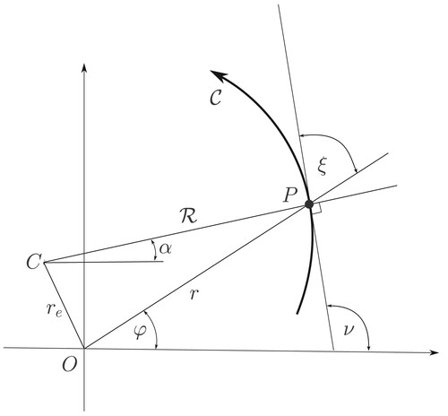
To express (4(4) $\mathcal{R}=\frac{V_0^2}{a_y}\exp \left(\frac{2a_x\alpha }{a_y}\right),$(4) ) in polar coordinates, a number of known properties of logarithmic spirals must be exploited. In the case of polar coordinate descriptions, logarithmic spirals are described by Ref. [24]: (5) $r(t)=\mathrm{Aexp}(\mathrm{B\phi }(t)),$(5) in which A and B are constants; see Figure 1. We will now link (4(4) $\mathcal{R}=\frac{V_0^2}{a_y}\exp \left(\frac{2a_x\alpha }{a_y}\right),$(4) ) and (5(5) $r(t)=\mathrm{Aexp}(\mathrm{B\phi }(t)),$(5) ) using the following known properties of logarithmic spirals. Referring to Figure 1:

1. The angle between the tangent to the spiral at an arbitrary point P, and the polar radius OP is given by (6) $\xi =\arctan \left(\frac{1}{B}\right).$(6)

2. It follows by simple geometry that φ and α differ by a fixed offset angle given by (7) $\alpha -\phi =\xi -\frac{\pi }{2}.$(7)

3. The centre of curvature is also a logarithmic spiral – described by (8) $r_e=\mathrm{ABexp}\left(B(\phi +\frac{\pi }{2})\right)$(8) with its centre located at C.

4. The spiral's radius of curvature $\mathcal{R}$ is given by: (9) $r=\mathcal{R}/\sqrt{1+B^2}.$(9)

Substituting (4(4) $\mathcal{R}=\frac{V_0^2}{a_y}\exp \left(\frac{2a_x\alpha }{a_y}\right),$(4) ) and (5(5) $r(t)=\mathrm{Aexp}(\mathrm{B\phi }(t)),$(5) ) into (9(9) $r=\mathcal{R}/\sqrt{1+B^2}.$(9) ) using (7(7) $\alpha -\phi =\xi -\frac{\pi }{2}.$(7) ) gives (10) $\begin{array}{rl}A& =\frac{V_0^2\exp \left(B(\xi -\frac{\pi }{2})\right)}{a_y\sqrt{1+B^2}}\end{array}$(10) (11) $\begin{array}{rl}B& =\frac{2a_x}{a_y}.\end{array}$(11) The distance travelled between the initial and final speeds can be found by integrating $\mathrm{ds}=\sqrt{r^2+{\left(\frac{\mathrm{d}r}{\mathrm{d}\phi }\right)}^2}\mathrm{d\phi },$which gives (12) $s=A\frac{\sqrt{1+B^2}}{B}{e}^{B(\frac{\pi }{2}-\xi )}({\left(\frac{V_f}{V_0}\right)}^2-1).$(12) Substituting for A and B gives the simple formula (13) $s=\frac{V_f^2-V_0^2}{2a_x},$(13) which is usually associated with rectilinear motion.

Figure 1. Relationship between intrinsic and polar co-ordinate descriptions of a logarithmic spiral. A generic vehicle path is given by $\mathcal{C}$ with a generic point P on it. The origin of the polar coordinate system is O, with r and φ the polar co-ordinates of P. The instantaneous centre of rotation of $\mathcal{C}$ at P is C. The instantaneous radius of curvature is $\mathcal{C}$, with α the angle between $\mathcal{C}$ and the horizontal x-axis. The angles ξ and ν define the orientation of a tangent to $\mathcal{C}$ at P with respect to r and the x-axis respectively.

In the case that $a_x>0$ and $a_y>0$ the spiral will diverge and rotate clockwise. If $a_x>0$ and $a_y<0$ the spiral will diverge and rotate anticlockwise. If $a_x<0$ and $a_y>0$ the spiral will converge and rotate clockwise. If $a_x<0$ and $a_y<0$ the spiral will converge and rotate anticlockwise. In the limit as $a_y\to 0$ the logarithmic spiral becomes a straight line, and in the limit $a_x\to 0$ the logarithmic spiral becomes a circle with the sense of rotation governed by the sign of $a_y$. A car's racing line can thus be approximated by ‘stitching together’ a sequence of circles, straight lines and converging/diverging logarithmic spirals.

Following the study [19], a performance metric could be based on the time taken to execute a specific set of manoeuvres, which are easily evaluated using GGV diagrams. Figure 2 illustrates an exemplar drivability metric (the total elapsed time) determined by only four points on a GG diagram. The characteristics of each section are given in Table 1.

Figure 2. An exemplar test course comprising a constant radius of turn at fixed speed section OA; an accelerating straight section AB; a section BC that describes braking into a tightening turn, and a section CD requiring acceleration out of a turn that ‘opens up’.

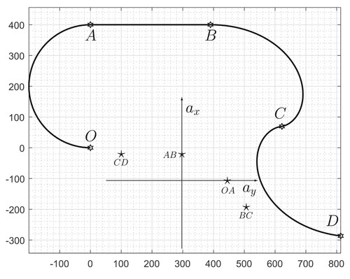
Table 1. Drivability metric.

Section	Speed range	$a_x$	$a_y$	Time	Distance
OA	50 m/s	0 m/s${}^2$	12.5 m/s${}^2$	$4\pi$ s	200 π m
AB	50 to 80 m/s	5 m/s${}^2$	0 m/s${}^2$	6 s	390 m
BC	80 to 30 m/s	$-5$ m/s${}^2$	15 m/s${}^2$	10 s	550 m
CD	30 to 80 m/s	5 m/s${}^2$	$-15$ m/s${}^2$	10 s	550 m

Note: The total elapsed time 38.5664 s.

3. An optimal control approach to computing a GG diagram

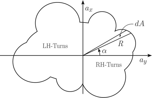
Traditional methods of computing GG diagrams rely on a sequence of discrete-point optimisation calculations that range over the extent of the GG diagram. This approach is tedious in terms of implementation and has been found vulnerable to jump discontinuities between sequential (local) minima. These problems were addressed in Ref. [20], where the GG diagram evaluation was recast as a single optimal control problem. As is standard, any errant behaviour in the optimal control calculation can be addressed using small regularisation terms in the performance index [3]. A slightly modified version of these ideas will be used here, which is then illustrated with a simple easy-to-follow single-track vehicle example. The performance criterion is motivated by the idea that the elemental area $\mathrm{dA}=\frac{1}{2}{R}^2(\alpha )\mathrm{d\alpha }$ (see Figure 3), can be integrated to find the total area enclosed by the GG diagram (14) $J=\frac{1}{2}{\int }_0^{2\pi }{R}^2(\alpha )\mathrm{d}\alpha .$(14) The optimal control problem is to maximise this area. It is clear that maximising the enclosed area is the same as minimising (15) $J=\frac{1}{2}{\int }_0^{2\pi }{R}^{-2}(\alpha )\mathrm{d}\alpha .$(15) In problems of this sort one must impose the state cyclicity constraint $x(0)=x(2\pi )$ on the problem states.

Figure 3. Abstract GG diagram with its periphery described in terms of polar coordinates.

The idea is to minimise J in (15(15) $J=\frac{1}{2}{\int }_0^{2\pi }{R}^{-2}(\alpha )\mathrm{d}\alpha .$(15) ), while satisfying the vehicle's steady-state equations of motion, constraints that keep the car on the road, tyre constraints, the assigned brake balance, the differential viscosity, and the car's aerodynamic performance which is linked to the vehicle's suspension's characteristics.

3.1. Single-track car model

For pedagogical purposes, we will begin by describing the car using a simple single-track car model. Models of this type have their genesis in Ref. [16], and are also analysed in some detail in Ref. [3]. The vehicle is assumed to be both-wheel driven. The body-fixed vehicle velocity components are given by (16) $\begin{array}{rl}u& =\mathrm{Vcos}\beta \end{array}$(16) (17) $\begin{array}{rl}v& =\mathrm{Vsin}\beta ,\end{array}$(17) where V is the vehicle speed and β its side-slip angle. The vehicle's steady-state yaw angular velocity is given in terms of its lateral acceleration $a_y=\mathrm{Rcos}\alpha$ by (18) ${\omega }_z=\mathrm{Rcos}\alpha /V,$(18) where R and α are given in polar coordinates (Figure 3). The front and rear side-slip angles are given by (19) $\begin{array}{rl}{\alpha }_r& =\mathrm{atan}2(v-{\omega }_{z}b,u)\end{array}$(19) (20) $\begin{array}{rl}{\alpha }_f& =\mathrm{atan}2(v+{\omega }_{z}a,u)-\delta ;\end{array}$(20) the car's geometric quantities are shown in Figure 4. The following equations describe the longitudinal and lateral equilibrium force balances (21) $\begin{array}{rl}0& =R(\sin \mathrm{\alpha cos}\beta -\cos \mathrm{\alpha sin}\beta )-F^x/M\end{array}$(21) (22) $\begin{array}{rl}0& =R(\cos \mathrm{\alpha cos}\beta +\sin \mathrm{\alpha sin}\beta )-F^y/M.\end{array}$(22) The longitudinal and lateral forces are given by (23) $\begin{array}{rl}{F}^x& =\cos \delta F_f^x-\sin \delta F_f^y+F_r^x+G_x-F_a^x\end{array}$(23) (24) $\begin{array}{rl}{F}^y& =\cos \delta F_f^y+\sin \delta F_f^x+F_r^y+G_y+F_a^y,\end{array}$(24) where the aerodynamic forces are given by (25) $\begin{array}{rl}& F_a^x=0.5\rho A_f{C}_D{u}^2\end{array}$(25) (26) $\begin{array}{rl}& F_a^y=0.5\rho A_f{C}_S{u}^2\end{array}$(26) (27) $\begin{array}{rl}& F_a^z=0.5\rho A_f{C}_L{u}^2,\end{array}$(27) in which the aerodynamic coefficients are initially taken as constant. The three components of gravity are given by (28) $\begin{array}{rl}{G}^x& =-\mathrm{gsin}\mu \end{array}$(28) (29) $\begin{array}{rl}{G}^y& =\mathrm{gsin}\mathrm{\varphi cos}\mu \end{array}$(29) (30) $\begin{array}{rl}{G}^z& =\mathrm{gcos}\mathrm{\varphi cos}\mu \end{array}$(30) where μ and ϕ are the roads inclination and camber angles respectively. The vertical force², and pitching and yaw moments must be constrained by (31) $\begin{array}{rl}0& =F_r^z+F_f^z+M{G}^z+F_a^z\end{array}$(31) (32) $\begin{array}{rl}0& =a{F}_f^z-b{F}_r^z-h{F}^x\end{array}$(32) (33) $\begin{array}{rl}0& =a(F_f^y\cos \delta +F_f^x\sin \delta )-b{F}_r^y.\end{array}$(33) The front ($F_f^x,F_f^y$) and rear ($F_r^x,F_r^y$) tyre forces are computed using nonlinear empirical formulas that are functions of the normal loads $F_f^z$ and $F_r^z$, the side-slip angles (19(19) $\begin{array}{rl}{\alpha }_r& =\mathrm{atan}2(v-{\omega }_{z}b,u)\end{array}$(19) ) and (20(20) $\begin{array}{rl}{\alpha }_f& =\mathrm{atan}2(v+{\omega }_{z}a,u)-\delta ;\end{array}$(20) ) and the longitudinal slips; see Ref. [25] and Appendix 1. The vehicle power is constrained by (34) $V(max(F_r^x,0)+max(F_f^x,0))/P_{max}\le 1.$(34) The GG diagram optimal control problem states are given by (35) $\mathit{x}=[R\beta \delta k_f{k}_r{]}^T,$(35) where $k_f$ and $k_r$ are the tyre longitudinal slips. The optimal controls are (36) $\mathit{u}=[R^{\prime }{\beta }^{\prime }{\delta }^{\prime }{k}_f^{\prime }{k}_r^{\prime }(F_f^z{)}^{\prime }(F_r^z{)}^{\prime }{]}^T,$(36) where the primes denote derivatives with respect to α (rather than time or elapsed distance).

Figure 4. Kinematics of a single-track car model showing its basic geometric parameters [3].

An optimal control code designed to maximise the area enclosed by the GG diagram was executed at variable vehicle speed, and on planar road surfaces of variable inclination and camber, with the results shown in Figure 5. The car and tyre parameters are given in Appendix 1.

Figure 5. Single-track car model operating at different speeds on inclined planar road surfaces. The left-hand figure shows the vehicle GGV diagram on a horizontal road surface at 70 m/s (red), 50 m/s (black) and 30 m/s (blue). The central figure shows the vehicle operating at 50 m/s on an inclined road surface with a ${25}^{\circ }$ inclination angle (red), a level road surface (black), and a ${25}^{\circ }$ declination angle (blue). The right-hand figure shows that vehicle operating at 50 m/s on a cambered road surface with a $-{25}^{\circ }$ camber angle (blue), a level road surface (black), and a ${25}^{\circ }$ camber angle (red).

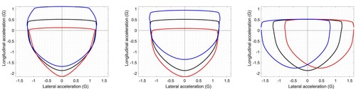
The left-hand figure shows that as the vehicle speed increases, the car's acceleration capability decreases, while its braking capacity is enhanced – both are due primarily to aerodynamic drag. On horizontal road surfaces the vehicle speed has little influence on its lateral acceleration capability. The centre figures show that travelling up an incline produces similar trends in the GG diagram boundaries. Again, an inclined road surface has little impact on the car's lateral acceleration capacity. The right-hand figure shows that road camber variations have the effect of translating the GG diagram sideways with little impact on the car's acceleration or braking performance.

3.2. Stability at the limit of performance

We conclude our brief analysis of the single-track car with a linear stability analysis at the vehicle's limit of performance. The equations of motion are linearised around an equilibrium operating condition described by $u_0$, $v_0$, ${\omega }_0$, ${\delta }_0$. This equilibrium point must be a point where the equations of motion are differentiable. When acceleration or braking is included, d'Alembert forces that act as surrogates for the real forces of inertia experienced under acceleration and braking must be recognised when determining the equilibrium state. The d'Alembert forces do not, however, appear in the linear equations of motion. The linear small-perturbation model used for the stability analysis here is (37) $A=\left[\begin{array}{ccc}{\displaystyle \frac{-C_f{\delta }_0(v_0+a{\omega }_0)}{m{u}_0^2}}& \frac{C_f{\delta }_0}{m{u}_0}+{\omega }_0& \frac{C_{f}a{\delta }_0}{m{u}_0}+v_0\\ {\displaystyle \frac{C{v}_0+\mathrm{Cs}{\omega }_0}{m{u}_0^2}-{\omega }_0}& -\frac{C}{m{u}_0}& \frac{-\mathrm{Cs}}{m{u}_0}-u_0\\ {\displaystyle \frac{\mathrm{Cs}{v}_0+C{q}^2{\omega }_0}{J{u}_0^2}}& \frac{-\mathrm{Cs}}{J{u}_0}& -\frac{C{q}^2}{J{u}_0}\end{array}\right]$(37) which is taken from Equation (4.53) in Ref. [3]. As a result of its small influence, we have thus neglected small variations in the vehicle's longitudinal speed, because these variations make no significant difference to the conclusions drawn in terms of stability or the vehicle's dynamic performance. Neglecting the longitudinal speed is tantamount to ignoring the first row and column of (37(37) $A=\left[\begin{array}{ccc}{\displaystyle \frac{-C_f{\delta }_0(v_0+a{\omega }_0)}{m{u}_0^2}}& \frac{C_f{\delta }_0}{m{u}_0}+{\omega }_0& \frac{C_{f}a{\delta }_0}{m{u}_0}+v_0\\ {\displaystyle \frac{C{v}_0+\mathrm{Cs}{\omega }_0}{m{u}_0^2}-{\omega }_0}& -\frac{C}{m{u}_0}& \frac{-\mathrm{Cs}}{m{u}_0}-u_0\\ {\displaystyle \frac{\mathrm{Cs}{v}_0+C{q}^2{\omega }_0}{J{u}_0^2}}& \frac{-\mathrm{Cs}}{J{u}_0}& -\frac{C{q}^2}{J{u}_0}\end{array}\right]$(37) ). When variations in the longitudinal speed are included, additional aerodynamics-related terms that come from (25(25) $\begin{array}{rl}& F_a^x=0.5\rho A_f{C}_D{u}^2\end{array}$(25) )–(27(27) $\begin{array}{rl}& F_a^z=0.5\rho A_f{C}_L{u}^2,\end{array}$(27) ) will appear in the first column. Terms of this type can be seen in the linearised model for the full car in Appendix 2.

The real and imaginary parts of the eigenvalues of linearised model evaluated around the periphery of the GG diagram are shown in Figure 6 .³ The left-hand part of Figure 6 shows the cornering stiffnesses for the linearised tyre model and the associated understeer coefficient. As is well known, the car is stable when the understeer coefficient (Equation (4.30) in Ref. [3]) is positive, and unstable above the vehicle's critical speed (Equation (4.33) in Ref. [3]) when the understeer coefficient is negative. On a level road surface, the tyres used in this study render the vehicle stable around the periphery of the GG diagram.

Figure 6. Single-track car model operating at 50 m/s on a horizontal road surface. The left-figure shows the front (red) and rear (blue) tyre cornering stiffnesses and the vehicle understeer coefficient (black). The right-hand figure shows the two-state linear model eigenvalues evaluated on the periphery of the GG diagram; the real parts are shown red and the imaginary parts blue.

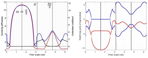
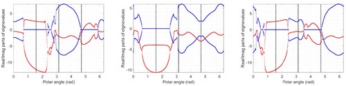
Figure 7 shows the destabilising influence of road camber. This loss of stability on cambered roads is due to changes in the tyre cornering stiffnesses brought about by lateral tyre-loading changes. In this case, stability is lost in the first and second quadrants of the GG diagram (i.e. under acceleration in straight running, and in right- and left-hand corners).

Figure 7. Stability eigenvalues on the periphery of the GG diagram at 50 m/s on a planar road surface. The real parts of the linearised model eigenvalues are shown in red, while the imaginary parts are illustrated in blue. The left-hand diagram corresponds to a road cambered at $-{25}^{\circ }$, the central plot is for a level road surface, while the right-hand diagram is for a road cambered at ${25}^{\circ }$.

3.3. A handling metric

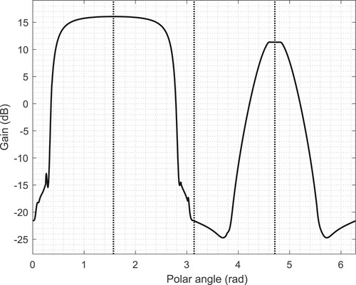
Figure 8 shows the steady-state gain of the transfer function mapping the steering angle to the yaw rate. It follows from the linear model that this steady-state transfer function is of the form $g(0)=\underset{s\to 0}{lim}C(\mathrm{sI}-A{)}^{-1}B=C{A}^{-1}B$ provided $g(s)$ is stable (the final-value theorem). Peaks are expected when A has eigenvalues near the origin. Clearly $g(0)$ has no meaning in the case that $g(s)$ is unstable because an arbitrarily small input will result in an unbounded response. That said, the real parts of the unstable eigenvalues speak to the extent to which these instabilities are controllable by the driver who acts as a low-bandwidth stabilising feedback controller. In this case, the steady-state yaw-rate response is maximum in straight-line braking and acceleration, while being de-emphasised under cornering.

Figure 8. Steady-state gain of the transfer function from the steering angle to the yaw rate for the vehicle operating at 50 m/s on a horizontal road surface.

4. Analysis of a Gen-7 NASCAR

We will now explore similar ideas in the context of a high-fidelity Gen-7 NASCAR model. The interested reader will find models of this type detailed in Ref. [26,27], where both the car and road surface models are described.

In connection with these models, several points are worth noting :

1. The car model includes a nonlinear suspension system that includes tyre squash. These details are required in order to compute the aerodynamic force and moment coefficients, which are responsive to the vehicle's orientation relative to both the air stream and road surface. The vehicle's distance from the road is also important;

2. The car is rear-wheel driven;

3. The car model has a limited-slip differential with an adjustable viscosity;

4. The car model has an adjustable brake balance ratio;

5. The braking torques on each axle are equal;

6. The tyres are described by empirical formulae of the type discussed in Ref. [25].

7. linearised car and tyre models were used in the stability analyses. These linear models were determined symbolically;

8. The slip and side-slip angle of each tyre are constrained within the tyre's practical operating range;

9. The steady-state model used in the optimal-control-based GG diagram calculations has states $\mathit{x}=[R\beta \delta k_{\mathrm{fr}}{k}_{\mathrm{fl}}{k}_{\mathrm{rr}}{k}_{\mathrm{rl}}{]}^T$and inputs $\mathit{u}=[R^{\prime }{\beta }^{\prime }{\delta }^{\prime }{k}_{\mathrm{fr}}^{\prime }{k}_{\mathrm{fl}}^{\prime }{k}_{\mathrm{rr}}^{\prime }{k}_{\mathrm{rl}}^{\prime }(F_{\mathrm{fr}}^z{)}^{\prime }(F_{\mathrm{fl}}^z{)}^{\prime }(F_{\mathrm{rr}}^z{)}^{\prime }(F_{\mathrm{rl}}^z{)}^{\prime }{]}^T.$

Again, the primes denote derivatives with respect to the GG diagram rotation angle α. In comparison with the states (35(35) $\mathit{x}=[R\beta \delta k_f{k}_r{]}^T,$(35) ) and inputs (36(36) $\mathit{u}=[R^{\prime }{\beta }^{\prime }{\delta }^{\prime }{k}_f^{\prime }{k}_r^{\prime }(F_f^z{)}^{\prime }(F_r^z{)}^{\prime }{]}^T,$(36) ) of the single-track car model, the number of slips and normal loads has doubled. 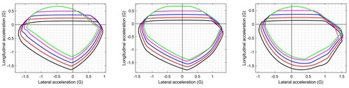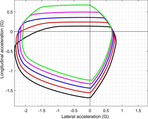The car's yaw velocity is again given by (38) ${\omega }_z=\mathrm{Rcos}\alpha /V.$(38) Figure 9 shows GGV diagrams of a Gen-7 NASCAR on planar road surfaces at different values of lateral road camber. Asymmetries in the suspension and tyre characteristics induce asymmetries in the GGV diagrams on both level and laterally cambered road surfaces. As the road surface camber varies from $-{25}^{\circ }$ towards ${25}^{\circ }$ the GGV diagrams move towards the right as expected. It is also evident from the level-road case that the car has been set up to favour negative lateral acceleration (for a negatively cambered oval track such as the Darlington speedway that is dominated by left-hand corners). Road cambering makes little difference to the car's straight-line acceleration capacity, which is determined primarily by the aerodynamic drag and the engine power. As the vehicle speed increases, the car's straight-line acceleration capability reduces, while its braking capacity is enhanced; both influences are due primarily to the car's aerodynamic performance. The car's lateral acceleration capability degrades at lower speeds – this is also predominantly an aerodynamic effect.

Figure 9. GGV diagrams for a Gen-7 NASCAR operating on planar road surfaces of variable lateral road camber; the left-hand figure is for $-{25}^{\circ }$ of camber, the centre figure is for a horizontal road surface and the right-hand figure is for ${25}^{\circ }$ of lateral road camber. The black plots correspond to the car travelling at 80 m/s; the red curves correspond to 70 m/s; the blue curves correspond to 60 m/s; the magenta curves are for 50 m/s and the green curves are for 40 m/s.

4.1. GG diagrams on a curved road surface

Our aim here is to obtain a broad overview of how road cambering on curved road surface can be expected to influence the GG diagram. Example 6.1 in Ref. [27] studies the curvature properties of a toroidal road surface and provides an example of a road surface that has curvature in both the y- and z-directions. The y-axis curvature generates centripetal force in the z-axis direction.

We now refer to the single-axle model illustrated in Figure 10. In this analysis, the vehicle is assumed to be travelling on the interior surface of a cone – the road is therefore assumed to have a curvature that gives rise to an angular velocity component in the vehicle's y-direction. This, in turn, produces an additional normal load on the tyres. The vehicle is also subject to gravitational and lateral accelerations. From this figure, we see that (39) $F^y=F_r^y+F_l^y=\mathrm{Rcos}\alpha -\sin \varphi ,$(39) where R and α have their usual meaning ($\mathrm{Rcos}\alpha$ is the lateral acceleration); ϕ is the road camber angle – M and G have been normalised. The total vertical tyre load is given by (40) $F^z=F_r^z+F_l^z=\mathrm{Rcos}\mathrm{\alpha tan}\varphi +\cos \varphi ,$(40) which shows that for a predominantly left-turning track ($\frac{\pi }{2}\le \alpha \le \frac{3\pi }{2}$) the road camber should be negative for maximum normal tyre loading. Taking moments around the left-hand wheel ground contact point gives (41) $F_r^z=\frac{1}{2}{F}^z-\frac{h}{w}{F}^y,$(41) which combined with (40(40) $F^z=F_r^z+F_l^z=\mathrm{Rcos}\mathrm{\alpha tan}\varphi +\cos \varphi ,$(40) ) gives (42) $F_l^z=\frac{1}{2}{F}^z+\frac{h}{w}{F}^y.$(42) For illustrative purposes, we suppose that the single-axle model has the normalised parameters given in Table 2.

Figure 10. Normal and lateral tyre loads as a function of the GG diagram sweep angle $0\le \alpha \le 2\pi$. The lateral acceleration is $\mathrm{Rcos}\alpha$ and the camber angle ϕ. All the car parameters are assumed normalised so that g = 1, M = 1, and R is in G's. All lengths are given as fractions of the vehicle length.

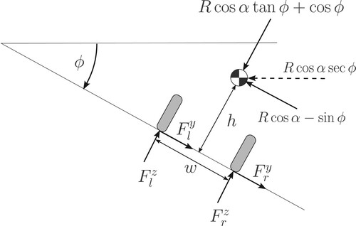
Table 2. Idealised and normalised tyre loading parameters.

R = 1.0

h = 0.15

w = 0.5

$\varphi =0^{\circ },\pm {20}^{\circ }$

For the parameters in Table 2, Figure 11 shows how the total lateral tyre force varies as a function of α. It is immediately evident that negative road camber has the effect of reducing the lateral tyre force requirement in left-hand corners (as compared to the $\varphi =0^{\circ }$ and $\varphi ={20}^{\circ }$ cases). For that reason, cars that are required to operate on predominantly left-turning tracks will have extended lateral acceleration capabilities if the track is negatively cambered. Put another way, ‘better vehicle performance can be expected when driving on the interior surface of a downward pointing cone as compared with driving on the exterior surface of the same cone when inverted.’

Figure 11. Total lateral tyre loads as a function of the sweep and camber angles, respectively α and ϕ. All the car parameters are assumed normalised so that g = 1, M = 1, and R is in G's. The black curve corresponds to $\varphi =0^{\circ }$. The red curve is for $\varphi ={20}^{\circ }$, while the blue curve represents the $\varphi =-{20}^{\circ }$ case.

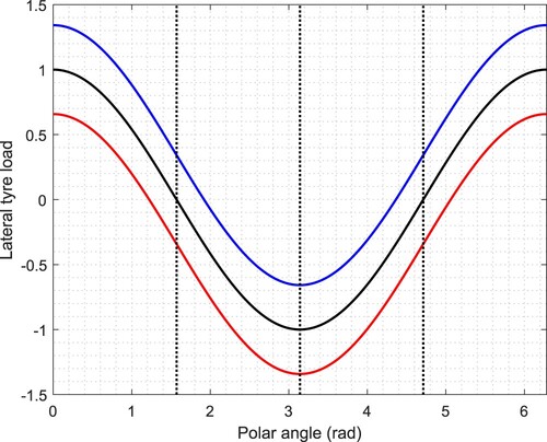
Figure 12 shows how the right- and left-hand tyre loads vary with lateral acceleration. Under high lateral acceleration, the right-hand tyre is most heavily loaded when the car is turning left on a negatively cambered road. This increased normal loading tends to increase the right-hand tyre's lateral force-generating capability. Under positive road camber conditions, the left-hand tyre would tend to lift from the road.

Figure 12. Idealised left- and right-hand tyre normal loads for varying road camber; the left-hand plot is for the left-hand tyre. The black curves are for a level road. The red curve represents a road camber of ${15}^{\circ }$, while the blue curve is for a road camber of $-{15}^{\circ }$.

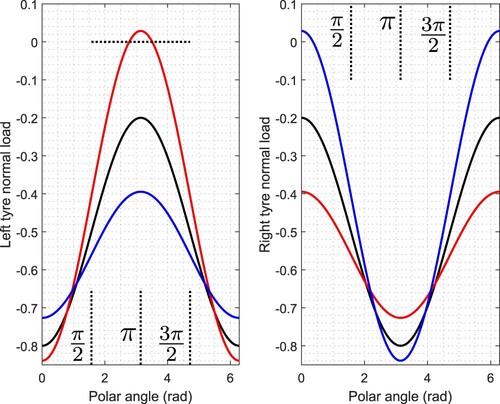
Figure 13 shows the normal load behaviour of the NASCAR model at 50 m/s as one moves around the perimeter of the GG diagram for three different road inclination angles. For the purpose of these calculations, the road surface is assumed to be conical (and is thus ‘curved’). These diagrams show that the right- and left-hand tyre loads are in broad conformity with Figure 12. As with Figure 12, the right-hand tyres show increased normal loads for negative camber angles. The left-hand tyre loading is reduced in left-hand corners, but the trends in the tyre loads with road camber are not reproduced as in Figure 12. This may be caused by various influences including aerodynamic loading, brake saturation, the influence of the differential and so on. Also, the full model is for a two-axle vehicle rather than a single-axle approximation and $R(\alpha )\ne R$ as in Figure 12. Both analyses are predicting a left-hand tyre to ‘go light’ under high lateral accelerations in left-hand corners.

Figure 13. Tyre normal loads for a Gen-7 NASCAR travelling at 50 m/s. The black plot corresponds to the car operating on a horizontal road surface. The red plot corresponds to the car operating on a road surface with ${20}^{\circ }$ of camber. The blue plot corresponds to the car operating on a road surface with $-{20}^{\circ }$ of camber.

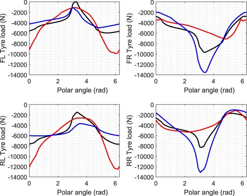
Figure 14 shows a GGV diagram for a Gen-7 NASCAR operating at variable speed on a conical road surface with a camber angle of $-{20}^{\circ }$. When comparing these plots with those in the left-hand part of Figure 9, the influence of road curvature is evident producing a significantly higher lateral acceleration capacity in left-hand corners. Road curvature has left the vehicle's longitudinal and lateral acceleration capability in right-hand turns relatively unaffected.

Figure 14. GGV diagrams for a Gen-7 NASCAR operating on a conical road surface with a camber angle of $-{20}^{\circ }$. The black plots corresponds to the car travelling at 80 m/s; the red curves corresponds to 70 m/s; the blue curves corresponds to 60 m/s; the magenta curves are for 50 m/s and the green curves are for 40 m/s.

We conclude this section by validating, qualitatively, the results given above using measured data obtained from a Gen-6 NASCAR [26]. Before doing that, we will describe briefly the relevant differences between Gen-6 and Gen-7 cars. Gen-6 cars were optimised to race on left-turning, highly-banked ovals. As a result, these cars are ‘stretched’ at the rear to have asymmetric body shapes [28]. Gen-7 vehicles, on the other hand, moved towards a more symmetric body shape. This was motivated in part by the introduction of more road courses into the racing calendar that reduced the need for a car design that focussed exclusively on left-turning high-speed ovals. Aerodynamically speaking, one of the significant changes when moving to Gen-7 was the removal of side skirts which was a way of generating significant downforce by exploiting high-speed under-car air flows. Referring to Figure A3 in Ref. [26], we see that the downforce coefficient for a Gen-6 car operating on Darlington is $C_L\approx 1.2$, whereas the downforce coefficient for a Gen-7 car on the same oval is $C_L\approx 0.7$; this represents a 40% reduction. Figure 15 shows the measured normal tyre loads for a single lap of the Darlington Raceway for a Gen-6 car [26]. As the car enters left-hand corners, it experiences high lateral accelerations and rolls to the right producing a three-fold increase in the normal tyre loads on the right-hand tyres. These sections of high lateral acceleration correspond to a dense cluster of data points in the second quadrant of the GG diagram; see Figure 16.

Figure 15. Measured normal tyre loads captured on an instrumented Gen-6 NASCAR on the Darlington Raceway.

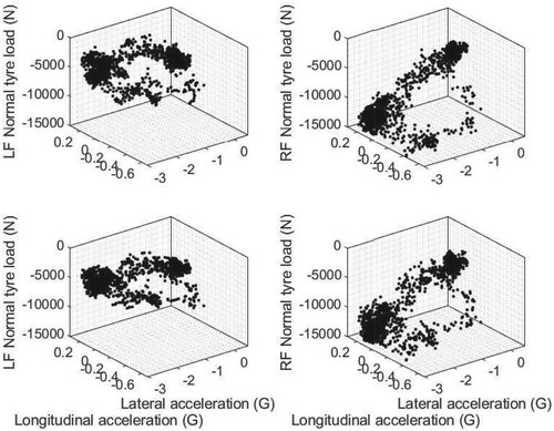
Figure 16. Measured lateral and longitudinal accelerations captured on an instrumented Gen-6 NASCAR on the Darlington Raceway.

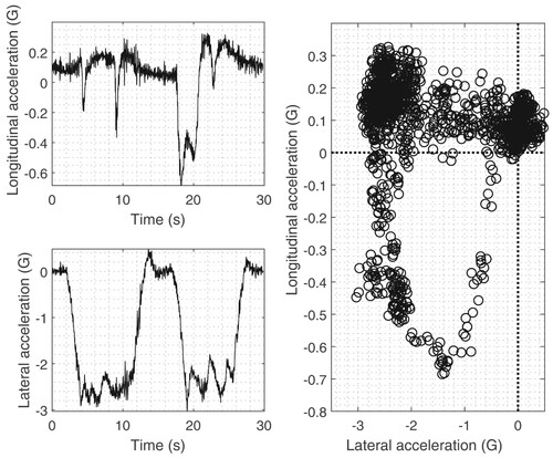
Figure 16 shows the measured lateral and longitudinal accelerations for a Gen-6 NASCAR measured on Darlington. Almost all of the cornering is left-handed with lateral accelerations reaching almost $-3G$; these high lateral accelerations are enabled by high downforces. The longitudinal accelerations are predominantly positive but reach $-0.6G$ under braking into Turn 3. The associated diagram is dominated by modest longitudinal acceleration combined with high lateral accelerations in left-hand corners.

4.2. Vehicle stability

The stability of the car was analysed using a linearised version of the high-fidelity car model that includes operating-point-dependent aerodynamic coefficients. Some of these details are provided in Appendix 2, with further information available in Refs [26,27]. The linearised model is again evaluated along the perimeter of the GG diagram. A linearised model description considers variations in the longitudinal speed, the lateral speed and the yaw velocity. The first column of the A-matrix corresponds to the longitudinal speed variations, while the second and third columns correspond to the lateral and yaw velocity variations respectively. Since the influence of longitudinal speed variations are ‘small’ (as with the single-track car model), the stability results presented here are based on the two-dimensional $(2,2)$ block of the A-matrix in Appendix 2. 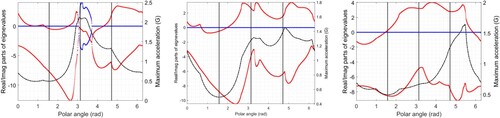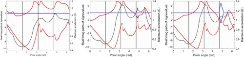The matrix entries are a function of $u_0$, $v_0$, ${\delta }_0$, ${\omega }_0$, the tyre normal loads and the corresponding tyre cornering stiffnesses. The tyre model is a combined-slip model with its cornering stiffnesses a function of the normal load, and the longitudinal and side-slip angles. The eigenvalues of the two-state linearised model evaluated around the periphery of the GG diagram are shown in Figure 17. In the case of a horizontal road surface (the central plot in Figure 17), the car is stable in the first quadrant of the GG diagram, as well as parts of the second and fourth quadrants. The stable region in the second quadrant is a set-up requirement for a car being driven on a predominantly left-turning track such as the Darlington oval. When the track is horizontal and planar, the vehicle is stable for $-{16}^{\circ }\le \alpha \le {132}^{\circ }$. In the case of an adversely cambered track (the right-hand plot of Figure 17), the stable range becomes $-{23}^{\circ }\le \alpha \le {83}^{\circ }$. The most significant reduction occurs in the second quadrant of the GG diagram. From the left-hand part of Figure 17 (negative camber) it is seen that the vehicle is stable for $-{30}^{\circ }\le \alpha \le {145}^{\circ }$. The region of apparent stability in the range ${137}^{\circ }\le \alpha \le {239}^{\circ }$ is illusory because in this interval the tyres are operating on their adhesion limit, are their associated linearised models cannot be relied on. This is evidenced by the fact that the car's lateral acceleration in left-hand corners is over 2 G (see Figure 14). The normal loads on the right-hand tyres are in excess of 12 kN, while the side forces on the right-hand tyres are in excess of 11 kN.

Figure 17. Eigenvalue plots for a Gen-7 NASCAR operating at 50 m/s on a conical road surface. The real parts of the linearised model eigenvalues are shown in red, while the imaginary parts are illustrated in blue. The black dot-dash curve is the maximum achievable acceleration as the GG diagram is traversed. The left-hand figure is for $-{20}^{\circ }$ of road camber, the central figure is for a horizontal road surface and the right-hand figure is for ${20}^{\circ }$ of camber.

4.3. Steady-state response curves

Other performance indicators that may find practical utility are the steady-state gains of frozen-time transfer functions. Frozen-time transfer functions must be computed and interpreted under the assumption that constant-speed models augmented with acceleration-related inertial forces adequately represent the real physics of the problem.

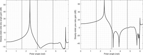
To find these transfer functions we need state-space B- and C-matrices for selected inputs and outputs. For example, we consider small steering angle perturbations as input, and the car's corresponding yaw velocity and side-slip angle responses as outputs. These matrices are computed by linearising the car's nonlinear equations of motion and are given in Appendix 2. The steady-state responses are given by $g(0)=C{A}^{-1}B$. Figure 18 shows strong responses under hard acceleration in left-hand corners, and modest braking in right-hand corners. Both peaks are due to near-zero eigenvalues of the A-matrix at these values of α. If the frozen-time model used here is a reasonable representation of the car's physical behaviour, these figures indicate the possibility of ‘twitchy’ handling behaviour when accelerating in left-hand corners and braking in right-hand ones. We remind the reader that this is an open-loop response prediction that may be controlled by the driver.

Figure 18. Steady-state steer angle gains for a Gen-7 NASCAR operating at 50 m/s on a horizontal planar road surface. The left-hand figure is the yaw-rate gain, while the right-hand figure is the side-slip angle gain.

4.4. Set-up changes

Our final results demonstrate the use of GG-diagram analysis in examining the effect of vehicle set-up changes. Figure 19 illustrates the effect of moving the brake balance towards the front axle. In the nominal set-up, 68% of the braking torque is applied to the front axle. It is evident that increasing the brake bias further towards the front axle is detrimental to the car's braking performance. Not unexpectedly, neither change influences the GG diagram in the first two quadrants. However, in the second and third quadrants, the car's braking capability is reduced by moving the brake bias towards the front axle. Not shown – when the braking torques is moved rearwards towards equal-axle braking, the car's braking performance is significantly degraded.

Figure 19. Brake balance for a Gen-7 NASCAR travelling at 50 m/s. The left-hand figure is for a level road surface. The right-hand figure is for a curved road surface with $-{20}^{\circ }$ of camber. The black plot corresponds to the car operating with 67% of the braking torque applied to the front axle. The red plot corresponds to the car operating with 80% of the braking torque applied to the front axle. The blue plot corresponds to the car operating with 90% of the braking torque applied to the front axle.

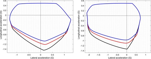
Figure 20. Stability due to variable brake balance for a Gen-7 NASCAR travelling at 50 m/s on a level road surface. The real parts of the linearised model eigenvalues are shown in red, while the imaginary parts are illustrated in blue. The black dot-dash curve is the maximum achievable acceleration as the GG diagram is traversed. The left-hand figure corresponds to a nominal brake balance of 67% on the front wheels. The central figure corresponds to a nominal brake balance of 80% on the front wheels. The right-hand figure corresponds to a nominal brake balance of 90% on the front wheels.

The influence of the brake balance adjustments on the stability of the car operating on a level surface is illustrated in Figure 20. It is important to note that these plots correspond to equilibrium points on the periphery of the GG diagram, where the front tyres are sometimes operating on the longitudinal slip limit. As a result, both the GG diagrams and their associated stability plots can be highly sensitive to the limits placed on the tyre slip and side-slip angles in the optimal control problem. A high degree of sensitivity was experienced in this case. The nominal case corresponds to 67% of the braking occurring on the front wheels (the left-hand part of the figure). In this case, the car is stable on the GG diagram periphery between 0.7 and 1.9 rad, with an acceleration capability of between 1.2 and 1.45 G in left-hand turns. This apparent lack of stability is for the uncontrolled car. If the instability growth rate is not too high, this instability may be, even subconsciously, controlled by the driver. When the brake balance is changed to 80% on the front axle, the car's stability improves marginally, but at the cost of a degraded braking performance in left-hand turns. When the brake balance is changed to 90% on the front brakes, there is little change in the stability of the car, but one observes a further degradation in the vehicle's braking performance in left-hand turns, where the capability is reduced to between 1.3 and 0.95 G.

The effect of other parameter changes such as differential viscosity and mass centre location can be studied in much the same way.

5. Conclusion

The GG diagram is routinely employed to assess the performance limits of road vehicles operating on planar level road surfaces. The focus of this work is to extend these ideas to racetracks with inclined, cambered or curved running surfaces. Inclination changes may involve ‘tilting’ the planar road surface, or they could involve the introduction of curved road surfaces – toroidal and conical surfaces are two obvious examples. If curved road surfaces are employed, the equations used to compute GG diagrams must recognise the additional steady-state centrifugal forces generated by road curvature.

When the road surface is level and planar, and the car has fixed longitudinal and lateral acceleration, we show that the car's trajectory approximates a logarithmic spiral. This insight can be used to develop track-specific performance metrics that are describable by a small number of points on the GG diagram. It is possible to use these metrics to identify critical parts on the GG map boundary where performance improvements might be of benefit.

We then use a single-track model to illustrate the influence of road inclination and camber on the performance limits of road vehicles. A linearised model is used to examine the car's stability properties around the periphery of the GG diagram. This study acts as a precursor to analysing the GG characteristics of a Gen-7 NASCAR on tilted and/or curved road surfaces.

A single-axle model is used to illustrate the influence of road curvature on the tyres' normal and lateral load distribution, and hence on the GG diagram. In the case of the car under investigation here, it is shown that for a road without curvature speed and inclination variations have little impact of the car's lateral acceleration capabilities, while lateral road camber variations have a significant impact on the lateral positioning of the GG diagram. Camber variations also influence the vehicle's stability properties along its performance-limit boundary. Asymmetries in the GGV diagrams are due to asymmetries in the suspension system and the tyres; in the case of NASCAR-specification vehicles – in this case, all four tyres are different. The impact of road curvature has a significant impact on the extent of the GGV diagrams. Strong contributors to these effects are a combination of tyre normal load transfers and the vehicle's aerodynamic characteristics.

Since the stability analysis given here is open-loop, the unstable car may still be controllable by a skilled driver. Steady-state transfer function analysis indicates that the NASCAR's handling may become ‘twitchy’ under left-hand cornering, with stabilising driver intervention required under heavy braking. The utility of the GG diagram is also demonstrated when assessing the impact of set-up changes on the vehicle's limit of performance. Brake balance changes were examined as examples.

Disclosure statement

No potential conflict of interest was reported by the author(s).

Notes

1 The terms critical speed and critical point are taken from Ref. [10]: ‘The critical point of a turn is the point that limits the maximum curve constant velocity (critical speed) in that curve.’

2 In the analysis given here, we assume that the car is travelling on a planar road surface that may be inclined and/or cambered. In some cases one may wish to analyse GG-type performance limits on curved surfaces – the interior surface of a cone for example, which would be appropriate for studies focussed on NASCAR ovals. Curved road surfaces introduce steady-state centripetal forces that must be accommodated in the performance analysis. More is said about this in Section 4.1

3 Referring to Figure 3, we associate the positive $a_y$-axis with $\alpha =0$, the positive $a_x$-axis with $\alpha =\frac{\pi }{2}$ and so on. These α-related angles have been marked explicitly on Figure 6 but will be replaced thereafter by three unmarked vertical lines corresponding to $\alpha =\frac{\pi }{2}$, $\alpha =\pi$ and $\alpha =\frac{3\pi }{2}$. This has been done to reduce diagrammatic clutter.

Appendices

Appendix 1.

Simple car and tyre model parameters

The parameters for the simple single-track model are given in Table A1. The non-linear tyre model used is described in detail in Ref. [25], and the parameters used in this model are given in Table A2.

Table B1. Single-track car model parameters.

Symbol	Description	Value
m	Vehicle mass	720 kg
J	Yaw moment of inertia	450 kg m${}^2$
w	Vehicle length	3.4 m
a	Distance from the mass centre to the front axle	1.6 m
b	Distance from the mass centre to the rear axle	1.8 m
h	Mass centre height	0.35 m
$C_D$	Drag coefficient	0.4
$C_S$	Side-force coefficient	0.0
$C_L$	Down-force coefficient	0.2
$P_{max}$	Maximum engine power	250 kW

Table B2. Single-track car model parameters.

Symbol	Description	Value
$F_{z1}$	Normal load reference 1	2 kN
$F_{z2}$	Normal load reference 2	6 kN
${\mu }_{x1}$	Peak longitudinal friction coefficient at load 1	1.75
${\mu }_{x2}$	Peak longitudinal friction coefficient at load 2	1.40
${\mu }_{y1}$	Peak lateral friction coefficient at load 1	1.80
${\mu }_{y2}$	Peak lateral friction coefficient at load 2	1.45
${\kappa }_1$	Slip coefficient at peak friction at load 1	0.11
${\kappa }_2$	Slip coefficient at peak friction at load 2	0.10
${\alpha }_1$	Slip angle at peak friction at load 1	$9^{\circ }$
${\alpha }_2$	Slip angle at peak friction at load 2	$8^{\circ }$
$Q_x$	Longitudinal shape factor	1.9
$Q_y$	Lateral shape factor	1.9

Appendix 2.

Linearised model

The purpose of this appendix is to provide a brief description of the high-fidelity model used to analyse the performance of a Gen-7 NASCAR. A dynamic model for a car travelling on a flat include road surface can be described in terms of three degrees of freedom – two translational and one rotational: (A1) $\begin{array}{rl}\dot{u}& =v{\omega }_z+\frac{F_x}{m}+G_x\end{array}$(A1) (A2) $\begin{array}{rl}\dot{v}& =-u{\omega }_z+\frac{F_y}{m}+G_y,\end{array}$(A2) where $G_x$ and $G_y$ are the longitudinal components of gravity expressed in body-fixed coordinates. The car's angular acceleration is described by (A3) ${\dot{\omega }}_z=\frac{M_z}{J_{\mathrm{zz}}}.$(A3) Under cornering and/or curved road surface conditions, the longitudinal and lateral dynamics given in (A1(A1) $\begin{array}{rl}\dot{u}& =v{\omega }_z+\frac{F_x}{m}+G_x\end{array}$(A1) ) and (A2(A2) $\begin{array}{rl}\dot{v}& =-u{\omega }_z+\frac{F_y}{m}+G_y,\end{array}$(A2) ) interact, and the tyre longitudinal slips and side-slip angles are no longer zero. Combined-slip empirical formulae are used to determine the magnitude of the lateral tyre forces as functions of the tyre side-slip angle, the longitudinal slip and normal load. That is: (A4) $F^y=f(\alpha ,\kappa ,F^z).$(A4) Linearising the lateral tyre forces gives the following cornering stiffness expressions (A5) $C_{\ast \ast }={\frac{\mathrm{\partial }{F}^y}{\mathrm{\partial }\alpha }|}_{{\alpha }_0,{\kappa }_0,F_0^z},$(A5) where the asterisks are used as reference labels for each of the four tyres. For small-angle variations, the tyre side-slip angles cornering are given by (A6) $\begin{array}{rl}{\alpha }_{\mathrm{fr}}& =\delta -(a{\omega }_z+v)/(u-{\omega }_z{w}_f);{\alpha }_{\mathrm{fl}}=\delta -(a{\omega }_z+v)/({\omega }_z{w}_f+u);\\ {\alpha }_{\mathrm{rr}}& =-(v-b{\omega }_z)/(u-{\omega }_z{w}_r);{\alpha }_{\mathrm{rl}}=-(v-b{\omega }_z)/(u+{\omega }_z{w}_r),\end{array}$(A6) while the tyre forces are given by (A7) $F_{\mathrm{fr}}^y=C_{\mathrm{fr}}{\alpha }_{\mathrm{fr}};F_{\mathrm{fl}}^y=C_{\mathrm{fl}}{\alpha }_{\mathrm{fl}};F_{\mathrm{rr}}^y=C_{\mathrm{rr}}{\alpha }_{\mathrm{rr}};F_{\mathrm{rl}}^y=C_{\mathrm{rl}}{\alpha }_{\mathrm{rl}};$(A7) the cornering stiffnesses are given by (A5(A5) $C_{\ast \ast }={\frac{\mathrm{\partial }{F}^y}{\mathrm{\partial }\alpha }|}_{{\alpha }_0,{\kappa }_0,F_0^z},$(A5) ).

For small steering angles, the longitudinal and lateral external forces and the external yaw moment are given by (A8) $\begin{array}{rl}{F}^x& =F_{\mathrm{fr}}^x+F_{\mathrm{fl}}^x+F_{\mathrm{rr}}^x+F_{\mathrm{rl}}^x-\delta (F_{\mathrm{fr}}^y+F_{\mathrm{fl}}^y)-\frac{1}{2}\rho A_f{C}_D{u}^2\\ F^y& =F_{\mathrm{fr}}^y+F_{\mathrm{fl}}^y+F_{\mathrm{rr}}^y+F_{\mathrm{rl}}^y+\delta (F_{\mathrm{fr}}^x+F_{\mathrm{fl}}^x)+\frac{1}{2}\rho A_f{C}_S{u}^2\\ M^z& =a(F_{\mathrm{fr}}^y+F_{\mathrm{fl}}^y+\delta (F_{\mathrm{fr}}^x+F_{\mathrm{fl}}^x))-b(F_{\mathrm{rr}}^y+F_{\mathrm{rl}}^y)\\ & +w_f(F_{\mathrm{fl}}^x-F_{\mathrm{fr}}^x+\delta (F_{\mathrm{fr}}^y-F_{\mathrm{fl}}^y))+w_r(F_{\mathrm{rl}}^x-F_{\mathrm{rr}}^x)+\frac{1}{2}\rho A_f{M}_A^z{u}^2.\end{array}$(A8) Equations (A1(A1) $\begin{array}{rl}\dot{u}& =v{\omega }_z+\frac{F_x}{m}+G_x\end{array}$(A1) ) to (A8(A8) $\begin{array}{rl}{F}^x& =F_{\mathrm{fr}}^x+F_{\mathrm{fl}}^x+F_{\mathrm{rr}}^x+F_{\mathrm{rl}}^x-\delta (F_{\mathrm{fr}}^y+F_{\mathrm{fl}}^y)-\frac{1}{2}\rho A_f{C}_D{u}^2\\ F^y& =F_{\mathrm{fr}}^y+F_{\mathrm{fl}}^y+F_{\mathrm{rr}}^y+F_{\mathrm{rl}}^y+\delta (F_{\mathrm{fr}}^x+F_{\mathrm{fl}}^x)+\frac{1}{2}\rho A_f{C}_S{u}^2\\ M^z& =a(F_{\mathrm{fr}}^y+F_{\mathrm{fl}}^y+\delta (F_{\mathrm{fr}}^x+F_{\mathrm{fl}}^x))-b(F_{\mathrm{rr}}^y+F_{\mathrm{rl}}^y)\\ & +w_f(F_{\mathrm{fl}}^x-F_{\mathrm{fr}}^x+\delta (F_{\mathrm{fr}}^y-F_{\mathrm{fl}}^y))+w_r(F_{\mathrm{rl}}^x-F_{\mathrm{rr}}^x)+\frac{1}{2}\rho A_f{M}_A^z{u}^2.\end{array}$(A8) ) were linearised (with Maple) to find the state-space matrices for a small-perturbation linear model: (A9) $\begin{array}{rl}{A}_{11}& =-{\delta }_0(\frac{C_{\mathit{fr}}(a{\omega }_0+v_0)}{m{(u_0-{\omega }_0{w}_f)}^2}+\frac{C_{\mathit{fl}}(a{\omega }_0+v_0)}{m(u_0+{\omega }_0{w}_f{)}^2})-\frac{\rho A_f{C}_D{u}_0}{m}\end{array}$(A9) (A10) $\begin{array}{rl}{A}_{12}& ={\omega }_0+{\delta }_0(\frac{C_{\mathit{fr}}}{m(u_0-{\omega }_0{w}_f)}+\frac{{\delta }_0{C}_{\mathit{fl}}}{m(u_0+{\omega }_0{w}_f)})\end{array}$(A10) (A11) $\begin{array}{rl}{A}_{13}& =v_0+{\delta }_0{w}_f(\frac{C_{\mathit{fr}}(a{\omega }_0+v_0)}{m{(u_0-{\omega }_0{w}_f)}^2}-\frac{C_{\mathit{fl}}(a{\omega }_0+v_0)}{m{(u_0+{\omega }_0{w}_f)}^2})\\ & +{\delta }_{0}a(\frac{C_{\mathit{fr}}}{m(u_0-{\omega }_0{w}_f)}+\frac{C_{\mathit{fl}}}{m(u_0+{\omega }_0{w}_f)})\end{array}$(A11) (A12) $\begin{array}{rl}{A}_{21}& =-{\omega }_0+(a{\omega }_0+v_0)(\frac{C_{\mathit{fr}}}{m{(u_0-{\omega }_0{w}_f)}^2}+\frac{C_{\mathit{fl}}}{m{(u_0+{\omega }_0{w}_f)}^2})\end{array}$(A12) (A13) $\begin{array}{rl}& -(b{\omega }_0-v_0)(\frac{C_{\mathit{rr}}}{m{(u_0-{\omega }_0{w}_r)}^2}+\frac{C_{\mathit{rl}}}{m{({\omega }_0{w}_r+u_0)}^2})+\frac{\rho A_f{C}_S{u}_0}{m}\end{array}$(A13) (A14) $\begin{array}{rl}{A}_{22}& =-\frac{C_{\mathit{fr}}}{m(u_0-{\omega }_0{w}_f)}-\frac{C_{\mathit{fl}}}{m(u_0+{\omega }_0{w}_f)}-\frac{C_{\mathit{rr}}}{m(u_0-{\omega }_0{w}_r)}-\frac{C_{\mathit{rl}}}{m(u_0+{\omega }_0{w}_r)}\end{array}$(A14) (A15) $\begin{array}{rl}{A}_{23}& =-u_0-w_f(\frac{C_{\mathit{fr}}(v_0+a{\omega }_0)}{m(u_0-{\omega }_0{w}_f{)}^2}-\frac{C_{\mathit{fl}}(v_0+a{\omega }_0)}{m(u_0+{\omega }_0{w}_f{)}^2})\\ & +w_r(\frac{C_{\mathit{rr}}(b{\omega }_0-v_0)}{m(u_0-{\omega }_0{w}_r{)}^2}+\frac{C_{\mathit{rl}}(v_0-b{\omega }_0)}{m(u_0+{\omega }_0{w}_r{)}^2})\\ & -a(\frac{C_{\mathit{fr}}}{m(u_0-{\omega }_0{w}_f)}+\frac{C_{\mathit{fl}}}{m(u_0+{\omega }_0{w}_f)})\\ & +b(\frac{C_{\mathit{rr}}}{m(u_0-{\omega }_0{w}_r)}+\frac{C_{\mathit{rl}}}{m(u_0+{\omega }_0{w}_r)})\\ A_{31}& =a(\frac{C_{\mathit{fr}}(v_0+a{\omega }_0)}{J_{\mathrm{zz}}(u_0-{\omega }_0{w}_f{)}^2}+\frac{C_{\mathit{fl}}(v_0+a{\omega }_0)}{J_{\mathrm{zz}}(u_0+{\omega }_0{w}_f{)}^2})\\ & -b(\frac{C_{\mathit{rr}}(v_0-b{\omega }_0)}{J_{\mathrm{zz}}(u_0-{\omega }_0{w}_r{)}^2}+\frac{C_{\mathit{rl}}(v_0-b{\omega }_0)}{J_{\mathrm{zz}}(u_0+{\omega }_0{w}_r{)}^2})\\ & +{\delta }_0{w}_f(\frac{C_{\mathit{fr}}(a{\omega }_0+v_0)}{J_{\mathrm{zz}}(u_0-{\omega }_0{w}_f{)}^2}-\frac{C_{\mathit{fl}}(a{\omega }_0+v_0)}{J_{\mathrm{zz}}(u_0+{\omega }_0{w}_f{)}^2})+\frac{\rho A_f{M}_A^x{u}_0}{J_{\mathrm{zz}}}\end{array}$(A15) (A16) $\begin{array}{rl}{A}_{32}& =-a(\frac{C_{\mathit{fr}}}{J_{\mathrm{zz}}(u_0-{\omega }_0{w}_f)}+\frac{C_{\mathit{fl}}}{J_{\mathrm{zz}}(u_0+{\omega }_0{w}_f)})\\ & +b(\frac{C_{\mathit{rr}}}{J_{\mathrm{zz}}(u_0-{\omega }_0{w}_r)}+\frac{C_{\mathit{rl}}}{J_{\mathrm{zz}}(u_0+{\omega }_0{w}_r)})\\ & -{\delta }_0{w}_f(\frac{C_{\mathit{fr}}}{J_{\mathrm{zz}}(u_0-{\omega }_0{w}_f)}-\frac{C_{\mathit{fl}}}{J_{\mathrm{zz}}(u_0+{\omega }_0{w}_f)})\end{array}$(A16) (A17) $\begin{array}{rl}{A}_{33}& =-a^2(\frac{C_{\mathit{fr}}}{J_{\mathrm{zz}}(u_0-{\omega }_0{w}_f)}+\frac{C_{\mathit{fl}}}{J_{\mathrm{zz}}(u_0+{\omega }_0{w}_f)})\\ & -b^2(\frac{C_{\mathit{rr}}}{J_{\mathrm{zz}}(u_0-{\omega }_0{w}_r)}+\frac{C_{\mathit{rl}}}{J_{\mathrm{zz}}(u_0+{\omega }_0{w}_r)})\\ & -{\delta }_{0}a{w}_f(\frac{C_{\mathit{fr}}}{J_{\mathrm{zz}}(u_0-{\omega }_0{w}_f)}-\frac{C_{\mathit{fl}}}{J_{\mathrm{zz}}(u_0+{\omega }_0{w}_f)})\\ & -a{w}_f(\frac{C_{\mathit{fr}}(v_0+a{\omega }_0)}{J_{\mathrm{zz}}(u_0-\omega w_f{)}^2}-\frac{C_{\mathit{fl}}(a{\omega }_0+v_0)}{J_{\mathrm{zz}}(u_0+\omega w_f{)}^2})\\ & +b{w}_r(\frac{C_{\mathit{rr}}(v_0-b{\omega }_0)}{J_{\mathrm{zz}}(u_0-{\omega }_0{w}_r{)}^2}-\frac{C_{\mathit{rl}}(v_0-b{\omega }_0)}{J_{\mathrm{zz}}(u_0+{\omega }_0{w}_r{)}^2})\\ & -{\delta }_0{w}_f^2(\frac{C_{\mathit{fr}}(v_0+a{\omega }_0)}{J_{\mathrm{zz}}(u_0-{\omega }_0{w}_f{)}^2}+\frac{C_{\mathit{fl}}(v_0+a{\omega }_0)}{J_{\mathrm{zz}}(u_0+{\omega }_0{w}_f{)}^2})\end{array}$(A17) The input matrix corresponding to the small steering angle perturbations $\mathrm{\Delta }\delta$ is given by (A18) $\begin{array}{rl}{B}_1& =\frac{-2{\delta }_0}{m}(C_{\mathit{fr}}+C_{\mathit{fl}})+\frac{C_{\mathit{fr}}(v_0+a{\omega }_0)}{m(u_0-{\omega }_0{w}_f)}+\frac{C_{\mathit{fl}}(v_0+a{\omega }_0)}{m(u_0+{\omega }_0{w}_f)}\end{array}$(A18) (A19) $\begin{array}{rl}{B}_2& =\frac{C_{\mathit{fr}}+C_{\mathit{fl}}+F_{\mathrm{fr}}^x+F_{\mathrm{fl}}^x}{m}\end{array}$(A19) (A20) $\begin{array}{rl}{B}_3& =\frac{a}{J_{\mathrm{zz}}}(C_{\mathit{fr}}+C_{\mathit{fl}}+F_{\mathrm{fr}}^x+F_{\mathrm{fl}}^x)+\frac{2w_f{\delta }_0}{J_{\mathrm{zz}}}(C_{\mathit{fr}}-C_{\mathit{fl}})\\ & +\frac{w_f{C}_{\mathit{fl}}}{J_{\mathrm{zz}}}\left(\frac{v_0+a{\omega }_0}{u_0+{\omega }_0{w}_f)}\right)-\frac{w_f{C}_{\mathit{fr}}}{J_{\mathrm{zz}}}\left(\frac{v_0+a{\omega }_0}{u_0-{\omega }_0{w}_f)}\right).\end{array}$(A20) The output matrices corresponding to small yaw-velocity perturbations $\mathrm{\Delta }{\omega }_z$ and small side-slip angle perturbations $\mathrm{\Delta }\beta$ are given by (A21) $C_1=\left[\begin{array}{ccc}0& 0& 1\end{array}\right]$(A21) and (A22) $C_2=\left[\begin{array}{ccc}{\displaystyle \frac{-v_0}{u_0^2}}& {\displaystyle \frac{1}{u_0}}& 0\end{array}\right]$(A22) respectively, since $\beta \approx \frac{v}{u}$.

Small perturbations in the longitudinal velocity introduce a third eigenvalue in the linearised vehicle models that is typically ‘small’. This third eigenvalue has only a minor influence on the conclusions drawn relating to vehicular stability. For that reason, for both the single- and double-track vehicles studied here, we have neglected the $\frac{\mathrm{\partial }\cdot }{\mathrm{\partial }u}$ terms in these models. These terms correspond to the first row and column of the $3\times 3$ A-matrices describing the linear vehicle dynamics. If desired, the full model can easily be employed.

References

- Milliken WF, Milliken DL. Race car vehicle dynamics. Warrendale (PA): SAE; 2005.
- Brayshaw D, Harrison M. A quasi steady state approach to race car lap simulation in order to understand the effects of racing line and centre of gravity location. Proc Inst Mech Eng D: J Automobile Eng. 2005;219(6):725–39. doi: 10.1243/095440705X11211
- Limebeer D, Massaro M. Dynamics and optimal control of road vehicles. Oxford: Oxford University Press; 2018.
- Bartlett W, Masory O. Driver abilities in closed course testing. J Passeng Cars: Mech Syst J. 2000;109(6):395–407.
- Rice R. Measuring car-driver interection with the g-g diagram. SAE Technical Paper 730018, 1973, doi: 10.4271/730018
- Tremlett A, Assadian F, Purdy D, et al. Quasi-steady-state linearisation of the racing vehicle acceleration envelope: a limited slip differential example. Veh Syst Dyn. 2014;52(11):1416–42. doi: 10.1080/00423114.2014.943927
- Tremlett A, Massaro M, Purdy D, et al. Optimal control of motorsport differentials. Veh Syst Dyn. 2015;53(12):1772–1794. doi: 10.1080/00423114.2015.1093150
- Massaro M, Limebeer DJN. Minimum-lap-time optimisation and simulation. Veh Syst Dyn. 2021;59(7):1069–1113. doi: 10.1080/00423114.2021.1910718
- Roland RD TC. Computer simulation of watkins glen grand prix circuit performance, Tech. Rep. ZL-5002-K-1, Cornell Aeronautical Laboratory. 1971.
- Metz D, Williams D. Near time-optimal control of racing vehicles. Automatica. 1989;25(6):841–57. doi: 10.1016/0005-1098(89)90052-6
- Veneri M, Massaro M. A free-trajectory quasi-steady-state optimal-control method for minimum lap-time of race vehicles. Veh Syst Dyn. 2020;58(6):933–954. doi: 10.1080/00423114.2019.1608364
- Lovato S, Massaro M. A three-dimensional free-trajectory quasi-steady-state optimal-control method for minimum-lap-time of race vehicles. Veh Syst Dyn. 2022;60(5):1512–1530. doi: 10.1080/00423114.2021.1878242
- Radt H, Dis DV. Vehicle handling responses using stability derivatives. SAE Technical Paper (960483). 1996.
- Yi J, Li J, Lu J, et al. On the stability and agility of aggressive vehicle maneuvers: a pendulum-turn maneuver example. IEEE Trans Control Syst Technol. 2012;20(3):663–676. doi: 10.1109/TCST.2011.2121908
- Masouleh MI, Limebeer DJN. Region of attraction analysis for nonlinear vehicle lateral dynamics using sum-of-squares programming. Veh Syst Dyn. 2017;56(7):1118–1138. doi: 10.1080/00423114.2017.1409429
- Pacejka HB. Tire and vehicle dynamics. 3rd ed. Oxford: Butterworth Heinemann; 2012.
- Salisbury IG, Limebeer DJN, Tremlett A, et al. The unification of acceleration envelope and driveability concepts. In: 24th International Symposium on Dynamics of Vehicles on Road and Tracks (IAVSD), Graz, Austria: International Association for Vehicle System Dynamics (IAVSD); 2015.
- Limebeer DJN, Sharp RS, Evangelou S. The stability of motorcycles under acceleration and braking. J Mech Eng Sci. 2001;215(9):1095–109. doi: 10.1177/095440620121500910
- III GR, Downing DR. Evaluation of several agility metrics for fighter aircraft using optimal trajectory analysis. J Aircr. 1995;32(4):732–738. doi: 10.2514/3.46784
- Massaro SLM, Veneri M. An optimal control approach to the computation of g-g diagrams. Veh Syst Dyn. 2024;62(2):448–462. doi: 10.1080/00423114.2023.2178467
- Routh EJ. A treatise on dynamics of a particle. Cambridge: Cambridge University Press; 1898.
- Routh GRR. The motion of a bicycle. Messenger Math. 1899;28:151–169.
- Limebeer DJN, Sharma A. Burst oscillations in the accelerating bicycle. J Appl Mech. 2010;77(6):061012. doi: 10.1115/1.4000909
- Lockwood EH. A book of curves. Cambridge: Cambridge University Press; 1961.
- Perantoni G, Limebeer DJN. Optimal control of a formula one car with variable parameters. Veh Syst Dyn. 2014;52(5):653–78. doi: 10.1080/00423114.2014.889315
- Limebeer DJN, Bastin M, Warren E, et al. Optimal control of a NASCAR specification race car. Veh Syst Dyn. 2023;61(5):1210–1235. doi: 10.1080/00423114.2022.2067573
- Limebeer DJN, Warren E. A review of road models for vehicular control. Veh Syst Dyn. 2023;61(6):1449–1475. doi: 10.1080/00423114.2022.2085582
- Jacuzzi E. Developing NASCAR's Gen-7 aerodynamics, Race Car Engineering. 2022.