Unproductive Activities and the Rate of Surplus Value at the Industry Level in Korea, 1995–2015

ABSTRACT

In order to explain how the Korean economy underwent structural change through the two crises of 1997– 1998 and 2008 within the context of globalisation, this article focuses on class analysis and inter-sectoral value transfer by estimating the sectoral rates of exploitation along with the sectoral monetary expressions of labour time. Our data indicate the possibility that the expansion of unproductive activities, accompanied by intensification of exploitation within the unproductive sectors, might not have overtaken capital accumulation in Korea during 1995–2015. It can also be concluded that the condition for manufacturing’s capital accumulation steadily improved since the 1997–1998 crisis but started to deteriorate after 2011. Our value-theoretic analysis provides a foundation for understanding the context of the regime change, which may plausibly characterise the Korean economy in the last couple of decades.

KEY WORDS:

• Sectoral rates of surplus value
• unproductive labour
• monetary expression of labour time
• Korean economy

The momentum of the neo-liberal structuration of the Korean economy critically accelerated as a result of the 1997–1998 financial crisis. The two decades since that crisis have seen an enormous increase in non-regular employment through the flexibilisation of the labour market, which deepens income inequality, and an ever-increasing importance of financial elements in everyday life as well as in capital accumulation. Suffice it to say that the 2008 global financial crisis gave further impetus to these tendencies.

With high exposure to globalisation, the internationalisation of productive capital such as foreign direct investment (FDI) and market opening came to be crucial explanatory factors for the change in the rate of profit (Hong 2013). At the same time, some favourable conditions were established for the conventional export-led growth strategy; export-biased productivity growth, suppression of wages and an undervalued exchange rate (Uni 2017).

In this setting, it is important to explain how the Korean economy underwent structural change through the two crises of 1997–1998 and 2008 within the context of economic globalisation. We approach this challenging task from a Marxian perspective focusing upon the distinction between productive and unproductive activities and the estimation of the rate of surplus value at the industry level. This article aims to provide a sketch of the structural change in the Korean economy during 1995–2015 by providing indicators based upon the Marxian labour theory of value.

The main contributions of this article are summarised in two points. First, we estimate Marxian ratios of the Korean economy both at the macro level and the sectoral level within the framework of the “New Interpretation” (NI) of Marxian value theory as presented in Duménil (1980) and Foley (1982). Based on the central thesis of the Marxian labour theory of value that money value added is the result of expenditure of living labour, the NI proposes to accept the equivalence between the two at the aggregate level as an axiom. The associated proportionality coefficient – called the monetary expression of labour time – can be used in converting between price categories and Marx’s labour value categories, thereby allowing one to recover the latter directly from the former. This has opened new areas of research in Marxian literature to empirically test Marx’s hypotheses and estimate Marxian ratios, using readily available real world data such as national income accounts, as in this article.¹

When applying the NI to the Korean data, we explicitly consider the distinction between productive and unproductive labours and the decomposition of the income of self-employed into capital income and labour income. The latter is crucial since the share of the self-employed sector in the Korean economy is significantly high at around 30% of the total working population during 1995-2015. In the literature of Marxian value theory, labour income of the self-employed is usually counted as a wage equivalent (Shaikh and Tonak 1994). Considering that most self-employed persons have scarce opportunity for average salaried jobs, however, this approach necessarily tends to underestimate the rate of surplus value. The per capita income of the self-employed started to fall short of the average income of wage workers around 1993 in Korea. Since then, the gap between the two has been widening continuously, except for the short period of the 1997–1998 crisis.

Second, based on confirmation, through panel unit root tests, that the hypothesis of equalisation of the sectoral rates of surplus value does not hold for the Korean economy during 1995–2015, we propose a novel approach to estimate the rate of surplus value at the industry level that relies on the method of the “inverse transformation” of price variables into value variables. More specifically, we initially estimate the labour share in income of each productive industry – which is a price variable – by using the approach suggested in Joo and Jeon (2014), and then use it to derive the sectoral rates of surplus value, which is a value variable.

As we incorporate the decomposition of income of the self-employed sector to the estimation of the sectoral rates of exploitation, there may be an objection that the self-employed do not produce surplus value as they are not “capitalistically employed.” However, it can be safely said that they are subsumed under the overarching nexus of the capital–labour relation. In particular, many of them are “economically dependent workers” in that their labour processes are controlled and supervised by capital, although their legal statuses are the “self-employed” (Oostveen et al. 2013).

The rest of the article is organised as follows. In the next section we first compute Piketty’s (2014) capital–income ratio for the Korean economy and provide an alternative reading based upon the capital–labour class analysis; for this, we conduct profit rate analysis for the entire economy and the manufacturing industry. In the following section, Marxian value ratios at the macro-economic level are measured. Marxian value ratios at the industry level are estimated in the subsequent section before we conclude the article.²

An Alternative Reading of Piketty

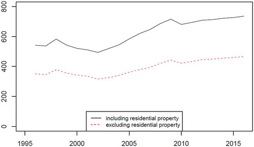
We begin by outlining how inequality in the Korean economy has developed through neo-liberal structuration. The global phenomena of the expansion of income and wealth inequality pointed out by Piketty (2014) has been markedly observed in Korea as well during 1995–2015. As shown in Figure 1, Piketty’s β (that is, capital–income ratio) declined in the aftermath of the 1997–1998 crisis and started to rise considerably in early 2000.³ It decreased somewhat right after the 2008 global crisis but has continued to exhibit an upward trend.

Figure 1. Piketty’s , 1995–2016

Note: We used private non-financial assets for capital and, for income, net national income.

Income distribution can be examined from a different perspective in relation to productivity and profitability of capital by relying on the following decomposition formula of the rate of profit:

(1)

where r, K, P, and Y, denote the rate of profit, capital stock, profits and output, respectively. The evolutions of r, , capital productivity, and , profit share, during the sample period are illustrated in Figure 2.⁴ Figure 2 confirms Rieu and Joo’s (2014) result on the profit rate dynamics of the Korean economy; that is, that a rise in profit share constantly offset a decline in capital productivity thereby preventing the falling tendency of the rate of profit from unfolding. In other words, the strengthening of capital’s class power played a vital role in avoiding the tendency of the profit rate to fall. This dynamic has changed since 2010 when capital productivity levelled off and both the rate of profit and the capital share in income started to decrease.

Figure 2. The rate of profit, capital productivity, and profit share: all industries, 1995–2016 (1995=1)

Note: Capital = structures + equipment. Capital can be measured differently; for instance, net financial assets can be added or residential property can be subtracted. No alternative combination made any significant difference to the trends.

In all, Figures 1 and 2 indicate that the capital–income ratio, the profit share and the rate of profit shared the similar secular trend during the whole sample period. This result partly corresponds to Piketty’s thesis on the co-movement of the wealth–income ratio and profit share. Piketty (2014, 220) suggests that the positive correlation between the two is due to an elasticity of substitution being greater than one. However, data collected in the literature contradict Piketty’s argument, making it empirically weak (see, for example, Semieniuk 2017). Rather, that the class struggle developed in favour of capital through neo-liberal structuration provides a better explanation at least for the Korean economy during this period.

As can be seen in Figure 3, manufacturing is still a dominant and growing industry in Korea. While the world and Korea’s major trading partners experienced a decline in the share of manufacturing in GDP during 1995–2015, it increased in Korea during the same period except for the period after 2011. By implication, understanding the performance of the manufacturing industry would provide an essential clue in explaining the structural change of the Korean economy which took place during 1995–2015.

Figure 3. Manufacturing’s value added as a percentage of GDP, South Korea and other major traders, 1995–2017

Source: World Bank data.

In this setting, the profit rate of manufacturing is analysed in the similar manner as above and the result is reported in Figure 4.⁵ There are a couple of interesting results to note in comparison to the case of the whole economy. First, manufacturing’s capital productivity stabilised after the 1997–1998 crisis, which contrasts to the significant downfall of capital productivity in the case of the whole economy. Second, the upward trend of the profit share of manufacturing is more pronounced than that of entire industries. As a consequence, manufacturing’s profitability has been stronger and less volatile than that of the whole economy. Over the entire sample period, it has witnessed an upward trend followed by stabilisation until 2011 when it started to fall; however, the decline was not as severe as that of the whole economy.

Figure 4. The rate of profit, capital productivity, and profit share: manufacturing, 1995–2016 (1995=1)

Note: Capital = structures + equipment + intellectual property products.

By inspecting the average annual rates of change of each variable, the entire sample period can be divided into two sub-periods, 1996–2010 and 2011–2015, while the first sub-period can be further divided into 1996–1998 and 1999–2010, as summarised in Table 1.

Table 1. The annual rates of change of the rate of profit, capital productivity and profit share, whole economy and manufacturing, 1996–2015 (%)

	Whole economy			Manufacturing
	Profit rate	Capital productivity	Profit share	Profit rate	Capital productivity	Profit share
1996–2010	-0.1	-2.42	2.12	3.2	-0.79	3.8
1996–1998	-13.11	-8.24	-5.3	-0.44	-8.46	8.55
1999–2010	3.15	-0.96	3.96	1.12	2.61	2.61
2011–2015	-2.42	-0.4	-2.02	-7.7	-2.01	-5.85

Source: See appendix.

In examining these periods, several points can be made. First, the impact of the 1997–1998 crisis on the profitability of manufacturing, reflected in the average annual rate of -0.44% during 1996–1998, was mild compared to -13.1% for the whole economy, whereas the consequence for capital productivity was fatal for both the whole economy and manufacturing, -8.24% and -8.46%, respectively. It was due to the considerably strong profit share, 8.55%, the manufacturing industry achieved during this crisis episode.

Second, the sub-period 1999–2010 was a long phase of recovering from, and reversing, the crisis effects on profitability and productivity of capital for both manufacturing and the economy; but this trend was more pronounced in the manufacturing sector. In either case, however, the recovery of the profit rate from the 1997–1998 crisis was possible mainly due to the profit share.

Third, the increase in the profitability of manufacturing at the average annual rate of 3.2% during 1996–2010 stands out in comparison to -0.10% for the whole economy. Note that this happened when the capital productivity not only of the whole economy but also of manufacturing recorded a negative average annual rate of change. Contrarily, the period 2011–2015 is marked by a rapid fall of manufacturing’s profitability at the pace of -7.7% amidst stagnant performance of both the profit rate and capital productivity across industries. This can be explained by the fact that manufacturing witnessed a solid profit share, 3.8% during 1996–2010, whereas it recorded the worst number for its profit share, -5.85%, during 2011–2015.

The empirical observations thus far point to the importance of the dynamics of class conflict reflected in the profit share. In particular, several differences documented above between manufacturing and entire industries will provide crucial insights in understanding structural change in the Korean economy.

Marxian Value Analysis: Macro–Level

To further pursue our discussion from the previous section on the effect of class conflict on the distribution of national income, we study historical developments of Marxian ratios in the Korean economy, such as the value of labour power and the rate of exploitation at the macro–level from the perspective of the NI of Marxian value theory. In comparison to our discussion in the previous section, we add two extensions. First, the distinction between productive and unproductive labours is explicitly incorporated into the analysis.⁶ This distinction is specific to the Classical and Marxian theories of value. Even in the literature on Marxian value theory, some are sceptical about the logical consistency and the analytical usefulness of the distinction (see, for example, Laibman 1999). However, as shown later, some characteristic patterns of the capital accumulation in Korea can be captured using this distinction. We adopt the conventional definition of productive labour as “wage labour that exchanges against capital and is employed in the productive phase of the circuit of capital rather than in the realisation or financial phases” (Foley 2013, 261).

Second, considering the fact that the share of the self-employed, unincorporated sector is large in the Korean economy and that the social and economic conditions of the self-employed are quite weak, we decompose the income of this sector – which is officially categorised as profit – into capital income and labour income when measuring the income distribution. In doing this, we follow Joo and Jeon (2014) and decompose mixed income, which is another name for the income of the self-employed sector, according to the ratio between capital income and labour income in the incorporated sector.⁷

To begin with, according to the NI, the value of labour power (VLP) and the rate of exploitation, denoted by e, are defined as follows⁸:

(2)

(3)

where w denotes a wage rate and m the monetary expression of labour time (MELT). When computing the exploitation rate and the value of labour power according to equations (2) and (3), we measure the two key parameters, w and m, by explicitly considering the productive–unproductive labour distinction along with the decomposition of the mixed income. In the case of w, on the one hand, it is not the total wage of the whole economy that is counted but only of the productive sectors plus the labour share of the mixed income. Let us denote the latter by , which then should replace w in equations (2) and (3).

On the other hand, with the definition of the MELT being the ratio between aggregate value added and total labour time, there are two issues that can be considered related to the denominator of the MELT. First, one can count ① only productive labours as in Mohun (2006) and Cogliano (2017) or ② the entire labours, productive or unproductive. ① is a more standard approach in Marxian literature and it is consistent with Foley (1986). Second, one can Ⓐ take the productive–unproductive labour distinction as equivalent to the productive–unproductive industry distinction as in Cogliano (2017) or Ⓑ apply the class concept to the productive–unproductive labour distinction thereby categorising supervisory labour as unproductive as in Mohun (2006). In this article, we adopt the ①-Ⓐ combination.⁹ In addition, we take the labour of the self-employed as productive. In all, denoting the aggregate monetary value added by MVA and total labour time of the whole productive sectors and those of the whole unproductive sectors, respectively, by L_P and L_U, the MELT can be expressed as where .

In order to visualise the consequence of counting the labour of the self-employed in the denominator of the MELT as productive, we illustrate in Figure 5 two different versions of the MELT, one that counts the labour of the self-employed as productive and the other that does not. In either case, the MELT constantly rises until 2011 after which it slows down and stagnates. Yet the gap between the two measures of the MELT tends to widen after the 1997–1998 crisis. This result partly reflects that the productivity of the self-employed sector has been sluggish.

Figure 5. The monetary expression of labour time, 1995–2015

Note: We used net national income for the aggregate money value added in the numerator of the MELT and the total labour time of the productive industries is computed by “the annual number of employed and self-employed x monthly average of working time x 12” for the productive industries as a whole.

Now we can plot the historical trajectories of the rate of exploitation and the value of labour power. On the one hand, the exploitation rate expressed in equation (2) is now replaced by:

(4)

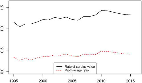
where is the total wage of the productive sectors. While the exploitation rate expressed in equation (2) is identical to the aggregate profit–wage ratio, the one in equation (4) is not, since the wage in the unproductive sectors is counted in the numerator of the exploitation rate and the labour share of the mixed income is added to the denominator. Therefore, the overall trends of the two ratios are usually different from each other in the case of the US economy as shown in Shaikh and Tonak (1994). In the case of the Korean economy, Figure 6 demonstrates that both the exploitation rate and the profit–wage ratio experienced an upward trend while the gap between the two has grown over time.

Figure 6. Rate of surplus value and profit–wage ratio, 1995–2015

Note: The numerator of the profit–wage ratio is measured by operating surplus including income receipt on assets from the rest of the world minus the labour income of the self-employed, while the denominator is measured by employment compensation including wage and salary receipt from the rest of the world plus the labour income of the self-employed.

By the same logic, the value of labour power in equation (3) is now replaced by:

(5)

The value of labour power measured accordingly is illustrated in Figure 7. It underwent a precipitous fall during the two crisis episodes, in 1997–1998 and 2008. While it seems to have been reversing the course in recent years since 2010, it has not recovered its pre-crisis level.

Figure 7. The value of labour power, 1995–2015

When the productive–unproductive labour is explicitly considered, as in this article, a discrepancy between the value of labour power and the labour share of national income emerges, which is in contrast to the definition in equation (3), where there is no such discrepancy. As the value of labour power is computed in relation to the total wage of the productive labours only, instead of the total wage of the whole labours, the value of labour power is necessarily smaller than the labour share of income. To see this formally, let us denote the labour share by LS, which then can be expressed as, by definition,

(6)

Combining equations (5) and (6) yields:

(7)

which conforms to that VLP < LS holds and, moreover, that their difference depends on the relative volume of total wage between the productive and unproductive sectors, that is, W_U/W_P.

Figure 8 compares the developments of the value of labour power and the labour share in income.¹⁰ While their secular trends are similar to each other, the value of labour power declined at a faster rate than the labour share did in the aftermath of the 1997–1998 crisis; after the early 2000s, the pace of the decline reversed, the labour share now falling more rapidly than the value of labour power. Interestingly, as shown in Figure 9(a), the share of value added of the unproductive sectors constantly increased until the mid-2000s, but stabilised afterwards.

Figure 8. The value of labour power and the labour share in income, 1995–2015 (1995=1).

Figure 9. The share of unproductive sectors, 1995–2015

The results in Figures 8 and 9(a) together indicate that exploitation in the unproductive sectors intensified after early 2000s.¹¹ This is because when the nominal value added of the unproductive sectors increased and, later, stagnated – as shown in Figure 9 (a) – the fact that the labour share fell more than the value of labour power did after the early 2000s – as displayed in Figure 8 – implies that, according to equation (7) W_U/W_P decreased during this period; it is a short step from the rise in the share of the value added of the unproductive sectors and the decline in W_U/W_P to deriving a rise in the profit–wage ratio of the unproductive sectors.¹²

In fact, our data demonstrate that exploitation in the unproductive sectors has intensified throughout the entire sample period. On the one hand, Figure 9(b) charts the share of unproductive activities in terms of employment and compensation. It is readily observed that the share of total employment of the unproductive sectors is rising whereas the share of their total wages is falling albeit rather slowly. The combination of these two trajectories confirms that exploitation in the unproductive industries strengthened throughout the sample period. On the other hand, Figure 10 more clearly and directly shows that the labour share of the unproductive industries went through a sharp decline in the immediate aftermath of the 1997–1998 crisis and has continue the downward trend thereafter.

Figure 10. Labour share in income of unproductive sectors, 1995–2015

The increase in the share of unproductive activities in Korea – as evidenced in Figures 9(a), 9(b) and 10 – corresponds to the experience of other developed capitalist economies; for the case of the US economy (see, for example, Paitaridis and Tsoulfidis 2012; Basu and Foley 2013).¹³ Notice that Marxian economic theory considers the expansion of unproductive activities as a threat to capital accumulation (Shaikh and Tonak 1994; Paitaridis and Tsoulfidis 2012). In the case of the Korean economy, however, the expansion of unproductive activities does not seem to have undermined the conditions for capital accumulation as it took place along with the strengthening of exploitation in the unproductive sectors, which might have offset the negative effects of the expansion of the unproductive activities.

Lastly, examining the dynamics of the three key variables reported thus far suggests that our sample period can be divided into two sub-periods in the same way as in Table 1. The average annual rates of change of the value of labour power and the rate of exploitation during 1996–2010 and 2011–2015 are summarised in Table 2. The period of 1996–2010 is characterised by a rise in the rate of exploitation and a decline in the value of labour power and the labour share, whereas these trends are all reversed during the period of 2011–2015. Tables 1 and 2 put together suggest that there is a structural break in our sample period before and after around 2010–2011.

Table 2. The annual rate of change of the value of labour power and the rate of exploitation (%)

	Exploitation rate	Value of labour power	Labour share
1996–2010	1.53	-0.56	-0.68
2011–2015	-1.46	0.96	1.03

Marxian Value Analysis: Sectoral Level

We now plot the Marxian ratios at the industry level, aiming to gain a more concrete understanding of how the performance of manufacturing has related to the overall condition of capital accumulation in the Korean economy. We measure the MELT and the rate of exploitation at the industry level. They describe two different dimensions of class conflict. The former reveals the inter-industrial distribution of value whereas the latter describes the capital–labour distribution of value in each industry.

Two methodological comments are required before proceeding. First, as the MELT is measured by national account data, our estimation of the industry-level MELTs reflects the end result of distribution of value among industries. That is, it illustrates realisation, rather than production, of value in each industry. Therefore, an inverse transformation from price variables to value variables is required for estimating the sectoral rates of surplus value. Second, since it is only the productive sectors that produce value and surplus value while the source of income generated in unproductive sectors is the value transfer from the productive sectors, our measures of the MELT and the rate of surplus value at the industry level focus on the productive sectors only.

Sectoral Monetary Expression of Labour Time

The MELT defined at the industrial level, denoted by m_i, is expressed as:

(8)

where MVA_i and L_i are money value added and total labour time of productive industry i.

In interpreting the relation between m_i and m, we rely on Okishio (1956), where the concept of “rate of income,” defined as income per unit of direct labour, is introduced and used in analysing the inter-industry value transfer; note that Okishio’s rate of income is conceptually identical to the MELT. To be more specific, Okishio took the ratio between, using our terminology, the MELT of the individual industry and the aggregate MELT, that is, , as an index of unequal exchange among industries and interpreted the ratio greater than one as implying gains from exchange while the ratio less than one as implying losses from exchange.

When the productive–unproductive labour distinction is taken into account, as in this article, however, we need to consider that is much more likely than not for most of the productive sectors since there is a systematic value transfer to the unproductive sectors, which do not produce value at all. In this sense, examining relative levels and overall trends of for the productive industries is more relevant when interpreting the relation between and , rather than asking whether the ratio is greater or less than one. Accordingly, we consider an increase (a decrease) in as implying that industry ’s position in the inter-industrial value transfer is enhancing (weakening) and the conditions for industry ’s capital accumulation in terms of both production and exchange are improving (deteriorating).

In this context, Figure 11 compares the relative trends of for the productive industries. While the absolute levels are not reported here, most productive industries displayed as expected. Exceptions are utilities and information services where the industry’s MELT is larger than the average and hence . One possible explanation is that these industries are characterised by natural monopoly; such industries are protected by entry barrier from the competitive force of profit rate equalisation through the process of surplus value distribution. They have a market power of price control, which enables them to achieve a higher-than-average level of MELT.¹⁴

The most interesting observation in Figure 11 concerns manufacturing. It uniquely exhibited a clear upward trend since the 1997–1998 crisis and a clear downward trend since 2011. That is, manufacturing was the only sector that experienced a persistent improvement in the conditions for capital accumulation during the long period stretching from the beginning of the sample period through around 2010. It is also the only sector that has gone through a persistent deterioration of the conditions for capital accumulation from 2011 until recent years.

Figure 11. of productive industries (1995=1)

In addition, the ratio can also be used to estimate the value transfer from the productive to unproductive sectors. To show this, let us first define the weighted average of m_i with the share of labour time of each industry as the weight and denote it by m*. Then, we have:

(9)

Where ,, with i’s being productive industries. Next, note that there is a discrepancy between MVA_i and money value actually produced by industry i due to value transfer and unequal exchange vis-à-vis the other productive and unproductive industries. If we define , with i’s being productive industries, to denote the total money value added of the productive industries as a whole, MVA - MVA_P >0 represents the magnitude of the value transfer.

Furthermore, it can be easily verified that

(10)

holds. Then, the difference between the aggregate MELT, and the weighted average of the productive industries, estimates the value per labour time transferred from productive to unproductive sectors; that is,

(11)

Figure 12 charts historical evolutions of m and m* together. It is not only confirmed that m > m* holds; it is also clearly observed that the magnitude of the value transfer per labour time, indicated by the gap between the two trajectories, has steadily increased throughout the entire sample period. This is another indication of the expansion of unproductive activities in Korea that corresponds to the observations reported in Figure 9.

Figure 12. The monetary expression of labour time: the economy versus the aggregate productive sector, 1995-2015

Sectoral Rates of Exploitation

Theoretical background

The conventional assumption in Marxian economics that the sectoral rates of exploitation converge to the average implies perfect competition in labour markets. While this can be useful for a theoretical purpose as in the case of transformation of value into price of production, it is unrealistic to adopt the assumption when dealing with data consisting of actual market prices (see Rieu 2008, on related theoretical issues). Prevailing observations about huge differences in working conditions depending on workers’ education, skills and the like make it unrealistic to assume that the conditions of exploitation tend to be equalised over time. For this reason, the central hypothesis in this section is that there is no tendency for the sectoral rates of exploitation to converge to a unique value.

In order to verify whether there is any empirical support to our hypothesis, we conducted panel unit root tests on the time series of the deviation of the sectoral rate of exploitation from the mean. We used two different Augmented Dicky-Fuller tests proposed by Im, Pesaran, and Yongcheol (2003) and Maddala and Wu (1999), respectively. For both tests, the null hypothesis is that a unit root is present in all the time series, whereas the alternative hypothesis is that there is no unit root in some of the time series. The fact that the time series of the deviation do not have a unit root and hence are stationary implies that the deviations do not develop permanently but are corrected by reverting to the mean. In contrast, the presence of a unit root implies that the time series of the deviation are non-stationary and thus do not exhibit mean reversion. Therefore, if the null is not rejected, we can safely discard the assumption of the equalisation of the sectoral rates of exploitation.

The test results are reported in Table 3. The validity of our hypothesis depends on the model specifications. At the significance level of 5%, the p-value larger than 0.05 can be taken as implying the presence of unit roots. Except for the model with a time trend, the results suggest either moderately – in the case of the model without a time trend – or strongly – in the case of the model without a drift and a time trend – that our data do not display an equalisation of the sectoral rates of exploitation. We conclude that imposing the equality of the sectoral rates of exploitation would not fit well, at least, to the case of the Korean economy during 1995–2015.¹⁵

Table 3. Panel unit root tests on the rate of exploitation at the industry level: p-values

	Im, Pearson, and Shin test	Maddala and Wu test
Model without a drift and a time trend	n.a.	0.164
Model without a time trend	0.643	0.728
Model with a time trend	0.024	0.025

The novel approach we propose relies on the inverse transformation of a price variable to a value variable. That is, instead of directly computing the sectoral rates of exploitation, we first obtain the labour share at the industry level and from the latter derive the sectoral rates of exploitation. Similarly to the case of measuring the labour share of the whole economy, we decompose the income of the self-employed of each industry into capital income and labour income according to the profit–wage ratio of the industry in question, as discussed above. One of the problems in doing this is that the income data of the self-employed are available only at the aggregate level rather than industry level. In addressing this issue, we follow the Jeon and Joo (2015) method to distribute the total income of the self-employed sector to each individual industry by taking the wage differentials among the industries into consideration. Thus distributed, the income of the self-employed in each industry is then decomposed into capital income and labour income according to the profit–wage ratio of the industry.

Next we present the theoretical relation of the inverse transformation between the exploitation rate and the labour share in income at the industry level. Let us denote the labour share in income of industry i by LS_i and its value equivalent by LS_i^VALUE. On the one hand, LS_i^VALUE is, by definition,

(12)

where V_i, S_i, and e_i are variable capital, surplus value and exploitation rate in industry i, respectively. According to the NI, the exploitation rate of industry i can be computed as follows:

(13)

where w_i denotes the wage rate in industry i (for the derivation see Rieu 2008). Equation (13) holds under the assumption that the value-creating capacity of the aggregate labour in each industry is the same.¹⁶ Combining equations (12) and (13) yields, on the one hand:

(14)

On the other hand, LS_i can be expressed as:

(15)

where m_i is the MELT in industry i, that is, the ratio between value added and labour time defined in industry i. From equations (14) and (15), we obtain:

(16)

which, when combined with equation (12), generates:

(17)

Equation (17) demonstrates the relation of inverse transformation and accordingly enables deriving e_i when LS_i is given along with m and m_i.

Furthermore, note that the profit–wage ratio in industry i corresponds to its exploitation rate in price terms; when the ratio is denoted by which can be expressed as

(18)

From equations (17) and (18), the following relations can be obtained:

(19)

It states that the deviation between m and m_i, which reflects inter-industrial value transfer and unequal exchange, is related to the deviation between the sectoral exploitation rate and profit–wage ratio, which reflects the capital–labour distribution of value. In this instance, m > m_i (m < m_i) indicates that the exploitation is more (less) intense than when it is measured by the labour share of income.

Estimation

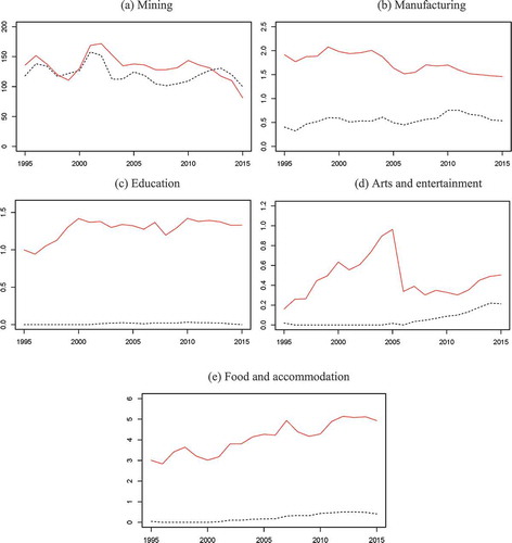
In relation to the inequalities in equation (19), we report the rate of exploitation e_i and the profit–wage ratio at the industry level in Figure 13. As expected, it is clearly noticeable that manufacturing has uniquely experienced the gap between the exploitation rate and the profit–wage ratio getting shrunk until 2011, which implies a steady rise of m_i/m according to the relation in equation (19); it is also observable that the gap has started to increase thereafter, implying a decline of m_i/m. This result exactly corresponds to the dynamics of m_i/m of manufacturing as displayed in Figure 11. In all, the figure demonstrates that while manufacturing has exhibited an upward secular trend of the profit–wage ratio and a downward secular trend of the exploitation rate, its position in relation to the other productive and unproductive industries steadily improved until 2011, after which it has started to get undermined.

Figure 13. The exploitation rate and the profit–wage ratio at the industry level, 1995–2015

We have also estimated the exploitation rates and the profit–wage ratios for manufacturing at two-digit industry level and reported in Figure 14 the results for three major manufacturing industries – electrical and electronic products, petroleum, coal, and chemical manufacturing and transportation equipment. Note that the share of these three major manufacturing industries in total manufacturing is, at an annual average, 65.6%, which rises to 83% when metals is included.

Figure 14. The exploitation rates and the profit–wage ratios of manufacturing at two–digit industry level, 1995–2015

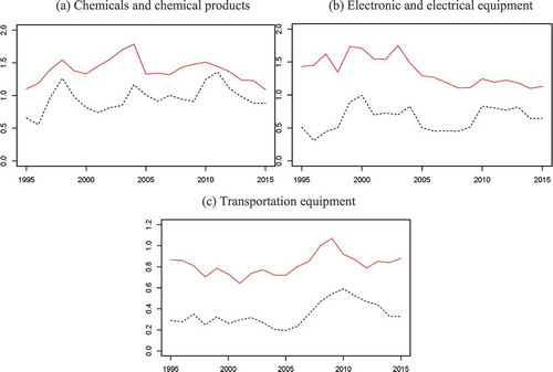
The overall trend of electrics and electronics and that of coal, mining, and chemicals seems to be the driver of the behaviour of the entire manufacturing sector as they exhibit similar shapes. In the case of transportation, however, it is somehow different. These three manufacturing industries have the largest MELT among the entire manufacturing industry and are marked by a declining trend in recent years after 2011. Six out of eleven manufacturing industries with the MELT larger than the average, m*, of the productive industries are collected in Figure 15.

Figure 15. The monetary expression of labor time: manufacturing at two–digit industry level, 1995–2015

One of the important results that emerges from the estimates of sectoral exploitation rates in Figures 13 and Figure 14 in relation to our analyses above has to do with the performance of manufacturing; it witnessed a long stretch of improvement in its conditions for capital accumulation amid the expansion of unproductive sectors and the consequent rise in value transfer to the latter; this continued until 2011, after which the course has reversed.

We may relate these observations with the fact that for about a decade following the 1997–1998 crisis, export of manufacturing maintained a stable rise with the help of favourable conditions in the global economy. For example, the manufacturing industry recorded a 10.38% sales growth rate during this ten-year period, which however was lowered to -0.07% after 2010 due to the global recession. Whether this structural change can be explained by the fact that the export-led growth regime has been dismantled as Uni (2017) and Palley (2011) suggest is a question that requires further investigation. See, for instance, Figure 16 which displays exchange rates, one of the crucial conditions for an export-led growth regime. The Korean Won, after the sharp spike during the 1997–1998 crisis episode, underwent a long period of gradual appreciation against the US dollar.

Figure 16. Foreign exchange rates, 1995–2015

Conclusion

Neo-liberal structuration since the 1997–1998 Asian economic crisis has made the forces of globalisation more influential within the Korean economy. In this article, we examined the Korean economy through the perspective of Marxian value theory. In order to understand the changing conditions for capital accumulation, we focused on class analysis and inter-sectoral value transfer by estimating the sectoral rates of exploitation along with the sectoral MELTs. One of the novelties of this article is to explicitly consider the self-employed sector, the weight of which is uniquely high in the Korean economy, and decompose its income into capital income and labour income when measuring the sectoral rates of exploitation. Some of the key results of this article are summarised as follows.

First, the value transfer from the productive industries to the unproductive industries steadily increased after the 1997–1998 crisis up until the mid-2000s. At the same time, however, exploitation in unproductive industries markedly intensified, particularly so in the immediate aftermath of the 1997–1998 crisis. The combination of these two opposing tendencies of capital accumulation may explain the fact that the conditions for capital accumulation were not significantly undermined in Korea during 1995–2015 when the unproductive activities steadily expanded.

The second finding has to do with the uniqueness of manufacturing in the capital accumulation in the Korean economy. Manufacturing maintained a consistently high level of the rate of exploitation during most of the period but experienced a decreasing trend at around the mid-2000s. Its MELT was on a steady rise until 2011, after which it started to fall. More importantly, manufacturing was the only productive industry that witnessed a fall in the value transfer to other industries until around 2010; then afterwards, again, it was the only productive industry where the value transfer increased. It can be concluded that the condition for manufacturing’s capital accumulation steadily improved from the 1997–1998 crisis, but started to deteriorate after 2011.

Factors associated with globalisation such as moving factories overseas might have been crucial for the improvement of the conditions for capital accumulation of manufacturing achieved amidst the steady rise in the unproductive sectors. However, the conditions for export-led growth have started to collapse since 2010, and the Korean economy has thereafter entered a conjuncture that requires a regime change towards domestic demand-led growth. Our value-theoretic analysis provides a foundation for understanding the context of the regime change, which may plausibly characterise the Korean economy’s last couple of decades.

Acknowledgments

The authors are grateful to Sangyong Joo and Su Min Jeon for generously providing the data on the labour income share of Korea. This study would have been impossible without their support. We also thank Jonathan F. Cogliano, Jeong Joo Kim, Xiao Jiang, Fred Moseley, Naoki Yoshihara, Jayoung Yoon, two anonymous referees, and participants at the 2018 Winter Conference of the Korean Association for Political Economy in Seoul and the 2018 Annual Meeting of the Eastern Economic Association in Boston for useful comments and suggestions. The usual caveat applies.

Disclosure Statement

No potential conflict of interest was reported by the authors.

Notes

1. This is one of the advantages of the NI over the other interpretations of Marxian value theory and the main reason why we adopt it as a framework for the empirical analysis in this article. We recognise that there is a critique of the NI that it explains values from prices rather than the other way around and thus that “the whole relation between surplus value and profit is turned on its head” (Shaikh and Tonak 1994, 179). However, this view is misdirected since in the NI the labour value categories are not determined by, but recovered from, the price categories.

2. Jeong and Jeong (2020), which appears in this special issue, differs from ours in two ways. First, their methodology in distinguishing between productive and unproductive labour is more sophisticated, relying upon the input–output table. Second, in their article, an estimation of the rate of profit and the rate of surplus value is based on a more traditional approach; for instance, the value of labour power is still interpreted in connection to the value of means of consumption. The result is that their empirical results are somewhat different from ours.

3. Sources of the data used in the article are explained in the appendix and details of estimations are found in the note of each figure.

4. Two points should be observed. First, we computed the capital share of national income by following Joo and Jeon’s (2014) method, that is, to decompose the operating surplus of self-employed, unincorporated sector – which is officially categorised as capital income – into capital income and labour income according to the profit–wage ratio of the corporate sector. Second, the measure of the profit rate in Figure 2 assumes away the distinction between productive and unproductive labour. When the distinction is taken into consideration, however, the wage of unproductive industries will need to be added to the numerator of the profit rate as part of total surplus value. We will start to incorporate the productive–unproductive labour distinction into our analysis from the next section.

5. In Hong (2013), the manufacturing industry’s output–capital ratio, which corresponds to our capital productivity, was in an upward trend from the 1997–1998 crisis to 2009. This difference can possibly be explained by the fact that Hong measures the ratio in real terms while we use nominal terms and that Hong uses value added while we use net national income.

6. The productive industries include agriculture, forestry and fishery, mining, manufacturing, utilities, construction, accommodation and food service, transportation and warehousing, information services, education service, arts and entertainment.

7. The underlying assumption is that the labour share in income is identical between the incorporated and unincorporated sectors.

8. See Mohun (2006) for a summary of the theoretical framework of the NI in the context of an empirical analysis.

9. While Ⓑ could be a useful approach in separating out the supervisory labour from the productive labour as shown in Sung (2007) and Jeong (2015), it is difficult to apply without some restrictive assumptions since the data published by the Ministry of Employment and Labour (2003–2017) is based on a sample inspection instead of a full and complete one.

10. In relation to the discussion of Piketty above, we can examine the behaviour of the value composition of capital (VCC) using K/W_P as a proxy. From the estimation, the result of which is omitted in this article, we have observed that for both the whole economy and manufacturing the VCC increased during the two crisis episodes and then stagnated after 2010. In particular, the rising trend has been weaker in manufacturing than in the whole economy.

11. Although value and surplus value are not produced in the unproductive industries, exploitation may take place therein, as Foley (1986, 122) states that exploitation “through the wage labor relation occurs when a worker expends more labor hours than he or she receives an equivalent for in wages.”

12. It should be noted, however, that this relation holds only under certain conditions.

13. Paitaridis and Tsoulfidis (2012) document the rise in the share of the unproductive sectors in terms of employment and wages whereas Basu and Foley (2013) focus on employment and value added. It should be noted, however, that Basu and Foley adopted the distinction between service and non-service sectors which is less controversial than the productive versus unproductive industry distinction.

14. For more discussions on the determinants of the sectoral MELTs, see Rieu, Lee, and Ahn (2014).

15. To our knowledge, Vaona (2011) is the only paper that precedes ours in using panel unit root tests to examine the hypothesis of equalisation of either the rate of profit or the rate of exploitation. As Vaona studies three European countries with a larger data set than ours, the Choi (2001) test, which is another available panel unit root test, is used in addition to the two tests we used; our data set is too small to employ the Choi (2001) test. The results reported in Vaona more strongly support the hypothesis that the sectoral rates of surplus value are not equalised.

16. The assumption of an equalised value-creating capacity of each industry’s aggregate labour is necessary in measuring the sectoral rates of exploitation from the real-world data. Duménil, Foley, and Lévy (2009) state that in “order to recover a measure of this value productivity from real-world price and wage data by sector, some additional assumption about relative rates of exploitation (which Marx often explicitly assumes to be equal) is required.” Hahn and Rieu (2017) present simulations that examine the consequence of the assumption that the value-creating capacity of the aggregate labour in each industry is not the same.

Appendix: Data Sources

The sources of the data used in this article are as follows:

• Assets, value added, and income used for computing Piketty’s β, income distribution, profit rates, capital productivity and the MELT come from National Accounts by Bank of Korea available at: https://ecos.bok.or.kr.

• Employment data used for computing income distribution and the MELT are obtained from Korean Statistical Information Service by Korea National Statistical Office available at: https://kosis.kr.

• Working hours data used for computing income distribution and the MELT are obtained from Survey Report on Labour Conditions by Employment Type published by Ministry of Employment and Labour (2003–2017).

References

- Basu, D., and D. Foley. 2013. “Dynamics of Output and Employment in the US Economy.” Cambridge Journal of Economics 37 (5): 1077–1106.
- Choi, I. 2001. “Unit Root Tests for Panel Data.” Journal of International Money and Finance 20 (2): 249–272.
- Cogliano, J. F. 2017. “Surplus Value Production and Realization in Marxian Theory – Applications to the U.S., 1987–2015.” Review of Political Economy 30 (4): 505–533.
- Duménil, G. 1980. De la valeur aux prix de production. Paris: Economica.
- Duménil, G., D. Foley, and D. Lévy. 2009. “A Note on the Formal Treatment of Exploitation in a Model with Heterogenous Labor.” Metroeconomica 60 (3): 560–567.
- Foley, D. 1982. “The Value of Money the Value of Labor Power and the Marxian Transformation Problem.” Review of Radical Political Economics 14 (2): 37–47.
- Foley, D. 1986. Understanding Capital: Marx’s Economic Theory. Cambridge, MA: Harvard University Press.
- Foley, D. 2013. “Rethinking Financial Capitalism and the ‘Information’ Economy.” Review of Radical Political Economics 45 (3): 257–268.
- Hahn, S, and D. Rieu. 2017. “Generalizing the New Interpretation of the Marxian Value Theory: A Simulation Analysis with Stochastic Profit Rate and Labor Heterogeneity.” Review of Political Economy 29 (4): 597–612.
- Hong, J. 2013. “The Rate of Profit of Korean Manufacturing.” [In Korean.] Marxism 21 10 (4): 10–44.
- Im, K, M. Pesaran, and S. Yongcheol. 2003. “Testing for Unit Roots in Heterogeneous Panels.” Journal of Econometrics 115 (1): 53–74.
- Jeon, S, and S. Joo. 2015. “Measuring Labor Income Shares at the Industry Level for Korea.” [In Korean.] Journal of Korea Development Economics Association 21 (4): 35–76.
- Jeong, G. 2015. “The Rate of Surplus Value in South Korea, 1980–2011: Improving the Weakness of Calculation Method Using ‘Monetary Expression of Labor Time’.” [In Korean.] Review of Social and Economic Studies (50): 25–58.
- Jeong, G., and S. Jeong. 2020. “Trends of Marxian Ratios in South Korea: 1980–2014.” Journal of Contemporary Asia 50 (2). DOI: 10.1080/00472336.2019.1643488.
- Joo, S., and S. Jeon. 2014. “Measuring Labor Income Share: Alternative Measure for Korea.” [In Korean.] Review of Social and Economics Studies 43: 31–65.
- Laibman, D. 1999. “Productive and Unproductive Labor: A Comment.” Review of Radical Political Economics 31 (2): 61–73.
- Maddala, G, and S. Wu. 1999. “A Comparative Study of Unit Root Tests with Panel Data and a New Simple Test.” Oxford Bulletin of Economics and Statistics 61 (S1): 631–652.
- Ministry of Employment and Labour. 2003 –2017. Survey Report on Labour Conditions by Employment Type. Seoul: Ministry of Employment and Labour. Accessed July 28, 2019, http://laborstat.moel.go.kr.
- Mohun, S. 2006. “Distributive Shares in the US Economy, 1964–2001.” Cambridge Journal of Economics 30 (3): 347–370.
- Okishio, N. 1956. “National Income and Labor.” [In Japanese.] Journal of National Economy 94 (4): 48–64.
- Oostveen, A., I. Biletta, A. Parent-Thirion, and G. Vermeylen. 2013. “Self-Employed or Not Self-Employed? Working Conditions of ‘Economically Dependent Workers’.” Dublin: European Foundation for the Improvement of Living and Working Conditions, EF1366.
- Paitaridis, D., and L. Tsoulfidis. 2012. “The Growth of Unproductive Activities, the Rate of Profit, and the Phase-Change of the U.S. Economy.” Review of Radical Political Economics 44 (2): 213–233.
- Palley, T. 2011. “The Rise and Fall of Export–led Growth.” Annandale-on-Hudson: Levy Economics Institute of Bard College, Working Paper No. 675.
- Piketty, T. 2014. Capital in the Twenty-First Century. Cambridge: The Belknap Press.
- Rieu, D.-M. 2008. “Estimating Sectoral Rates of Surplus Value: Methodological Issues.” Metroeconomica 59 (4): 557–573.
- Rieu, D, and S. Joo. 2014. “Marxian Ratios after Piketty.” [In Korean.] Review of Social and Economic Studies 45: 161–183.
- Rieu, D, K. Lee, and H. Ahn. 2014. “The Determination of the Monetary Expression of Concrete Labor Time under the Inconvertible Credit Money System.” Review of Radical Political Economics 46 (2): 190–198.
- Semieniuk, G. 2017. “Piketty’s Elasticity of Substitution: A Critique.” Review of Political Economy 29 (1): 64–79.
- Shaikh, A., and E. Tonak. 1994. Measuring the Wealth of Nations: The Political Economy of National Income. New York: Cambridge University Press.
- Sung, N. 2007. “Marx, Rate of Surplus-Value and the Technological Progress in Korea.” [In Korean.] The Korean Journal of Economic Studies 55 (1): 69–101.
- Uni, H. 2017. “The Transformation of Export-led Growth in East Asian Countries.” Paper, 14th International Karl Polanyi Conference, Seoul.
- Vaona, A. 2011. “Profit Rate Dynamics, Income Distribution, Structural and Technical Change in Denmark, Finland and Italy.” Structural Change and Economic Dynamics 22: 247–268.