The effect of school zone on housing prices: evidence from a quasi-natural experiment in New Zealand

Abstract

We analyse a quasi-experiment where a much sought-after state secondary school with no close substitutes unexpectedly reduced its enrolment zone twice over a three-year period. We use difference-in-differences to estimate the impact of the two downsizings on housing sales prices. We use controls for housing characteristics for pooled cross section or housing fixed effects for repeat sales, test for parallel trends, and conduct numerous robustness checks. In our main analysis, we find the first downsizing may decrease housing prices between 3.2% and 12.9%, with most estimates statistically significant, while the second downsizing may decrease prices between 2.1% and 7.2%, with most estimates insignificant. Tests in the pre-treatment period suggest parallel trends cannot be rejected, though some cross section interactions are significant when the two downsizings are analysed separately. We conclude the school zone’s first downsizing likely had a negative effect on housing prices of a small to moderate magnitude.

KEYWORDS:

• School housing price premium
• difference-in-differences
• hedonic house pricing models

I. Introduction

Many public education systems ration access to scarce public school spaces using school enrolment zones (OECD, 2019). Housing with access rights to desirable local public schools might be predicted to command higher sales prices than housing without, as access rights become capitalised into property values.

Alongside parents, education policymakers are often concerned with public school enrolment systems, seeking equitable access to high-quality education and the full use of existing school networks (Maguire, 2019). To encourage the uptake of less popular schools by local families, policy makers may seek to limit the zones or out-of-zone enrolments of more sought-after schools. Yet by using restrictive zone policies to pursue equity objectives, policymakers may inadvertently find housing prices bid up in sought-after zones, limiting access to such schools only to wealthier families. Thus, knowing the extent to which restrictive zoning affects the price of housing should be of relevance to both parents and policymakers.

In this paper, we estimate a housing price premium caused by access rights to a sought-after state school, by analysing how the market responded to two successive reductions in the enrolment zone of a popular high school in Christchurch, New Zealand. Cashmere High School (CHS) is a Decile 9 state school without close substitutes nearby, in a higher-income area in the south of the city. We employ a difference-in-differences (DID) approach to a hedonic house pricing model to compare the changes in housing prices before and after the two re-zonings, between houses remaining in-zone versus those excluded.

We find that compared to remaining in-zone, losing access in the first downsizing may have caused an average decrease in the price of between 3.2% and 12.9% in the following period. In contrast, we mostly find no significant price effect of the second downsizing. To the best of our knowledge, this is the first study to test school zone effects on housing prices in New Zealand using DID. More generally, an advantage of conducting this exercise in New Zealand is that the country’s state schools receive almost all of their funding centrally, rather than from local property taxes. This helps reduce endogeneity from the correlated socio-economic status of households in the relevant school’s zone.

The paper proceeds as follows. Section 2 reviews the literature regarding school quality and housing prices. Section 3 provides institutional information regarding school access in New Zealand and CHS. Section 4 describes our data and the difference-in-differences method. Section 5 provides our results and robustness checks, and Section 6 concludes.

2. Literature review

The most common way of estimating the effects of school access rights on housing prices has been hedonic pricing models, repeated sales models, and combinations of the two (Cho, 1996 and Malpezzi, 2003). Lancaster (1966) and later Rosen (1974) proposed hedonic pricing models to decompose the price of a comprehensive good into components by attaching an implicit price to each underlying attribute. Applied to housing, researchers could regress housing sales prices on-site and neighbourhood characteristics to estimate the marginal contribution of each attribute to the overall sales price. Later researchers have also regressed sales price on the attributes of spatially lagged properties weighted by distance (Goodman & Thibodeau, 2003), or on a property’s access to local amenities, and environmental attributes such as air or water quality.

In New Zealand, as reviewed by Fernandez (2019), most hedonic researchers have focussed on the price effects of environmental amenities (Bond, 2007; Plimmer, 2014; or Fleming, Grimes, Lebreton, Maré, & Nunns, 2018). Internationally, however, many hedonic studies have estimated the price effects of access to high-quality public schools.¹ Theoretically, Tiebout (1956) extended the Musgrave-Samuelson theory of public finance to local public goods, which predicts that better local schools should raise local demand for housing, creating a price premium. Undergirding the theory and empirical studies, parents are assumed to choose schools to maximize their children’s current satisfaction, but also to best invest in their future human capital. According to a 2009 survey in the OECD’s Programme for International Student Assessment (PISA), the top five factors parents consider when assessing school quality are academic achievement, reputation, pleasant environment, safety, and distance from home.² Belfield (2004) recognizes that parents are also choosing between public, private (independent or religious), home schooling, or as in New Zealand, public/private hybrids called state-integrated schools. As Bifulco, Ladd, and Ross (2009) find, school zoning policies can affect parents’ residential location decisions, with knock-on effects regarding segregation of students by socio-economic status and parental education.

Researchers have measured school quality in various ways. Prior to the 1990s, researchers mainly used per-student expenditure at the school or district level (e.g. Oates, 1969; Hyman & Pasour, 1973; Rosen & Fullerton, 1977). Later researchers used output measures, such as grade-level test scores (Li & Brown, 1980; Jud & Watts, 1981) national standardized exam results, or state-level math exams (Black, 1999). Other output measures have included the number of graduates entering an elite university (Bae & Chung, 2013) or school ratings (Figlio & Page, 2003). Some have transformed student test scores into value-added measures by controlling for student prior achievement (Brasington, 1999; Gibbons, Machin, & Silva, 2013). However, some researchers still use input-based measures, such as student-teacher ratio (Card & Krueger, 1992) or peer effects (Wang, Yuan, Min, & Rozelle, 2021). Where researchers have compared measures for explaining variation in housing prices, output indicators generally outperform input indicators (Downes & Zabel, 2002; Crone, 2006; Seo & Simons, 2009).

Hedonic methods have improved over time. Early school effect studies tended to inadequately control for neighbourhood characteristics correlated with school quality, and used single-year cross-sectional analysis (Jud & Watts, 1981). Early studies also sometimes proxied for housing value using appraisal prices or insurance valuations (Oates, 1969; Atkinson & Crocker, 1987) or used small samples (Walden, 1990).

Subsequent studies moved to panel house fixed-effects models, or incorporated spatial autocorrelation. More recent studies have tried to strengthen causal identification, using instrumental variables, boundary discontinuities, difference-in-differences, or following education reform interventions.

For example, Black (1999) pioneered using boundary-fixed effects to estimate the impact of elementary school quality on housing prices, comparing houses on both sides of school district boundaries in suburbs of Boston. She avoids uncontrolled neighbourhood heterogeneity by only considering house sales within .15 miles of zone boundaries. Compared to previous studies, Black’s use of boundary-fixed effects reduced the estimated school effect to half its previous size; a standard deviation increase in school test scores was associated with a modest 2.1% increase in house prices. Brasington (1999) and Brasington and Haurin (2006) initially include distance to the CBD, and advance to include spatial autocorrelation. Ries and Somerville (2010) find significant effects of secondary school quality on housing prices in Vancouver Canada. They use a DID method, trying both cross-sectional hedonic regressions and repeat sales analysis. Similar DID analysis has since been applied by Haisken-DeNew, Hasan, Jha, and Sinning (2018), Wen, Xiao, and Zhang (2017), Huang, He, Xu, and Zhu (2020), and Han, Shen, and Zhao (2021), often using quasi-natural experiments of education policy changes. We follow this latter approach.

In results, most recent research has found that access rights to high-performing schools have a positive effect on housing prices (see for example Barrow, 2002; Figlio & Lucas, 2004; and Bayer, Ferreira, & McMillan, 2007). Using a 10-year dataset of 8^th-grade math scores in Connecticut, Clapp, Nanda, and Ross (2008) find a standard deviation increase in scores raises housing prices by 1.3-1.4%. Dougherty et al. (2009) find that, after controlling for neighbourhood, proximity to attendance boundary, and student minorities, house purchasers are willing to pay a 1.9% higher price per standard deviation increase in test scores.

Researchers in Europe have also found positive effects of access rights on housing prices, with average effect sizes between 2 and 7 percent per standard deviation increase in school quality measure (Gibbons & Machin, 2006; Brasington & Haurin, 2006; Fack & Grenet, 2010; and Davidoff & Leigh, 2008). Relevant here, Machin and Salvanes (2007) find for Oslo Norway that prices adjacent to high-quality schools (based on secondary test scores) fell by 2-4 percent when access changed from zone-based to open enrolment. At the upper end, Leech and Campos (2003) find a 16–20 percent price premium for access rights to two elite secondary schools in Coventry, UK. Conversely, Brehm, Imberman, and Naretta (2017) find changes in access rights to charter schools do not affect house prices in Los Angeles County between 2008 and 2011.

Survey papers and meta-analyses have also been conducted. Nguyen-Hoang and Yinger (2011) surveyed 50 studies covering 1999 to 2010, while Black and Machin (2011) surveyed 54 covering a wider time span. Considering both together, fewer than five papers find no effect or non-conclusive results, and the vast majority find a positive association between school quality and house price. In meta analyses, Turnbull and Zheng (2021) conclude based on 56 papers that the choice of school quality measures is a key cause for the literatures’ mixed findings regarding effect size. Peer effect or value-added test scores show lower levels of effect compared to other output- or input-based measures. Turnbull and Zheng also find that region matters, with school quality price effects weaker in the southern United States than its other regions. Interestingly, by comparing results from boundary vs. neighbourhood fixed effects, the authors find that econometric methods do not appear to be driving results. However, greater control for neighbourhood amenities consistently reduces the size of effect.

Yadavalli and Florax (2013) also carry out a meta-analysis of 48 United States-based studies. They find elementary or high school test scores and expenditures per pupil in particular have significant effects on house prices.³ While Yadavalli and Florax find these measures significant, the direction and magnitude of effect are not conclusive. They attribute this to the underlying studies being mis-specified, or to the inclusion of multiple school quality measures complicating model interpretation.

Finally, Zhang et al. (2020) synthesize 38 Chinese studies from 2006 to 2017 and find using random effects meta regression that the effect of school quality is higher in compulsory years (Years 1-9) than non-compulsory (Years 10-12). They also find adjacency to zone boundary has a significant impact on price effects. Zhang et al. conclude that heterogeneity in individual city housing markets and the distribution of schools in each city accounts for the differences in size of price effects across studies, as individual studies typically focus on one city.

Investigations of school effects on housing price in New Zealand are far more limited, though the topic elicits media interest (Wilkes, 2020). Media reports tend to exaggerate school access price premiums, for example by comparing mean housing prices in a sought-after school zone with that for the rest of a city (Edmunds, 2017). Ignoring that other desirable neighbourhood characteristics likely co-vary with good schools have resulted in premiums estimated between 1% and 90.5%.

We have found four NZ-focused academic papers. McClay and Harrison (2003) use simple OLS regressions to estimate the price premium of housing being in Christchurch Girls’ High School zone using sales data for 514 houses in Christchurch. They find the in-zone premium could be as high as $203,000, or 53 percent of mean sale price. Using similar data but including spatial lags, Gibson, Sabel, Boe-Gibson, and Kim (2005) find the same premium falls to $77,000. As with McClay and Harrison, however, Gibson et al. omit controls for environmental and other public amenities. Rehm and Filippova (2008) use a larger dataset from downtown Auckland. Using suburb dummies in their hedonic models, they find that price premiums at the periphery of a desirable school zone are diminished, perhaps due to uncertainty regarding future boundary changes.

Finally, Gibson and Boe-Gibson (2014) re-estimate price effects using high school NCEA achievement rates (qualification achievement rates at several levels) and a 12-month sales dataset in Christchurch. They find a standard deviation increase in Level 1 NCEA achievement rate is associated with a 6.4% increase in housing price, controlling for spatial autocorrelation, housing characteristics, and neighbourhood demographic features.

3. Housing prices and zoning for cashmere high school

There are two major housing price indices in New Zealand: the Real Estate Institute of New Zealand's Housing Price Index (REINZ HPI) and the QV House Price Index. As of October 2021, the median New Zealand housing price was $890,500 according to REINZ, and $1,002,153 according to QV. Christchurch, with a relatively elastic supply of flat land for housing, has amongst the lowest median prices of the country’s major cities (NZ$668,000 in October 2020).

Turning to education, New Zealand’s pre-tertiary education system consists of thirteen years, divided into primary (Years 1–8) and secondary (Years 9–13). According to the Organisation for Economic Cooperation and Development (OECD), New Zealand has above-average education attainment and labour market outcomes compared to the rest of the world (OECD, 2021). The most recent Programme for International Student Assessment (PISA) results indicate that New Zealand students have higher performance in reading, mathematics, and science compared to the average of OECD countries, though with recent declines (Schleicher, 2019).

In New Zealand, parents can choose among state, state-integrated, and private schools, as well as home-schooling. State schools are fully state-owned and funded, whereas integrated schools are partially state-funded, with a special character. As of July 2020, the share of students going to state, integrated, and private schools, or being home-schooled, were 84%, 10%, 5% and 1%, respectively.⁴

New Zealand’s Education and Training Act 2020 (S33(1)) requires that ‘[e]very domestic student is entitled to free enrolment at any state school … .’ To implement this, the Ministry of Education (Ministry) can develop enrolment zones for popular schools with the potential for overcrowding, and criteria by which schools may accept out-of-zone applicants. This is justified as ensuring a fair and transparent enrolment selection process where necessary and optimizing the use of the existing network of state schools (Education and Training Act, 2020, S71.1). Schools with a zone must define their geographic areas, and children who live within a zone are entitled to enrol. If a school with a zone has excess capacity, it can offer places to out-of-zone students in a lexicographic order of priority, e.g. siblings of current and previous students have priority over other applicants. Within each ‘priority level’, if demand exceeds available places, selection takes place through a ballot (Schedule 20.3 Education and Training Act, 2020). Thus, to guarantee access to a specific school, parents must reside within its zone. But parents outside the zone may be able to enrol their child in a ballot if excess capacity exists.

The earliest enrolment zones were set up in 1999. By 2020, of 1484 state and integrated schools, 1075 had zones (MoE, 2021). Most of the schools with zones are adjacent to schools who also have zones, suggesting excess demand for state schools is spatially positively correlated.

The Ministry can react to uneven growth in schools by creating or modifying zones, adding classrooms to in-demand schools, or building new schools (MoE, 2019). Since 1999, the Ministry has gradually taken more control of zones from the boards of trustees of individual schools, over such issues as determining excess capacity that can be made available via ballots. This increased intervention has been justified on the basis of achieving more equitable access to schools across racial and socio-economic divides (Wilkes, 2020), though it also increases uptake at less popular state schools. Relevant for home-buyer expectations, this has resulted in a recent increase in once-rare adjustments to enrolment schemes for established schools, which can take parents by surprise. By the period 2018–2020, almost 5 percent of schools had changes implemented in their zones, according to the Ministry’s Enrolment Scheme Master data tool. At the local level, CHS’s enrolment scheme was introduced in 2004 and did not change until 2018.

3.1. Assessing school quality in New Zealand

There are three readily available quantitative signals that New Zealand parents can consult regarding school quality. Since the 1990s the Ministry has assigned each state and integrated school a decile rank from 1 to 10 based on five measures of the socio-economic disadvantage of the census meshblocks⁵ of its students’ families.⁶ While the Ministry created the decile system to target additional funding to schools with disadvantaged students, parents often treat higher decile ranking as a proxy for better school quality. As evidence, the number of students enrolled in Decile 6-10 schools grew continuously from 2013 to 2019, while falling at lower decile schools (Education Counts⁷).

The second quantitative signal of school quality is the qualification achievement rate of its students. New Zealand’s National Certificates of Educational Achievement (NCEA) are qualifications for students over the final three years of secondary school (Level 1 in Year 11 up to Level 3 in Year 13). General high school completion requires NCEA Level 2, while direct entry to university requires NCEA Level 3 or equivalent.

Thirdly, each school in New Zealand is periodically reviewed by the Education Review Office (ERO). While these reports are mostly qualitative, school inspectors take their holistic assessment into account in deciding how soon a school must next be inspected. Schools thought to be performing well are given the longest interval, six years.

3.2 Cashmere high school

Cashmere High School (CHS) is located next to the affluent southwest hills of Christchurch, the largest city on New Zealand’s South Island. Christchurch has 18 state or integrated secondary schools offering all year levels (Years 9-13), and 8 schools offering some.⁸ CHS is the city’s second-largest secondary school, with a roll of 1845 students as of July 2020.⁹

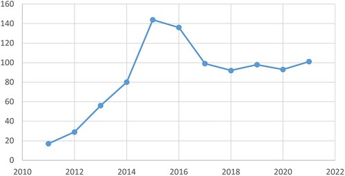
CHS is a Decile 9 school with a strong reputation, as evidenced by its consistently growing total enrolments between 2000 and 2020 (Figure 1) and Year 9 in-zone enrolments from 2012 to 2022 (Figure 2). The total number of out-of-zone applications to enrol for all year levels (not all successful) has also grown until 2015, though with some reduction since (Figure 3), possibly due to expectations of fewer spaces as spare capacity has decreased. The ERO's 2019 report states CHS. ‘consistently meets national expectations for at least 85% of students to leave with NCEA Level 2 or above’ (New Zealand Education Review Office, 2019). Its overall judgement was that CHS was ‘[w]ell placed’ in achieving valued outcomes for its students, and did not require another review for six years.

Figure 1. Number of total enrolments at CHS 2000-2020. Source: Education Counts.

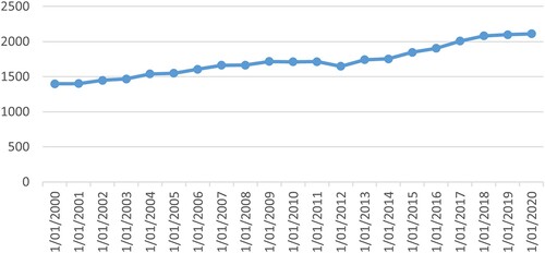
Figure 2. Number of year 9 in-zone enrolments at CHS 2012-2022. Source: Education Counts.

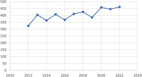
Figure 3. Number of out-of-zone applications at CHS 2011-2021. Source: Cashmere High School Office.

Unusually, CHS’s adjacent state or integrated schools have sharply lower decile ratings. These are Hillmorton High School (5.4 km distant, Decile 4), Linwood College (7.7 km distant, Decile 3), and integrated Hillview Christian School (3.9 km away, Decile 6), which only offers Years 9-10. This is our first evidence that alternative local schools would be unlikely to be perceived as close substitutes.

DID analysis requires careful attention to be paid to the dates at which parents or home-buyers became aware of zone downsizing. In October 2016, the Ministry commissioned KPMG to consult with the state secondary schools of Christchurch regarding the effectiveness of current enrolment zones. KPMG submitted a first report to the Ministry in April 2017, presenting six options for enrolment zone restructuring across the city, with pros and cons of each option, but without proposals for individual schools. In September 2017 the Ministry commissioned KPMG to create a follow on ‘Phase 2’ report proposing specific ‘Scenario T’ enrolment zone changes to reduce catchment demand for specific schools, including CHS.¹⁰ KPMP released the Phase 2 report to the Ministry in October 2017 (exact date not specified). This second report was not publicly released, so New Zealand media reported on it only on March 31^st 2018 after an official information act (OIA) request. In the mean time, CHS’s Board of Trustees proposed to the Ministry a different downsizing proposal in February 2018. The Ministry authorised CHS’s Trustees to proceed to seek downsizing on March 3^rd. A detailed comparison of two proposed downsizings was discussed in a three-party meeting among MoE, CHS’s Board, and KPMG’s analysts on March 28th. Key to our analysis, on April 4th the Board notified its feeder schools and community boards about its proposed changes and set a timeframe for public consultation. A public notice of the CHS proposal was printed in the local newspaper The Star on April 12th.¹¹ After incorporating minor changes, the Board’s proposal was approved by the Ministry on April 26th. A formal notice was issued by the Ministry on April 27^th, and the first downsizing came into effect on January 1st, 2019. As illustrated in Figure 4, those excluded were north-west of CHS, and re-assigned to Hilmorton High School (Decile 4). In our analysis, we will define this first area to lose access as Group A, and the second area (to be explained below) as Group B. Group C remains in the CHS zone throughout, while Group D is an adjacent area that was never in the zone.

Figure 4. Map of the first and second CHS zone changes. Source: This map is drawn according to the CHS school zone descriptions acquired from CHS website. See Appendix 1 for details.

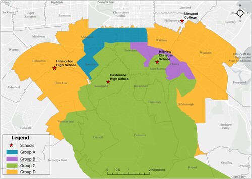
Perhaps because CHS or the Ministry did not anticipate that parents excluded from CHS’s zone would adjust by seeking properties within the remaining zone, the first downsizing did not sufficiently reduce in-zone admissions. As a result, on September 26^th 2019, roughly 17 months after the first downsizing was formally approved, CHS received a second official notification from the Ministry to further reduce its zone. More-so than the first, this second proposal aroused dramatic objection among local parents and homeowners. After the proposal was released for consultation on November 20^th, community meetings were held which attracted large turnouts. A typical complaint was that the excluded houses would drop in property value. Facebook groups were organized to challenge the new zoning, and a petition was submitted to Parliament, to no avail.¹² The second revision was publicly confirmed on April 17th, 2020, coming into effect on January 1st, 2021. Returning to Figure 4, those excluded in the second downsizing were north-east of CHS and re-assigned to Linwood College (Decile 3).

Aside from the differences in decile rankings with neighbouring schools already described, there are several strands of evidence that parents would view losing access rights to CHS unfavourably.

Linwood College’s 2020 ERO report states that ‘one third of students are leaving without attaining NCEA Level 2’ and its overall judgement of the school was ‘[d]eveloping.’ Follow-up evaluation was required in three years. The 2017 ERO report for Hillmorton High School was similar. Similarly, Tables 1 and 2 compare student retention rates and NCEA Level 1 achievement rates across the three schools, with noticeable gaps between CHS and the other two. In short, if ever one might expect to find a large effect of a change in school access rights on the price of housing, it would be from these downsizings.

Table 1. Comparison of student retention rates (2018–2020).

	Percentage staying until at least age 17
Comparison Groups	2018	2019	2020
Cashmere High School	89.1	88.2	89.3
Linwood College	63.7	68.6	64.5
Hillmorton High School	68.1	73.1	73.6
All Decile 04 Schools	79.3	77.8	78.7
All Decile 03 Schools	78.1	75.4	76.5
All New Zealand	83.8	82.8	83.5

Source: Education Counts, Ministry of Education, 2021.

Table 2. Comparison of NCEA Level 1 Achievement Rates (2018-2020).

	Percentage with at least NCEA level 1
Comparison Groups	2018	2019	2020
Cashmere High School	94.5	94.2	94.5
Linwood College	84.1	77.8	83.7
Hillmorton High School	80.6	77.1	82.2
All Decile 04 Schools	88.6	87.4	86.5
All Decile 03 Schools	86.3	83.6	83.8
All New Zealand	89.6	88.3	88.4

Source: Education Counts, Ministry of Education, 2021.

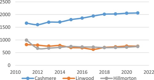
Before proceeding, we address a counter-argument that a large-scale transfer of students from CHS to adjacent schools could actually lessen differentials in outcomes, blunting any house price effects. We think this is unlikely. Figure 5 compares total student enrolments (net of international fee-paying students) across all three schools over the period 2011 to 2021. While the downsizings stalled growth in CHS enrolment, there is no evidence of a major corresponding boost in Hillmorton’s or Linwood College’s rolls since 2019. In fact, CHS’s slight increase in 2019 and 2020 might suggest excluded families have doggedly sought to purchase/rent housing in the remaining ‘Group C’ zone, which should augment any net price effects we subsequently find.

Figure 5. Student enrolment at Cashmere, Linwood and Hillmorton Schools. Source: Education Counts https://www.educationcounts.govt.nz/statistics/6028.

4. Data and empirical estimation strategy

The boundaries of CHS’s initial and updated enrolment zones were obtained from the school's official website and archived records from the Wayback Machine.¹³ We take the announcement dates by the CHS Board of Trustees (April 4th, 2018 and November 19^th, 2019) as our main cutoffs for the two changes in our main analysis. Effectively, we assume any effect on housing prices should start immediately after the announced zone revisions are publicly confirmed, well before the implementation dates. As a robustness check, in case CHS-specific recommendations from the Phase 2 KPMG report to the Ministry somehow leaked out, we also try excluding sales from October 1^st 2017 to April 4th 2018 from our analysis.

Data for housing sale prices and characteristics were acquired from CoreLogic (www.property-guru.co.nz), the authorized source of housing transaction data in New Zealand. We construct a dataset of all residential sales transactions by searching under ‘residential’, ‘anytime’ transactions from 26 suburbs in and around the initial CHS zone. The resulting dataset consists of 33,085 unique housing units. Linking house valuation reference number and profile, we scrape each house’s sales history to develop a dataset of 111,822 house-sale events.

Housing characteristics include Log House Price (transformed from Gross Sales Price), Suburb, Land Area, Floor Area, Building Age, Number Bedrooms, Number Garage, Outer Material, Roof Material, Contour (hilly or flat), Deck, and Sales Type (all or part of property). Characteristics also include Tenure Type, Sale Tenure, and bonafide, which we explain.

Tenure Type consists of: (1) single/whole sale, (2) multiple sale of two or more properties sold at once, (3) cross-reference sale where a property is sold together with a multiple sale transaction, and (4) only part of a property is sold. We use only the first because only there can we accurately identify the transaction price per property. Sale Tenure describes whether the property is (1) freehold with property and land, (2) leasehold with only property, (3) partial percentage share in property or (4) other. Again, we use only freehold sales to identify the value of the property as a whole. Finally, Bona Fide describes how arm’s length the transaction is: (1) an open market sale that can be roughly matched with estimated capital value, (2) an open market sale which cannot be roughly matched, and (3) a non-arm’s length sale, such as a gift or within-family sale. We exclude the latter two categories.

4.1 Data cleaning

Our first data cleaning involved dropping duplicate sales records, reducing housing sales from 111,822 to 90,870. For the few cases where housing sold multiple times in a year, we use only the last sale to maintain annual data, leaving 87,951 house sales. Following common practice in other hedonic studies, we next eliminated the few outlier sales prices higher than 2 million or lower than $100,000 NZD, and as described any non-freehold, non-whole, or non-bona-fide sales, as well as sales containing 0 sqm of floor area. This leaves 71,128 housing sales. Finally, as the housing market in Christchurch underwent tremendous damage and uneven development due to the 2010 and 2011 earthquakes, we exclude sales occurring before January 1^st 2012, creating a final dataset of 14,738 sales records from 11,093 unique houses between 2012 and 2021.¹⁴ As a robustness check, we later try excluding sales before 2015.

Some housing characteristics have missing values, particularly Number Garage. For pooled cross section regressions that control for such characteristics, our main approach for categorical variables is to create an additional ‘Unreported’ category. For continuous variables such as Number Bedrooms and Number Garage, we replace missing values with their sample means. As a robustness check however, we eliminate incomplete housing sales records, or also drop Number Garage.

4.2 Estimation strategy

In the simplest DID approach, we denote a single downsizing event with the binary variable $D_i\in \{0,1\}$. The outcome of interest is Log House Price, or $Y_i$. We want to know if being ‘treated’ (losing access) affects sales prices. If we assume that house i’s treatment status is randomly determined with no anticipation, the treatment effect ${\tau }_i$ is the difference (1) ${\tau }_i=(Y_i|D_i=1)-(Y_i|D_i=0)$(1) Since $Y_i$ is not observable both when $D_i$ = 1 and $D_i$ = 0, DID estimates an average treatment effect ${\tau }_{\mathrm{ATE}}$ by comparing the difference in group mean prices between the treated and control groups over the pre- and post-treatment periods, (2) ${\tau }_{\mathrm{ATE}}=E[Y_i|D_i=1]-E[Y_i|D_i=0]$(2) This can be denoted ${\tau }_{\mathrm{ATE}}=(\overline{y}{}_{T,2}-\overline{y}{}_{T,1})-(\overline{y}{}_{C,2}-\overline{y}{}_{C,1}),$ where T and C indicate treatment and control group, and 1 or 2 indicate pre- and post-treatment periods. Moving to a linear regression framework, the basic DID model is: (3) $Y_{\mathrm{it}}={\beta }_0+{\beta }_1.D_i+{\beta }_2.T_i+{\beta }_3.D_i\ast T_i+{\beta }_4.X_i+{\epsilon }_{\mathrm{it}}.$(3) Here $Y_{\mathrm{it}}\text{ is }$ the housing i sale price at time $t$; $D_i$ indicates whether i is treated (1) or not (0), and $T_i$ is pre-treatment period 0 or post-treatment period 1. $X_i$ is a vector of control variables. ${\beta }_1$ represents the price effect of being in the treated group area, while ${\beta }_2$ represents the effect of being in the post-treatment period. Of key interest, the coefficient ${\beta }_3$ on the interaction $D_i\ast T_i$ represent the average treatment effect on price of housing being assigned to group $D_1$. See Appendix 2 for additional detail.

To apply DID to more than one downsizing treatment applied in more than one area at more than one period, we extend to a j group, l treatment, k period specification: (4) $\begin{array}{rl}{Y}_{\mathrm{it}}& =\alpha +\sum _1^j{\beta }_j\mathrm{Grou}{p}_j+\sum _1^k{\gamma }_k\mathrm{Perio}{d}_k+\sum _1^l{\delta }_l\mathrm{Treatmen}{t}_l+\sum _1^j\sum _1^l{\phi }_{\mathrm{jl}}\mathrm{Grou}{p}_j\ast \mathrm{Treatmen}{t}_l\\ & +\sum _1^k\sum _1^l{\omega }_{\mathrm{kl}}\mathrm{Perio}{d}_k\ast \mathrm{Treatmen}{t}_l+\sum _1^j\sum _1^k{\rho }_{\mathrm{jk}}\mathrm{Grou}{p}_j\ast \mathrm{Perio}{d}_k\\ & +\sum _1^j\sum _1^k\sum _1^l{\pi }_{\mathrm{jkl}}\mathrm{Grou}{p}_j\ast \mathrm{Perio}{d}_k\ast \mathrm{Treatmen}{t}_l+{\epsilon }_{\mathrm{it}}\{i,t,j,k,l\}.\end{array}$(4) Here ${\beta }_j$ estimates the fixed effect of Group j on prices; ${\gamma }_k$ estimates the fixed effect of Period k on prices, and ${\delta }_l$ estimates the (time-invariant) fixed effect of downsizing event l as applied to some Group. Among single interaction terms, ${\phi }_{\mathrm{jl}}$ estimates the time-invariant effect of downsizing l for Group j; ${\omega }_{\mathrm{kl}}$ estimates the group-invariant effect of downsizing l in Period k, and ${\rho }_{\mathrm{jk}}$ estimates the (downsizing –invariant) fixed effect of Group j in Period k. The key coefficients of interest becomes ${\pi }_{\mathrm{jkl}},$ on the double interaction of downsizing l for Group j in Period k. Equation (4) can easily be augmented with $\sum _1^i{\theta }_i{X}_i$ control variables and $\sum _i^t{\eta }_t\mathrm{Yea}{r}_t$ fixed effects.

4.3 Assumptions of DID

The DID model assumes that all housing in the treatment group is treated simultaneously, with no anticipation prior to the treatment. The status of groups and periods also does not change over time. This systematic similarity between the treatment and the control groups is often called the ‘parallel trend’ assumption. Here, we assume that a downsizing treatment is independent of observed housing characteristics.

4.4 Identification

In our main approach, we assume any effect of losing guaranteed access to CHS starts immediately after each plan is publicly released by the CHS Board of Trustees (April 4^th, 2018, or November 19^th, 2019). This divides our timeline into three periods: t1 from January 1^st 2012 to April 4th, 2018, an intermediate period t2 between April 5^th, 2018, and November 19^th, 2019, and a final period t3 after November 19^th to the close of our data collection September 20^th, 2021. Because our first period extends over more years, for some specifications we add year dummies for 2012 to 2017, and a quarter dummy for the period January 1^st to April 4th of 2018 prior to the first downsizing announcement. We later try eliminating 2012 to 2014 sales, to make our three periods of roughly equal length.

Recall from Figure 4 that we define Group A as the first area to lose access, Group B as the second, Group C as always retaining access, and Group D as an adjacent area never in the zone. Applying our identification strategy, equation (4) will have j = 4 groups, k = 3 periods, and l = 2 downsizing treatments. Treatment events are defined as products: Treatment 1 = GroupA*t2, and Treatment 2 = GroupB*t3. We take Group C and Period t1 (and interactions involving them) as our omitted benchmarks. Adding year fixed effects and either housing characteristics $\sum _1^i{\theta }_i{X}_i\text{or }$ housing fixed effects $\sum _1^i{\theta }_i{H}_i$, equation (4) becomes: (5) $\begin{array}{rl}{Y}_{\mathrm{it}}& =\alpha +\sum _1^i{\theta }_i{X}_i+\sum _1^t{\eta }_t\mathrm{Yea}{r}_t+{\rho }_1\mathrm{GroupA}\ast t2+{\rho }_2\mathrm{GroupA}\ast t3+{\rho }_3\mathrm{GroupB}\ast t2\\ & +{\rho }_4\mathrm{GroupB}\ast t3+{\rho }_5\mathrm{GroupD}\ast t2+{\rho }_6\mathrm{GroupD}\ast t3+{\epsilon }_{\mathrm{it}}\end{array}$(5) Of particular interest is ${\rho }_1$ on the Group A*t2 interaction, and ${\rho }_3$ on the Group B*t3 interaction.

5. Main results and robustness checks

Not surprisingly given their differing sizes, Group C housing accounts for 44% of our total sales, Group D accounts for 36.7%, while Group A housing accounts for only 10.8%, and Group B 8.4%. Also not surprising given their unequal durations, there are fewer sales in t2 (16.9%) and t3 (14.9%) than in t1 (68.2%). Table 3 provides some descriptive statistics, while Figure 6 illustrates sales counts.

Figure 6. Comparison of sales counts by groups across periods.

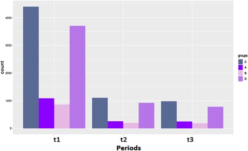
Table 3. Descriptive Statistics.

Variable Name	N	Percentage	Meaning
House ID	11093		ID of each unique house
Log House Prices	14738		Log of each house sales price
Groups	14738
-A	1598	10.8%	Houses losing CHS access in t1
-B	1236	8.4%	Houses losing CHS access in t2
-C	6492	44.0%	Houses staying within CHS zone all periods
-D	5412	36.7%	Houses never in CHS Zone
Periods	14738
-t1	10057	68.2%	From Jan 1st, 2012 to Apr 4th, 2018
-t2	2484	16.9%	From Apr 5th, 2018 to Nov 19th, 2019
-t3	2197	14.9%	From Nov 20th, 2019 to Sep. 20th, 2021
Year	14738
2012	1488	10.1%
2013	1611	10.9%
2014	1596	10.8%	Year of 2014
2015	1848	12.5%	Year of 2015
2016	1674	11.4%	Year of 2016
2017	1483	10.1%	Year of 2017
JanApr 2018	357	2.4%	From Jan 1st, 2018 to Apr 4th, 2018

For fixed effects analysis, what is especially relevant for precisely identifying treatment effects are the number of houses that sold both before and after the two downsizings, as illustrated in Table 4. Unfortunately, only 92 houses in Group A sold in both t1 and t2, and only 89 houses in Group B sold in (t1 + t2) and in t3. This may reduce the ability of fixed effects to precisely estimate the key interaction coefficients.

Table 4. Counts of repeat sales by group and period.

Identification		Count of Houses Sold in both pre & post periods
School Zone Changes	Pre Vs Post	A	B	C	D
1^st Downsizing	t1 Vs t2	92	78	418	367
	t1 Vs t2 + t3	203	155	782	706
2^nd Downsizing	t1 Vs t3	117	82	388	361
	t1 + t2 Vs t3	126	89	437	397
	t2 Vs t3	15	12	73	58

Also relevant for either fixed effects or pooled cross section are any systematic differences in housing prices between Groups, or over time, unrelated to CHS downsizing. The distribution of Log House Prices by group and period is illustrated using boxplots in Figure 7. Prior to downsizing, average sales prices tend to be higher in Group C than in the other three groups, and there is a slight upward trend in prices over periods. The boxplots also indicate there are more price outliers in Groups B and D than in A and C.

Figure 7. Boxplot of distribution of log house prices by groups and periods.

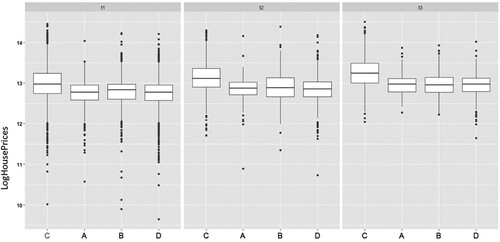
Figure 8 shows mean housing prices by group over time, and thus provides a first glimpse of potential treatment effects. Average price is consistently highest in Group C and lowest in D, but it also appears that price in Group A (and, oddly, in B) trend down in period t2 even as prices in C and D trend up. Meanwhile, all groups’ prices trend up in t3. Price drops in t2 for A may suggest a treatment effect, though the simultaneous lesser fall in B is puzzling.

Figure 8. Mean of loghouseprices of groups A, B, C, and D from 2012 to 2021.

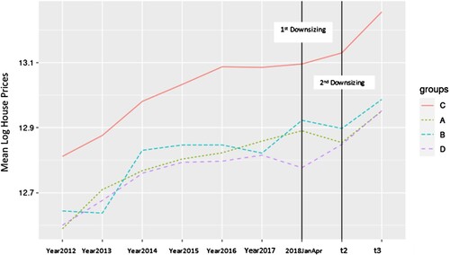
Table 5 next summarizes housing characteristics, relevant for pooled cross section analysis. The mean residence from our final sample has a floor area of 136 square meters, 2.9 bedrooms and 1.7 garage spaces, though with many missing values for the last of these.

Table 5. Summary of housing characteristics.

Panel (A) Continuous Variables
Variable Name	N	Mean	Standard Deviation	Min	Max
LogHousePrices	14738	12.911	0.398	9.649	14.502
FloorArea	14738	136	60.578	28	740
LandArea	10269	0.069	0.059	0.006	3.196
BedroomsNumber	14708	2.934	0.791	1	16
GarageNumber	3409	1.664	0.662	0	5
Panel (B) Discrete Variables
Variable Name	N	Percentage	Variable Name	N	Percentage
Contour of house site	14738		Building Age	14738
Level	7999	54.27	1880–1889	9	0.06
Easy to moderate fall	483	3.28	1890–1899	4	0.03
Easy to moderate rise	683	4.63	1900–1909	227	1.54
Steep fall	265	1.80	1910–1919	778	5.28
Steep rise	287	1.95	1920–1929	1227	8.33
NA – missing	5021	34.07	1930–1939	762	5.17
Deck	14738		1940–1949	725	4.92
Yes	4483	30.42	1950–1959	1130	7.67
No	4759	32.29	1960–1969	1317	8.94
NA – missing	5486	37.22	1970–1979	2005	13.60
Outer Wall Material			1980–1989	884	6.00
Brick	3813	25.87	1990–1999	1842	12.50
Weatherboard	3735	25.34	2000–2009	1683	11.42
Concrete	2875	19.51	2010–2019	1765	11.98
Roughcast, etc	2086	14.15	Mixed/Remodelled	93	0.63
Mixed Material	1472	9.99	NA – missing	287	1.95
Fibre Cement	425	2.88	Suburb	14738
Others	318	2.15	-Woolston	2214	15.02
NA – missing	14	0.09	-Spreydon	1793	12.17
Roof Material			-Hoon Hay	1572	10.67
Steel / G-Iron	9510	64.53	-Sydenham	1515	10.28
Tile	4815	32.67	-Somerfield	1403	9.52
Other	399	2.71	-Cashmere	1234	8.37
NA – missing	14	0.09	-Addington	1063	7.21
			-Waltham	817	5.54
			-SaintMartins	638	4.33
			-Westmorland	467	3.17
			-Hillsborough	448	3.04
			-Huntsbury	424	2.88
			-Beckenham	339	2.30
			-Opawa	270	1.83
			-Others proximate CHS	538	3.64

5.1 DID main results

Table 6 provides our main results. We begin with a basic version of equation (5) in Column (1), with neither housing characteristics nor housing fixed effects, but only group fixed effects. Column (2) adds controls for housing characteristics and year dummies within omitted period t1, with the quarter JanApr 2018 omitted. Column (3) replaces housing characteristics with housing fixed effects using the same omitted time and Group. Our treatment coefficients are GroupA*t2 and GroupB*t3.

Table 6. Empirical results.

	Column (1)	Column (2)	Column (3)	Column (4)	Column (5)
Dependent Variable:	Log House Prices
GroupA*t2	−0.048*	−0.073****	−0.092**	−0.138**	−0.032
	(0.028)	(0.021)	(0.042)	(0.057)	(0.130)
GroupB*t2	−0.032	−0.078***	0.003	−0.060	−0.049
	0.032	(0.024)	(0.045)	(0.063)	(0.120)
GroupD*t2	−0.039**	−0.054****	−0.003	0.007	0.069
	(0.018)	(0.014)	(0.026)	(0.034)	(0.067)
GroupA*t3	−0.077***	−0.061***	−0.118***	−0.125**	−0.061
	(0.029)	(0.022)	(0.038)	(0.057)	(0.128)
GroupB*t3	−0.068**	−0.075***	−0.021	−0.057	−0.0700
	(0.032)	(0.024)	(0.044)	(0.063)	(0.120)
GroupD*t3	−0.061***	−0.049****	−0.064**	0.012	0.005
	(0.019)	(0.015)	(0.026)	(0.034)	(0.067)
N:	14738	14738	14738	14738	14738
R^2	0.148	0.529	0.277	0.531	0.282
Adjusted R^2	0.148	0.526	−1.933	0.527	−1.93
F-Statistics
	233.2 on 11 and 14726 DF, p-value: < 2.2e-16	156.6 on 105 and 14632 DF, p-value: < 2.2e-16	99.545 on 14 and 3631 DF, p-value: < 2.22e-16	134.6 on 123 and 14614 DF, p-value: < 2.2e-16	44.274 on 32 and 3613 DF, p-value: < 2.22e-16
Fixed effects:
Groups	Y	N	N	N	N
Periods	Y	N	N	N	N
House ID	N	N	Y	N	Y
Years	N	Y	Y	Y	Y
House Features	N	Y	N	Y	N
Suburbs	N	Y	N	Y	N
Group T1 Year Interactions	N	N	N	Y	Y
Imputed Missing Values	N	Y	N	Y	N

Notes: 1. Standard errors in parentheses.

2. Significance levels: ‘****’ 0.001 ‘***’ 0.01 ‘**’ 0.05 ‘*’ 0.1

Consistent with our expectations, both interaction terms in Column (1) are negative and significant. Compared to houses in Group C in t1, prices in Group A decreased by 4.67% in t2, though only significantly at the 10% level.¹⁵ (This translates to $22,326 based on the $463,670 mean sales price of Group C in t1). Prices in Group B decreased by 6.57% in t3 (or roughly $31,316), significant at the 5% level. Interestingly, houses in Group A seem to suffer a greater cumulative fall in price in t3 than in t2 (7.41%, about $35,304), significant at the 1% level.

With housing characteristics controlled in Column (2), compared to Group C in JanApr 2018, the negative price effect for houses in Group A becomes 7.04% in t2 ($37,313), and 7.22% for houses in Group B in t3 ($38,298). Here the cumulative effect for Group A reduces slightly in t3 to 5.92% ($31,365). While Column (2)’s pooled cross section makes better use of the roughly 8000 houses that sold only once during our sample, it does not control for the effects of stable but unobserved characteristics of houses that affect their sales price. When we instead use house fixed effects in Column (3), effectively restricting our identification to repeat sales, the size of the negative effect in Group A rises to 8.79% ($46,587) in t2, and cumulatively to 11.13% ($58,994) in t3. (Again the comparison group is Group C in JanApril 2018.) Both coefficients are significant at the 0.05 level or higher. The fact that the Group A effect grows in the third period in Columns (1) and (3) could suggest that the increasing scarcity value in Group C caused by the second downsizing drives a widening premium over Group A.

While price effects strengthen for the first downsizing under fixed effects, they weaken for the second. In Column (3) the effect of Group B losing access drops to 2.08% ($11,014) and is not significant. This could be caused by there being too few repeat observations in Group B in the shorter t3 period. (Recall from Table 4 that only 82 houses that sold in t3 also sold in t1.) However, Group A shares the same issue of small repeat sample size (92 in t1 and t2), yet this does not preclude it from having a significant effect.

5.2 Parallel trends

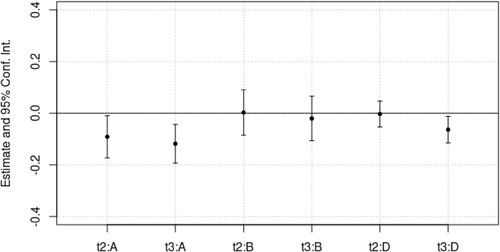
Ordinarily in DID analysis with multiple treatments and periods, there are various ways of testing the parallel trends assumption, including ‘placebo interactions.’ For example, Group B is not affected by the first downsizing, so parallel trends might imply that compared to Group C in t1, the coefficient on GroupB*t2 should not differ significantly from zero. Similarly, Group D is not affected by either downsizing, which might imply that compared to Group C in t1, the coefficients of GroupD*t2 or GroupD*t3 should not differ significantly from zero. Indeed, using Column (3) of Table 6 as the most credible, the coefficients on GroupB*t2, GroupD*t2, and GroupD*t3 are 0.003, -.003, and -.064, respectively, and only the last is significantly different from zero. A potential difficulty with some placebo interaction tests here, however, is that once downsizings begin, the baseline comparator Group C gains increased scarcity value from retaining access to CHS. This would provide a separate reason for its prices to rise relative to Group D in t2 and moreso in t3. Nonetheless, we illustrate these interaction coefficients and their 95% confidence intervals in Figure 9.

Figure 9. Treatment and parallel trend tests with 95% confidence intervals (Table 6 Column (3)).

Because of these confounds, our main parallel trends investigation will focus instead on the multiple years within period t1 before any downsizing, to test if the four groups moved in tandem.

Returning to Table 6 Columns (2) and (3), we add 18 interactions between each of Groups A, B and D with each of 2012 to 2017 year dummies. Group C in JanApril 2018 remains the omitted baseline.

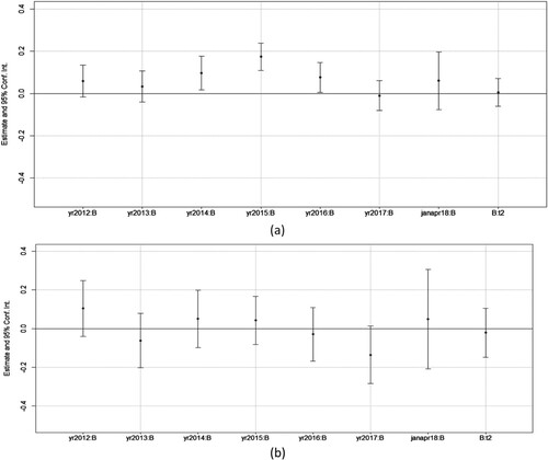
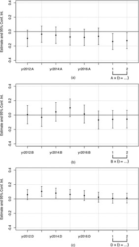
Beginning with pooled cross section (Column (4)), we note that with the 18 interaction terms added, the effect size of GroupA*t2 grows to −12.89% ($68,321), significant at 5%. The coefficient on GroupB*t3 remains negative, but compared to Column (2) is no longer significant. Moving to our parallel trend tests, we illustrate the 18 interaction terms in Figure 10, along with the t2 and t3 interaction terms. From Figure 10 (c) it is clear that in some pre-treatment years, the alternative non-treated Group D did not experience the same trends as non-treated Group C. More encouragingly, the difference in trends between treated Group A and (omitted) C tend to be reasonably small, in the range −4% to −10% from 2012 to 2017. The difference in trends between treated Group B and C are sometimes larger, within the range of 5% to −20%. However, none of the coefficients for Groups A vs. C or B vs. C are significantly different from zero. Thus a parallel trends assumption is not rejected in the pooled cross section between the two treated groups and the comparator untreated group, though the point estimates can appear far from zero for Group B for some years.

Figure 10. Coefficients for parallel trends tests based on Table 6 Column (4).

Moving to fixed effects in Column (5), we note first that our treatment outcomes differ slightly. The effect for GroupA*t2 reduces from −8.79% in Column (3) to −3.15% ($16,692), and loses statistical significance. We note the addition of the 18 interaction terms has substantially raised standard errors in Column (5), compared either to pooled cross section Column (4), or fixed effects without the interactions (Column (3)). The coefficient for Group B*t3 remains insignificant as in Column (3), again with a higher standard error than under pooled cross section. Moving to the parallel trends tests, Figure 11 shows that none of the 18 interaction coefficients are significant. Even tests comparing untreated Groups D and C are not significant, though the point estimates are far from zero. However, the confidence intervals are noticeably wider under fixed effects than pooled cross section. While insignificant, the point estimates of the gaps between Groups A and C during t1 range from 2% to 10%, and between Groups B and C between 2.5% and 11%.

Figure 11. Coefficients for parallel trends tests based on Table 6 Column (5).

Overall, based on these parallel trend results, we consider the DID estimations of potential treatment effects for Group A in t2 to be credible. Treatment effects range in Table 6 from non-significant −3.15% in Column (5), to −12.89% in Column (4). Tests indicate perhaps larger breaks from parallel trends between Groups B and C than between Groups A and C, but formally they remain insignificant, and thus treatment effect tests for B in t3 are also largely credible. Unlike the first downsizing, while the treatment effect point estimates from the second downsizing are uniformly negative, they are generally not significant, and never so under fixed effects (Columns (3) and (5)).

5.3 Robustness checks

We undertake numerous robustness checks of our main results. These include analysing the two downsizings separately, clustering standard errors to house, eliminating house sales after the second KPMG report was completed but not made public, eliminating house sales prior to 2015, and making Group D rather than C the omitted category. We also consider the effect of number of bedrooms on size of price effect, add quarterly or monthly dummies to control for seasonality, and vary how missing housing characteristics are addressed.

To study the first downsizing alone, we compare sales from Groups A and C in t1, compared to t2 and t3 combined. Similarly, to study the second downsizing alone, we compare only sales for Groups B and C, in t1 and t2 combined, compared to t3. The results are reported in Table 7 Panel A for the first downsizing, and Panel B for the second.

Table 7. Empirical results of analysing two downsizings separately.

Panel A:
	Column (1)	Column (2)	Column (3)	Column (4)	Column (5)
Dependent Variable:	LogHousePrices
GroupA*(t2 + t3)	−0.059**	−0.067****	−0.094***	−0.157***	−0.024
	(0.023)	(0.017)	(0.030)	(0.057)	(0.128)
N:	8090	8090	8090	8090	8090
R^2	0.106	0.542	0.274	0.534	0.274
Adjusted R^2	0.106	0.537	−2.019	0.528	−2.025
F-Statistics	319.545 on 3 and 8086 DF, p-value: < 2.22e-16	101.8 on 93 and 7996 DF, p-value: < 2.2e-16	91.713 on 8 and 1946 DF, p-value: < 2.22e-16	93.32 on 98 and 7991 DF, p-value: < 2.2e-16
	52.414 on 14 and 1940 DF, p-value: < 2.22e-16
Panel B:
	Column (1)	Column (2)	Column (3)	Column (4)	Column (5)
Dependent Variable:	LogHousePrices
GroupB*t3	−0.060*	−0.053**	−0.021	0.008	−0.021
	(0.035)	(0.026)	(0.048)	(0.033)	(0.065)
N:	7728	7728	7728	7728	7728
R^2	0.075	0.506	0.267	0.508	0.271
Adjusted R^2	0.075	0.500	−2.076	0.502	−2.070
F-Statistics	209.3 on 3 and 7724 DF, p-value: < 2.2e-16	83.05 on 94 and 7633 DF, p-value: < 2.2e-16	74.559 on 9 and 1841 DF, p-value: < 2.22e-16	78.03 on 101 and 7626 DF, p-value: < 2.2e-16	42.707 on 16 and 1834 DF, p-value: < 2.22e-16
Fixed effects:
Groups	Y	N	N	N	N
Periods	Y	N	N	N	N
HouseID	N	N	Y	N	Y
Year	N	Y	Y	Y	Y
House Features	N	Y	N	Y	N
Group T1 Year Interactions	N	N	N	Y	Y
Suburb	N	Y	N	Y	N

Notes: 1. Standard errors in parentheses.

2. Significance levels: ‘****’ 0.001 ‘***’ 0.01 ‘**’ 0.05 ‘*’ 0.1

Most of the first downsizing effect magnitudes and significance levels increase (Columns (1), (3) and (4)) when considered separately. Compared to Group C in t1, the Group A effect size now ranges from −2.37% but not significant (Column (5)) to −14.53% (Column (4)). In contrast, the second downsizing effects do not change much, with the most credible estimates remaining insignificant. We also conduct parallel trends tests for the two downsizings separately, with details in Appendix 5. For both downsizings, the parallel trends assumption is never rejected under fixed effects, but now rejected for a few year/group interactions under pooled cross section. As before, the test interaction terms under fixed effects have wide confidence intervals.

Next we cluster standard errors in our fixed effects Columns (3) and (5) in both Tables 6 and 7 to the level of House ID. We calculate cluster-robust variance estimators using CR1 estimation in the statistical package R, which multiplies the original form of the Sandwich estimator of Liang and Zeger (1986) by m/(m-1), where m is the number of clusters. Table 8 reports our findings.¹⁶ The results are virtually unchanged.

Table 8. Fixed effects with standard errors clustered to House ID.

Coefficients	Comparison results from	Original Result	Clustering SE on House ID
GroupA*t2	Table 6 Column (3)	−0.092**	−0.092***
		(0.042)	(0.035)
GroupB*t3		−0.021	−0.021
		(0.044)	(0.049)
GroupA*t2	Table 6 Column (5)	−0.032	−0.032
		(0.130)	(0.107)
GroupB*t3		−0.070	−0.705
		(0.120)	(0.113)
GroupA*(t2 + t3)	Table 7 Panel A Column (3)	−0.094***	−0.094****
		(0.030)	(0.019)
GroupA*(t2 + t3)	Table 7 Panel A Column (5)	−0.024	−0.024
		(0.128)	(0.079)
GroupB*t2	Table 7 Panel B Column (3)	−0.021	−0.021
		(0.048)	(0.041)
GroupB*t2	Table 7 Panel B Column (5)	−0.021	−0.022
		(0.065)	(0.052)

Notes: 1. Standard errors in parentheses.

2. Significance levels: ‘****’ 0.001 ‘***’ 0.01 ‘**’ 0.05 ‘*’ 0.1

To address any leakage of the un-released second KPMG report starting in October 2017, we next eliminate all house sales between October 1^st 2017 and April 4th 2018. Results are reported in Panel A of Appendix 7. With a new omitted time of Jan–Sept 2017, the GroupA*t2 interaction drops slightly in magnitude (from 8.75% to 7.63%) under fixed effects Column (3), and its significance level drops from 5% to 10%. Otherwise, results are similar. Not reported here, we instead eliminate all house sales from 2012 to 2014, to move further from the disruption of the earthquakes and make the three time periods of roughly equal length. While this reduces the number of house sales observations from N = 14738 to 8693, including crucial repeat sales for fixed effects, it strengthens the size and significance of the GroupA*t2 interaction terms in Columns (3), (4), and (5), for example to −15.28% in Column (3) is significant at the 1% rather than 10% level. Yet the second downsizing remains insignificant in Columns (3) - (5) as with the longer sample.

Next, given that some specifications of our main results (Columns (1) and (2)) find that Group D house prices were also falling relative to omitted Group C in periods t2 and t3, we test the stability of our results to making Group D rather than C our omitted baseline. Results are reported in Panel B of Appendix 7. Perhaps not surprisingly, in the models that originally showed Group D prices falling relative to C in t2 (Columns (1) and (2)), Group A price drops are no longer found significantly different to (also falling) omitted Group D prices. Whereas in the models that did not originally find D prices significantly falling relative to C in period t2 (Columns (3), (4) and (5)), Group A prices still lower significantly in the same cases as when C was omitted (Columns (3) and (4)).

We next asked if housing better suited to families with children in Groups A or B experienced greater house price effects from the downsizings. While we could have introduced interaction terms between number of bedrooms and period and group, calculation of overall treatment effects would become unwieldy. We opted instead for the simpler approach of eliminating housing with one or fewer bedrooms from the analysis to see if treatment effects increased. However because the area around CHS contains predominantly single family houses, this eliminated only 168 of 14,738 observations. Perhaps not surprisingly, this omission made no qualitative difference to the size or significance levels of our key treatment terms.

Next, recognizing that housing prices may be subject to seasonal effects we added either quarterly or monthly dummies. Either approach had no qualitative effect on the GroupA*t2 or GroupB*t3 interaction coefficients in Columns (1), (2), (3), or (5). Surprisingly, however, controlling for seasonality reduced the magnitude of the house price drop for Group A from −12.89% to −3.00% (monthly) or −3.72% (quarterly) in Column (4), the pooled cross section specification with Group/year interactions within t1. These lower magnitudes were no longer significant.

Lastly, for housing characteristics that had missing observations, rather than assigning them sample means or to a missing category, we try either omitting such houses from our pooled cross section models (2) and (4), or instead dropping the worst offending missing variable Number Garages. Not reported here, the first approach lowers our sample size from N = 14738 to N = 2015, and results in no interaction terms (treatment or placebo) being significant in Columns (2) or (4), though Group A point estimates remain negative. If we first drop Number Garages, our sample size recovers somewhat to N = 7418, and we find intermediate results, with GroupA*t2 similar to our main approach in Column (2) at −7.70% and significant at the 5% level, but losing significance with 18 interaction terms added in Column (4).

6. Discussion and conclusion

In this paper, we have used difference-in-differences (DID) to estimate the effect of two consecutive downsizings in access rights to a highly sought-after secondary school on housing sales prices in Christchurch, New Zealand. In our main analysis, we predominantly find a negative effect on housing prices from the first downsizing, with magnitude varying from a non-significant −3.15% in fixed effects with numerous interactions terms included, to a significant −12.89% in pooled cross section with the same interactions. In contrast, we find little evidence of a significant effect from the second downsizing, and never in fixed effects specifications, varying from a non-significant −2.08% to a significant −7.23%.

In greater detail, for the first downsizing, pooled cross section analysis that controls for measurable housing characteristics consistently finds negative effects. Fixed effects also finds the first downsizing lowers prices significantly by 8.75% if eighteen first period Year/Group interaction terms are excluded, but not if they are included. Fixed effects specifications better control for unobserved housing characteristics that may affect price, and pass parallel trends tests, but must identify price effects off a fewer number of repeat sales in key comparison groups.

We thus have mixed evidence that the first downsizing significantly lowered housing sales prices, and more consistent evidence that the second downsizing did not. These findings generally hold true across a wide range of robustness checks, whether we analyse the downsizings separately, cluster standard errors to house, omit early years or time close to when the first downsizing was announced publicly, change the omitted group from those always in-zone to those never in-zone, and so on.

Tests for parallel trends prior to the downsizings (using 18 year/group interaction terms) could not be rejected for fixed effects specifications, nor for most pooled cross section models, though with exceptions for some years if the downsizings were analysed separately. While parallel trends were not rejected for fixed effects models, such models tended to have larger standard errors/wider confidence intervals for both treatment and parallel trend tests than pooled cross section models, or even than fixed effects models without the additional interaction terms. As such, our fixed effects parallel trends tests cannot prove that parallel trends hold, only that they cannot be rejected.

We conclude that CHS’s first downsizing likely reduced housing sales prices in the affected area relative to remaining in zone, with the effect size (3.15%–8.75% in fixed effects) consistent with the existing literature, if somewhat modest given the dissimilarities of local alternative schools. The existing literature consistently finds school quality affects housing prices, though estimated effect size varies widely due to differences in institutions, data sources, and measurement methods. Focussing on a similar DID analysis, Bogart and Cromwell (2000) find that loss of access to a wealthy school district in Ohio is associated with a 9.9% housing price drop.

Our research has several limitations. First, we examine only one school’s downsizing, so caution must be applied in extrapolating the magnitude of effects found. Second, though our tests cannot reject parallel trends in the fixed effect nor most pooled cross section analysis, some relevant interaction term point estimates are still far from zero in some years prior to all downsizings. Third, for our pooled cross section models, there may be omitted house or amenity characteristics that affect sales prices which may affect both the direction and the size of our treatment effect estimates.

Nonetheless, this analysis provides the first difference-in-differences analysis of school zone effects on housing price in New Zealand. We hope our findings can help policymakers better understand spillover effects on housing affordability of using zone changes to promote equity of access to popular schools, and efficient utilization of existing networks.

Acknowledgement

We would like to acknowledge comments from two anonymous referees, attendants at the 2022 NZAE conference in Wellington, and in a seminar in the Department of Economics and Finance at the University of Canterbury. Special thanks is owed to Sussie Deng for her assistance with map drawing. This work was also made possible by the use of the Research Compute Cluster facilities at the University of Canterbury. Financial support for the purchase of CoreLogic housing sales data was provided by the Library of the University of Canterbury, while support for attendance at the NZAE conference was provided by Prof. Bob Reed and the Business School of the University of Canterbury.

Disclosure statement

No potential conflict of interest was reported by the authors.

Notes

1 For recent examples, see Black, 1999; Downes & Zabel, 2002; Brasington & Haurin, 2006; Clapp et al., 2008; and Chiodo, Hernández-Murillo, & Owyang, 2010.

2 Source: https://doi.org/10.1787/888932957498.

3 Alternative measures included value-added, peer racial and socio-economic composition, and pupil/teacher ratios.

4 https://www.educationcounts.govt.nz/statistics/.

5 The meshblock is a minimum aggregated census unit, consisting of roughly 50 households.

6 For detail on the decile system, see https://www.education.govt.nz/school/funding-and-financials/resourcing/operational-funding/school-decile-ratings/.

7 https://www.educationcounts.govt.nz/statistics/6028.

8 The 18 full year schools are Avonside Girls', Burnside, Cashmere, Catholic Cathedral, Christchurch Boys', Christchurch Girls', Hagley, Hillmorton, Hornby, Linwood, Mairehau, Marian, Papanui, Riccarton, Shirley Boys', St Bede’s, St Thomas of Canterbury, and Villa Maria. The 8 partial year schools are Hillview Christian, Emmanuel Christian, Middleton Grange, Haeata Community, Rudolf Steiner, and te reo Māori medium schools Te Pa o Rakaihautu, TKKM o Te Whanau Tahi, and TKKM o Waitaha.

9 Source: Education Counts (www.educationcounts.govt.nz).

10 See https://assets.education.govt.nz/public/Documents/Ministry/Information-releases/Responses-to-Official-Information-Act-Requests/KPMG-Christchurch-schools-report-1-of-2.pdf for the first report, and https://assets.education.govt.nz/public/Uploads/R-oia2-1099143.pdf for the second report.

11 See https://assets.education.govt.nz/public/Documents/1175116-Cashmere-High-School-Zoning.pdf.

12 See https://www.parliament.nz/en/pb/sc/reports/document/SCR_114554/petition-of-jo-bethell-review-of-proposed-rezone-of-cashmere?fbclid=IwAR0mDMzx5gZcark0UCN4AjWhSYyMPQj-0SRqUx7t4q4b6LIf6P3mM-vnsTA.

13 https://web.archive.org/web/20180217072710/http://www.cashmere.school.nz/enrolment/CHS-zone.html.

14 We have no evidence of differing degrees of earthquake damage between the neighbourhoods around CHS. However differences causes by slope of land should be picked up by controlling for Contour of property, or house fixed effects.

15 As the dependent variable is log-transformed, to get the percentage effect on housing price we exponentiate the coefficient, subtract one, and multiply by 100.

16 We use the coef-test() function from the clubSandwich package in R.

Appendix 1

Description of cashmere high school zones downsizings

Table

Original CHS Zone	First Downsizing	Second Downsizing
From the junction of Frankleigh Street and Sparks Road	Starting from the junction of Frankleigh Street / Sparks Road / Lyttleton Street,	Starting from the junction of Frankleigh Street / Sparks Road / Lyttelton Street;
Along Sparks Road to the intersection of Sparks and Rydal Street,	West along Sparks Road to the intersection of Sparks and Rydal Street,	West along Sparks Road to the intersection of Sparks and Rydal Street
Along Rydal, into Northaw into Rollesby Street,	South along Rydal Street to Northaw Street • West on Northaw Street to Rollesby Street (including addresses to 16 Northaw Street), • South on Rollesby Street to Rydal Street	South along Rydal Street to Northaw Street, West on Northaw Street to Rollesby Street (including addresses to 16 Northaw Street), South on Rollesby Street to Rydal Street
South along Rydal Street into Leistrella Road to the intersection with Hoon Hay Road.	South along Rydal Street to Leistrella Road	South along Rydal Street to Leistrella Road
South along Hoon Hay Road to Blakiston Street (including Barossa and Penmarc),	East on Leistrella Road to Hoon Hay Road (including all addresses on Leistrella Road up to number 35).	East on Leistrella Road to Hoon Hay Road (including all addresses on Leistrella Road up to number 35)
Along Kaiwara Street to Cashmere Road.	South along Hoon Hay Road to Blakiston Street (including Barossa Lane) • West on Blakiston Street to Kaiwara Street,	South along Hoon Hay Road to Blakiston Street (including Barossa Lane) West on Blakiston Street to Kaiwara Street
	North, then West and South on Kaiwara Street to Cashmere Road (including Penmarc Lane),	North, then West and South on Kaiwara Street to Cashmere Road (including Penmarc Lane)
West along Cashmere Road to Hoon Hay Valley Road,	West along Cashmere Road (including Boonwood Close) to Hoon Hay Valley Road,	West along Cashmere Road (including Boonwood Close) to Hoon Hay Valley Road
	Along Hoon Hay Valley Road to the southern end of the road, then	Along Hoon Hay Valley Road to the southern end of the road, then
Then across to the Summit Road and	Following a line directly across to the Summit Road / Worsleys Road intersection (including all Worsleys Road Addresses) and	Following a line directly across to the Summit Road / Worsleys Road intersection (including all Worsleys Road Addresses) and
Along the Summit Road to the junction with Gebbies Pass Road, including all residences with access from the Summit Road.	Along the Summit Road to the junction with Gebbies Pass Road (including all residences accessed from this portion of the Summit Road, including addresses 685, 703 and 706 Gebbies Pass Road),	Along the Summit Road to the junction with Gebbies Pass Road (including all residences accessed from this portion of the Summit Road, including addresses 685, 703 and 706 Gebbies Pass Road),
From the junction of Gebbies Pass and the Summit Roads to Port Levy, including all residences on the Port Levy Road and the Camp Bay Road and all other roads feeding to the south side of Lyttelton Harbour.	From the junction of Gebbies Pass and the Summit Road, in a straight line to Port Levy	From the junction of Gebbies Pass and the Summit Road, in a straight line to Port Levy
The remaining boundary shall run from the intersection of Frankleigh and Lyttelton Streets,
Northwards along the west of Lyttelton Street to Neville Street.	Including all residences on Purau Port levy Road, Camp Bay Road.	Including all residences on Purau Port Levy Road, Camp Bay Road.
East along Neville Street to Barrington Street.	Including addresses in Port Levy; including Old Port Levy Road, Wharf Road, Fields Road, Fernlea Point Road, addresses down to 1251 Western Valley Road, Richfield Road, addresses down to 899 Port Levy-Pigeon Bay Road, Pa Road, Jetty Road, Puari Road, and Putiki Road.	Including addresses in Port Levy; including Old Port Levy Road, Wharf Road, Fields Road, Fernlea Point Road, addresses down to 1251 Western Valley Road, Richfield Road, addresses down to 899 Port Levy-Pigeon Bay Road, Pa Road, Jetty Road, Puari Road, and Putiki Road.
Northwest along Barrington Street to Lincoln Road, then along Lincoln Road to Moorhouse Avenue.	From Port Levy, West along the coast line (past Diamond Harbour) to Governors Bay, then north east along the coast line to a point on the coast due west of 20 Park Terrace (in Corsair Bay),	From Port Levy, West along the coast line (past Diamond Harbour) to Governors Bay, then north east along the coast line to a point on the coast due west of 20 Park Terrace (in Corsair Bay)
East along Moorhouse Avenue to the junction of Waltham Road.	North along Park Terrace to Governors Bay Road,	North along Park Terrace to Governors Bay Road
South along Waltham Road to the intersection with Brougham Street	West along Governors Bay Road to 90 Governors Bay Road, then	West along Governors Bay Road to 90 Governors Bay Road, then
and then along Brougham Street to the intersection with Opawa Road	Following a line from 90 Governors Bay Road, north west to the Summit Road / Rapaki Road (Track) intersection.	Following a line from 90 Governors Bay Road, north west to the Summit Road / Rapaki Road (Track) intersection
In a south easterly direction along Opawa Road to its junction with Port Hills Road.	North along Rapaki Road to 90 Rapaki Road, then	North along Rapaki Road to 90 Rapaki Road, then
West covering streets along the south side of the Port Hills Road to Rapaki Road.	Following a line north to the Port Hills Road / Opawa Road (SH76) intersection (including addresses 361-385 Port Hills Road)	Following a line north to the Port Hills Road / Opawa Road (SH76) intersection (including addresses 361-385 Port Hills Road)
South along Rapaki Road to its junction with Summit Road.		West along Port Hills Road to Centaurus Road (including Lucienne Place)
From the junction of Rapaki Road and the Summit Road in a straight line to the eastern end of Corsair Bay, to include the house at number 20 Park Terrace.	North on Opawa Road (SH76) to Opawa Road,	West along Centaurus Road to Aynsley Terrace
		North along Aynsley Terrace to address number 75-75A
		West to the $\overline{\mathrm{O}}$p$\overline{\mathrm{a}}$waho / Heathcote River
		West along the South bank of the $\overline{\mathrm{O}}$p$\overline{\mathrm{a}}$waho / Heathcote River to the Wilsons Road Bridge
		North west to the Wilsons Road / Waltham Road / Eastern Terrace intersection
		South west along Eastern Terrace to Tennyson Street
		West along Tennyson Street to Southampton Street
		North along Southampton Street to Croydon Street (including Ikamatua Lane)
		North east along Croydon Street to Huxley Street
		North west along Huxley Street to Colombo Street
	West on Opawa Road, across the river to Brougham Street,	North along Colombo Street to Brougham Street (SH76)
	West on Brougham Street to Selwyn Street,	West on Brougham Street (SH76) to Selwyn Street
	South along Selwyn Street to Coronation Street,	South along Selwyn Street to Coronation Street
	South west along Coronation Street to Barrington Street,	South west along Coronation Street to Barrington Street
	South along Barrington Street to Stourbridge Street (including Sefton Place and Kinver Place)	South along Barrington Street to Stourbridge Street (including Sefton Place and Kinver Place)
	South west along Stourbridge Street to Lyttelton Street	South west along Stourbridge Street to Lyttelton Street
	South along Lyttelton Street to the junction with Frankleigh Street and Sparks Road.	South along Lyttelton Street to the junction with Frankleigh Street and Sparks Road.

Appendix 2: illustration of canonical two-way fixed effect DID model

Table

Y	Control Group	Treatment Group	Across-group Difference	Difference-in-Differences
Pre-treatment Period(T = 0)	E{Yit|D = 0, T = 0}	E{Yit|D = 1, T = 0}	E{Yit|D = 1, T = 0}- E{Yit|D = 0, T = 0}	Across-group Difference of Post-Treatment Period minus Across-group Difference from the Pre-Treatment Period: (E{Yit|D = 1, T = 1}- E{Yit|D = 0, T = 1})- (E{Yit|D = 1, T = 0}- E{Yit|D = 0, T = 0})
Post-Treatment Period(T = 1)	E{Yit|D = 0, T = 1}	E{Yit|D = 1, T = 1}	E{Yit|D = 1, T = 1}- E{Yit|D = 0, T = 1}
Across-time Difference	E{Yit|D = 0, T = 1} - E{Yit|D = 0, T = 0}	E{Yit|D = 1, T = 1} - E{Yit|D = 1, T = 0}
Difference-in-Differences				${\tau }_{\mathrm{ATE}}$ = E{Yit|D = 1, T = 1}+ E{Yit|D = 0, T = 0}- E{Yit|D = 1, T = 0}- E{Yit|D = 0, T = 1})-
	Across-time Difference of Treatment Group minus Across-time Difference of Control Group: (E{Yit|D = 1, T = 1} - E{Yit|D = 1, T = 0})- (E{Yit|D = 0, T = 1} - E{Yit|D = 0, T = 0})

Appendix 3: explanation of expanded two-treatment four-Group three-period DID model

(8) $\begin{array}{rl}{Y}_{\mathrm{it}}& ={\alpha }_i+{\beta }_1\mathrm{GroupA}+{\beta }_2\mathrm{GroupB}+{\beta }_3\mathrm{GroupD}+{\gamma }_{1}t2+{\gamma }_{2}t3+\sum _1^i{\theta }_i{X}_i+\sum _1^t{\eta }_t\mathrm{Yea}{r}_t+{\rho }_1\mathrm{GroupA}\ast t2\\ & +{\rho }_2\mathrm{GroupA}\ast t3+{\rho }_3\mathrm{GroupB}\ast t2+{\rho }_4\mathrm{GroupB}\ast t3+{\rho }_5\mathrm{GroupD}\ast t2+{\rho }_6\mathrm{GroupD}\ast t3+{\epsilon }_{\mathrm{it}}\end{array}$(8)

Table 5.3. Interpretation of coefficient meanings in model (8)

Table

Terms	Coefficient	Calculation of differences	Interpretation
$\mathrm{GroupA}\ast t2$	${\rho }_1$	$=(\overline{y_{A,t2}}-\overline{y_{A,t1}})-(\overline{y_{C,t2}}-\overline{y_{C,t1}})$	delta Y2- delta Y1 across group A and C, or delta YA- delta YC across Periods t2 t1
$\mathrm{GroupA}\ast t3$	${\rho }_2$	$=(\overline{y_{A,t3}}-\overline{y_{A,t1}})-(\overline{y_{C,t3}}-\overline{y_{C,t1}})$	delta Y3- delta Y1 across group A and C, or delta YA- delta YC across Periods t3 t1
$\mathrm{GroupB}\ast t2$	${\rho }_3$	$=(\overline{y_{B,t2}}-\overline{y_{B,t1}})-(\overline{y_{C,t2}}-\overline{y_{C,t1}})$	delta Y2- delta Y1across group B and C, or delta YB- delta YC across Periods t2 t1
$\mathrm{GroupB}\ast t3$	${\rho }_4$	$=(\overline{y_{B,t3}}-\overline{y_{B,t1}})-(\overline{y_{C,t3}}-\overline{y_{C,t1}})$	delta Y3- delta Y1 across group B and C, or delta YB- delta YC across Periods t3 t1
$\mathrm{GroupD}\ast t2$	${\rho }_5$	$=(\overline{y_{D,t2}}-\overline{y_{D,t1}})-(\overline{y_{C,t2}}-\overline{y_{C,t1}})$	delta Y2- delta Y1 across group D and C, or delta YD- delta YC across Periods t2 t1
$\mathrm{GroupD}\ast t3$	${\rho }_6$	$=(\overline{y_{D,t3}}-\overline{y_{D,t1}})-(\overline{y_{C,t3}}-\overline{y_{C,t1}})$	delta Y3- delta Y1 across group D and C, or delta YD- delta YC across Periods t t31
Constant	${\alpha }_i$		Group mean of C in t1
group A	${\beta }_1$		Group difference between A and C in t1
group B	${\beta }_2$		Group difference between B and C in t1
group D	${\beta }_3$		Group difference between D and C in t1
t2	${\gamma }_1$		Period difference between t2 and t1 of C
t3	${\gamma }_2$		Period difference between t3 and t1 of C

Appendix 4: fixed effect parallel trend test regression (Corresponding to column (5) in table 6)

Table

Dependent Variable:	LogHousePrices
GroupA*t2	−0.086
	(0.054)
GroupB*t2	−0.104
	(0.067)
GroupD*t2	0.0077
	(0.037)
GroupA*t3	−0.115**
	(0.054)
GroupB*t3	−0.125*
	(0.067)
GroupD*t3	−0.057
	(0.038)
t2	0.357****
	(0.026)
t3	0.531****
	(0.026)
Year2013*A	0.008
	(0.061)
Year2014*A	0.043
	(0.063)
Year2015*A	−0.007
	(0.056)
Year2016*A	0.011
	(0.061)
Year2017*A	−0.037
	(0.063)
Year2018JanApr*A	−0.054
	(0.129)
Year2013*B	−0.166
	(0.076)
Year2014*B	−0.054
	(0.079)
Year2015*B	−0.062**
	(0.066)
Year2016*B	−0.134*
	(0.075)
Year2017*B	−0.239***
	(0.079)
Year2018JanApr*B	−0.055
	(0.126)
Year2013*D	0.018
	(0.043)
Year2014*D	0.045
	(0.041)
Year2015*D	−0.020
	(0.040)
Year2016*D	0.043
	(0.042)
Year2017*D	0.037
	(0.044)
Year2018JanApr*D	−0.061
	(0.069)
Fixed effects:
Groups	N
Periods	N
Houseid	Y
Year	Y
N:	14738
R^2	0.282
Adjusted R^2	−1.93
F-statistics	44.274 on 32 and 3613 DF, p-value: < 2.22e-16

Notes: 1. Standard errors are reported in parentheses.

2. Significance codes: ‘****’ 0.001 ‘***’ 0.01 ‘**’ 0.05 ‘*’ 0.1.

Appendix 5. Details of parallel trends tests for two downsizings analysed separately

Regarding the parallel trends test for the first downsizing alone, we focus on adding interactions between Group A and t1 year dummies in Columns (4) and (5) of Table 7’s Panel A, and between Group B and t1 year dummies in Columns (4) and (5) of Table 7’s Panel B. The first downsizing’s added interaction terms are illustrated in Appendix Figure 5.1 (a) for the Column (4) model, and Appendix Figure 5.1 (b) for the Column (5) model.

Figure 5.1 (a) indicates that, compared to Group C in JanApril 2018, the price changes in Groups C and A are not in parallel in either 2012 or 2016 in pooled cross section. In contrast, with wider confidence intervals under fixed effects as shown in Figure 5.1 (b), none of the interactions differ significantly from zero. Thus, taken at face value, for the first downsizing parallel trends appear better supported for the fixed effects specifications than for the pooled cross section, though this could be caused by fixed effects having more imprecise estimates caused by relying on fewer repeat sales in key comparison groups.

Regarding the parallel trends test for the second downsizing alone (B vs. C), these are illustrated in Appendix Figure 5.2 (a) and (b). Again for the pooled cross section in Figure 5.2 (a) parallel trends are rejected for the years 2014, 2015 and 2016, but with wider confidence intervals under fixed effects they are never rejected in Figure 5.2 (b). We discuss the implications of these findings in the Conclusion.

Figure 5.1 Coefficients for Parallel Trends Tests for Table 7 Panel A, Columns (4) and (5)

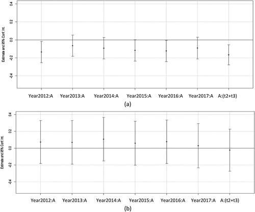
Figure 5.2 Coefficients for Parallel Trends Tests for Table 7 Panel B, Columns (4) and (5)

Appendix 6: eliminating sales after KPMG report, and making group D omitted baseline

Table

Drop Sales Oct 1^st 2017 – Apr 4th 2018
	Column (1)	Column (2)	Column (3)	Column (4)	Column (5)
Dependent Variable:	Log House Prices
GroupA*t2	−0.048*	−0.072****	−0.079**	−0.082**	−0.027
	(0.028)	(0.021)	(0.041)	(0.035)	(0.071)
GroupB*t2	−0.035	−0.084****	0.005	−0.001	−0.130*
	0.032	(0.024)	(0.045)	(0.036)	(0.074)
GroupD*t2	−0.045**	−0.059****	−0.003	−0.032	0.018
	(0.018)	(0.014)	(0.026)	(0.022)	(0.045)
GroupA*t3	−0.077***	−0.060***	−0.122***	−0.070**	−0.069
	(0.029)	(0.022)	(0.039)	(0.035)	(0.069)
GroupB*t3	−0.072**	−0.080***	−0.023	0.003	0.103
	(0.033)	(0.025)	(0.044)	(0.036)	(0.075)
GroupD*t3	−0.067****	−0.055****	−0.070***	−0.028	−0.049
	(0.020)	(0.015)	(0.027)	(0.023)	(0.045)
N:	14016	14016	14016	14016	14016
R^2	0.152	0.530	0.286	0.532	0.289
Adjusted R^2	0.152	0.527	−2.01	0.527	−2.01
Groups	Y	N	N	N	N
Periods	Y	N	N	N	N
House ID	N	N	Y	N	Y
Years	N	Y	Y	Y	Y
House Features	N	Y	N	Y	N
Suburbs	N	Y	N	Y	N
Group T1 Year Interactions	N	N	N	Y	Y
Imputed Missing Values	N	Y	N	Y	N
Omitting Group D Rather Than Group CColumn (1) Column (2) Column (3) Column (4) Column (5)
Dependent Variable:	Log House Prices
GroupA*t2	−0.009	−0.019	−0.088**	−0.145**	−0.100
GroupB*t2	(0.029)	(0.022)	(0.042)	(0.058)	(0.131)
GroupC*t2	0.007	−0.024	0.006	−0.067	−0.118
GroupA*t3 GroupB*t3	0.032	(0.024)	(0.045)	(0.064)	(0.120)
GroupC*t3	0.039**	0.054****	0.003	−0.007	−0.069
	(0.018)	(0.014)	(0.026)	(0.034)	(0.067)
	−0.016	−0.011	−0.054	−0.137**	−0.065
	(0.030)	(0.022)	(0.039)	(0.058)	(0.128)
	−0.008	−0.025	0.043	−0.069	−0.075
	(0.033)	(0.025)	(0.044)	(0.064)	(0.120)
	0.061***	0.049****	0.064**	−0.012	−0.005
	(0.019)	(0.015)	(0.026)	(0.034)	(0.067)
N:	14738	14738	14738	14738	14738
R^2	0.148	0.529	0.277	0.531	0.282
Adjusted R^2	0.148	0.526	−1.933	0.527	−1.93
Groups	Y	N	N	N	N
Periods	Y	N	N	N	N
House ID	N	N	Y	N	Y
Years	N	Y	Y	Y	Y
House Features	N	Y	N	Y	N
Suburbs	N	Y	N	Y	N
Group T1 Year Interactions	N	N	N	Y	Y
Imputed Missing Values	N	Y	N	Y	N

Notes: 1. Standard errors in parentheses.

2. Significance levels: ‘****’ 0.001 ‘***’ 0.01 ‘**’ 0.05 ‘*’ 0.1

References

- Atkinson, S. E., & Crocker, T. D. (1987). A Bayesian approach to assessing the robustness of hedonic property value studies. Journal of Applied Econometrics, 2(1), 27–45. doi:10.1002/jae.3950020103
- Bae, H., & Chung, I. H. (2013). Impact of school quality on house prices and estimation of parental demand for good schools in Korea. KEDI Journal of Educational Policy, 10(1), 43–61.
- Barrow, L. (2002). School choice through relocation: Evidence from the Washington, DC area. Journal of Public Economics, 86(2), 155–189. doi:10.1016/S0047-2727(01)00141-4
- Bayer, P., Ferreira, F., & McMillan, R. (2007). A unified framework for measuring preferences for schools and neighborhoods. Journal of Political Economy, 115(4), 588–638. doi:10.3386/w13236
- Belfield, C. R. (2004). Modeling school choice: A comparison of public, private-independent, private-religious and home-schooled students. Education Policy Analysis Archives, 12, 30–30. doi:10.14507/epaa.v12n30.2004
- Bifulco, R., Ladd, H. F., & Ross, S. L. (2009). Public school choice and integration evidence from durham, North Carolina. Social Science Research, 38(1), 71–85. doi:10.1016/j.ssresearch.2008.10.001
- Black, S. E. (1999). Do better schools matter? Parental valuation of elementary education. The Quarterly Journal of Economics, 114(2), 577–599. doi:10.1162/003355399556070
- Black, S. E., & Machin, S. (2011). Chapter 10 Housing valuations of school performance. In E. A. Hanushek, S. Machin, & L. Woessman (Eds.), Handbook of the economics of education (Vol. 3, pp. 485–519). Elsevier. doi:10.1016/B978-0-444-53429-3.00010-7
- Bogart, W. T., & Cromwell, B. A. (2000). How much is a neighborhood school worth? Journal of Urban Economics, 47(2), 280–305. doi:10.1006/juec.1999.2142
- Bond, S. (2007). Cell phone tower proximity impacts on house prices: A New Zealand case study. Pacific Rim Property Research Journal, 13(1), 63–91. doi:10.1080/14445921.2007.11104223
- Brasington, D. (1999). Which measures of school quality does the housing market value? Journal of Real Estate Research, 18(3), 395–413. doi:10.1080/10835547.1999.12091004
- Brasington, D., & Haurin, D. R. (2006). Educational outcomes and house values: A test of the value added approach. Journal of Regional Science, 46(2), 245–268. doi:10.1111/j.0022-4146.2006.00440.x
- Brehm, M., Imberman, S. A., & Naretta, M. (2017). Capitalization of charter schools into residential property values. Education Finance and Policy, 12(1), 1–27. doi:10.1162/EDFP_a_00192
- Card, D., & Krueger, A. B. (1992). Does school quality matter? Returns to education and the characteristics of public schools in the United States. Journal of Political Economy, 100(1), 1–40. doi:10.1086/261805
- Chiodo, A., Hernández-Murillo, R., & Owyang, M. T. (2010). Nonlinear effects of school quality on house prices. Federal Reserve Bank of St. Louis Review, 92, 185–204. doi:10.20955/R.92
- Cho, M. (1996). House price dynamics: A survey of theoretical and empirical issues. Journal of Housing Research, 7(2), 145–172. http://www.jstor.org/stable/24832857
- Clapp, J. M., Nanda, A., & Ross, S. L. (2008). Which school attributes matter? The influence of school district performance and demographic composition on property values. Journal of Urban Economics, 63(2), 451–466. doi:10.1016/j.jue.2007.03.004
- Crone, T. M. (2006). Capitalization of the quality of local public schools: What do home buyers value? (Federal Reserve Bank of Philadelphia Working Paper No. 06-15). doi:10.2139/ssrn.928452
- Davidoff, I., & Leigh, A. (2008). How much do public schools really cost? Estimating the relationship between house prices and school quality. Economic Record, 84(265), 193–206. doi:10.1111/j.1475-4932.2008.00462.x
- Dougherty, J., Harrelson, J., Maloney, L., Murphy, D., Smith, R., Snow, M., & Zannoni, D. (2009). School choice in suburbia: Test scores, race, and housing markets. American Journal of Education, 115(4), 523–548. doi:10.1086/599780
- Downes, T. A., & Zabel, J. E. (2002). The impact of school characteristics on house prices: Chicago 1987–1991. Journal of Urban Economics, 52(1), 1–25. doi:10.1016/S0094-1190(02)00010-4
- Edmunds, S. (2017, August). Data shows NZ school zoning makes huge difference to house prices. Stuff. https://www.stuff.co.nz/business/95390822/data-shows-school-zones-make-significant-difference-to-house-prices.
- Education and Training Act (2020). https://www.legislation.govt.nz/act/public/2020/0038/latest/whole.html#LMS170676.
- Fack, G., & Grenet, J. (2010). When do better schools raise housing prices? Evidence from Paris public and private schools. Journal of Public Economics, 94(1-2), 59–77. doi:10.1016/j.jpubeco.2009.10.009
- Fernandez, M. A. (2019). A review of applications of hedonic pricing models in the New Zealand housing market. Auckland: Auckland Council.
- Figlio, D. N., & Lucas, M. E. (2004). What's in a grade? School report cards and the housing market. American Economic Review, 94(3), 591–604. doi:10.1257/0002828041464489
- Figlio, D. N., & Page, M. E. (2003). Can school choice and school accountability successfully coexist?. In C. M. Hoxby (Ed.), The economics of school choice (pp. 49–66). Chicago, IL: University of Chicago Press. doi:10.7208/chicago/9780226355344.003.0003.
- Fleming, D., Grimes, A., Lebreton, L., Maré, D., & Nunns, P. (2018). Valuing sunshine. Regional Science and Urban Economics, 68, 268–276. doi:10.1016/j.regsciurbeco.2017.11.008
- Gibbons, S., & Machin, S. (2006). Paying for primary schools: Admission constraints, school popularity or congestion? The Economic Journal, 116(510), C77–C92. doi:10.1111/j.1468-0297.2006.01077.x
- Gibbons, S., Machin, S., & Silva, O. (2013). Valuing school quality using boundary discontinuities. Journal of Urban Economics, 75, 15–28. doi:10.1016/j.jue.2012.11.001
- Gibson, J., & Boe-Gibson, G. (2014). Capitalizing Performance of ‘Free’ Schools and the Difficulty of Reforming School Attendance Boundaries. Department of Economics Working Paper 8/14, University of Waikato.
- Gibson, J., Sabel, C., Boe-Gibson, G., & Kim, B. (2005). House prices and school zones: Doesgeography matter? Paper presented at the New Zealand association of economists conference, June 2005.
- Goodman, A. C., & Thibodeau, T. G. (2003). Housing market segmentation and hedonic prediction accuracy. Journal of Housing Economics, 12(3), 181–201. doi:10.1016/S1051-1377(03)00031-7
- Haisken-DeNew, J., Hasan, S., Jha, N., & Sinning, M. (2018). Unawareness and selective disclosure: The effect of school quality information on property prices. Journal of Economic Behavior & Organization, 145, 449–464. doi:10.1016/j.jebo.2017.11.015
- Han, X., Shen, Y., & Zhao, B. (2021). Winning at the starting line: The primary school premium and housing prices in Beijing. China Economic Quarterly International, 1(1), 29–42. doi:10.1016/j.ceqi.2020.12.001
- Huang, B., He, X., Xu, L., & Zhu, Y. (2020). Elite school designation and housing prices-quasi-experimental evidence from Beijing, China. Journal of Housing Economics, 50, 1–18. doi:10.1016/j.jhe.2020.101730
- Hyman, D. N., & Pasour JrE. C. (1973). Reducing property Taxes in North Carolina: An Economic Analysis (No. 1908-2017-1923). https://doi.org/10.22004/ag.econ.259537.
- Jud, G. D., & Watts, J. M. (1981). Schools and housing values. Land Economics, 57(3), 459–470. doi:10.2307/3145886
- Lancaster, K. J. (1966). A new approach to consumer theory. Journal of Political Economy, 74(2), 132–157. doi:10.1086/259131
- Leech, D., & Campos, E. (2003). Is comprehensive education really free?: A case-study of the effects of secondary school admissions policies on house prices in one local area. Journal of the Royal Statistical Society: Series A (Statistics in Society), 166(1), 135–154. doi:10.1111/1467-985x.00263
- Li, M. M., & Brown, H. J. (1980). Micro-neighborhood externalities and hedonic housing prices. Land Economics, 56(2), 125–141. doi:10.2307/3145857
- Liang, K. Y., & Zeger, S. L. (1986). Longitudinal data analysis using generalized linear models. Biometrika, 73, 13–22. doi:10.1093/biomet/73.1.13
- Machin, S., & Salvanes, K. G. (2007, April). School choice and the housing market: Valuation through an admission policy reform. Royal economic society’s annual conference.
- Maguire, M. (2019). Equality and justice in education policy. Journal of Education Policy, 34(3), 299–301. doi:10.1080/02680939.2019.1591709
- Malpezzi, S. (2003). Hedonic pricing models: A selective and applied review. Housing Economics and Public Policy, 1, 67–89. doi:10.1002/9780470690680.ch5
- McClay, S., & Harrison, R. (2003). The impact of schooling zoning on residential house prices in Christchurch. Paper presented at the New Zealand association of economists conference, June 2003.
- Ministry of Education. (2019). Ngā Kura o Aotearoa: New Zealand Schools (2019). https://www.educationcounts.govt.nz/publications/schooling/2523/nga-kura-o-aotearoa-new-zealand-schools-2019.
- Ministry of Education. (2021). Ngā Kura o Aotearoa: New Zealand Schools (2020). https://www.educationcounts.govt.nz/publications/schooling/2523/nga-kura-o-aotearoanew-zealand-schools-2020
- New Zealand Education Review Office. (2019). Report for cashmere high school-06/06/2019. https://ero.govt.nz/institution/340/cashmere-high-school
- Nguyen-Hoang, P., & Yinger, J. (2011). The capitalization of school quality into house values: A review. Journal of Housing Economics, 20(1), 30–48. doi:10.1016/j.jhe.2011.02.001
- Oates, W. E. (1969). The effects of property taxes and local public spending on property values: An empirical study of tax capitalization and the tiebout hypothesis. Journal of Political Economy, 77(6), 957–971. doi:10.1086/259584
- OECD. (2019). Balancing school choice and equity an international perspective based on pisa. https://www.oecd-ilibrary.org/education/freedom-for-parents-to-choose-a-public-school-for-their-children-2009_c99de9e4-en
- OECD. (2021). Education at a Glance 2021. https://doi.org/10.1787/b35a14e5-en
- Plimmer, C. (2014). A time varying study of water view premiums in relation to residential house prices (Doctoral dissertation), Lincoln University.
- Rehm, M., & Filippova, O. (2008). The impact of geographically defined school zones on house prices in New Zealand. International Journal of Housing Markets and Analysis, 1(4), 313–336. doi:10.1108/17538270810908623
- Ries, J., & Somerville, T. (2010). School quality and residential property values: Evidence from Vancouver rezoning. The Review of Economics and Statistics, 92(4), 928–944. doi:10.1162/rest_a_00038
- Rosen, H. S., & Fullerton, D. J. (1977). A note on local tax rates, public benefit levels, and property values. Journal of Political Economy, 85(2), 433–440. doi:10.1086/260575
- Rosen, S. (1974). Hedonic prices and implicit markets: Product differentiation in pure competition. Journal of Political Economy, 82(1), 34–55. doi:10.1086/260169
- Schleicher, A. (2019). PISA 2018: Insights and interpretations. OECD. https://www.oecd.org/pisa/PISA%202018%20Insights%20and%20Interpretations%20FINAL%20PDF.pdf
- Seo, Y., & Simons, R. (2009). The effect of school quality on residential sales price. Journal of Real Estate Research, 31(3), 307–328. doi:10.1080/10835547.2009.12091255
- Tiebout, C. M. (1956). A pure theory of local expenditures. Journal of Political Economy, 64(5), 416–424. doi:10.1086/257839
- Turnbull, G. K., & Zheng, M. (2021). A meta-analysis of school quality capitalization in US house prices. Real Estate Economics, 49(4), 1120–1171. doi:10.1111/1540-6229.12300
- Walden, M. (1990). Magnet schools and the differential impact of school quality on residential property values. Journal of Real Estate Research, 5(2), 221–230. doi:10.1080/10835547.1990.12090619
- Wang, X., Yuan, Z., Min, S., & Rozelle, S. (2021). School quality and peer effects: Explaining differences in academic performance between China’s migrant and rural students. The Journal of Development Studies, 57(5), 842–858. doi:10.1080/00220388.2020.1769074
- Wen, H., Xiao, Y., & Zhang, L. (2017). School district, education quality, and housing price: Evidence from a natural experiment in Hangzhou, China. Cities, 66, 72–80. doi:10.1016/j.cities.2017.03.008
- Wilkes, M. (2020, July). Paying a premium for a house in a school zone is a risk rather than an investment. Stuff. https://www.stuff.co.nz/life-style/homed/buying/122113840/paying-a-premium-for-a-house-in-a-school-zone-is-a-risk-rather-than-an-investment.
- Yadavalli, A. P., & Florax, R. J. (2013). The effect of school quality on house prices: A meta-regression analysis. Paper presented at 2013 Agricultural and Applied Economics Association Annual Meeting, Washington, DC. https://ageconsearch.umn.edu/record/151291
- Zhang, J., Li, H., Lin, J., Zheng, W., Li, H., & Chen, Z. (2020). Meta-analysis of the relationship between high quality basic education resources and housing prices. Land Use Policy, 99, 1–9. doi:10.1016/j.landusepol.2020.104843