Monetary policy independence in an era of financial globalization: what theory suggests and the data in Oceania say

ABSTRACT

This paper shows that under a floating exchange rate and integrated financial markets an optimizing central bank concerned about price and output stability partly accommodates a change in monetary policy abroad. A positive co-movement between the domestic policy rate and the foreign interest rate does not indicate lack of monetary policy independence but is an outcome of optimal policymaking in an open economy deeply embedded in the global financial architecture. Empirical evidence on overnight interest rate changes in Oceania (New Zealand, Australia) and US federal funds rate changes is consistent with this view.

JEL:

• Codes: E3
• E5
• F3

KEYWORDS:

• Policy independence
• optimal policy response
• correlation of interest rates
• high capital mobility

1. Introduction

The argument that the existence of a global financial cycle prevents countries that maintain a flexible exchange regime from conducting an independent monetary policy, first raised by Rey (2016) in her Mundell-Fleming lecture, has received considerable attention in the recent literature. Her claim that the Mundellian Trilemma has morphed into a dilemma has drawn support from Jeanne (2022) but also encountered skeptical comments from Obstfeld (2021) and fierce criticism by Nelson (2020). The evidence for Rey’s argument rests heavily on the empirical observation that interest rates in small and medium-sized economies are positively correlated with the policy stance in the United States, the country that sets the pace for the global financial cycle.

This paper shows that under a floating exchange rate and integrated financial markets an optimizing central bank, acting under discretion to achieve domestic objectives, generates a positive co-movement between the domestic and the foreign interest rate in a small open economy model. If monetary policy abroad changes, the policy rate in the small open economy adjusts in the same direction. This result holds irrespective of the degree of openness on both the demand and supply side, the relative aversion of the central bank to inflation variability, and violation of the uncovered interest rate parity condition. A positive co-movement between the domestic and foreign interest rate does not indicate lack of monetary policy independence but is an outcome of optimal policymaking in an open economy deeply embedded in the global financial architecture. In view of the high degree of capital mobility, the response of the real exchange rate is conditioned on the optimal interest rate reaction.

In the next section we lay out an open economy model. Section 3 elaborates on optimal policy and shows that the optimal inflation-output tradeoff depends on parameters that appear on both the supply and the demand side of the aggregate economy. The key contribution of the paper, the positive correlation between the domestic and foreign interest rate, is established in Section 4. The hypothesized co-movement of interest rates in the model is tested on data from Oceania and the United States in Section 5. The same section also examines the correlation between real exchange rates in Oceania and interest rate changes in the United States. A brief conclusion appears in Section 6.

2. The model

The framework consists of a micro-founded stochastic model of a small open economy similar to the one proposed by Guender (2006). The components include an open economy Phillips curve, an aggregate demand relation, a relation between the interest rates and the exchange rate under high capital mobility, and a relation between the CPI inflation rate, the domestic inflation rate, and the exchange rate under perfect exchange rate pass-through. (1) $\begin{array}{rl}& {\pi }_t=\beta E_t{\pi }_{t+1}+\kappa y_t+b{q}_t+u_t\end{array}$(1) (2) $\begin{array}{rl}& y=E_t{y}_{t+1}-a_1(i_t-E_t{\pi }_{t+1}^{\mathrm{CPI}})+a_2(q_t-E_t{q}_{t+1})+a_3(y_t^f-E_t{y}_{t+1}^f)+v_t\end{array}$(2) (3) $\begin{array}{rl}& i_t-E_t{\pi }_{t+1}-(i_t^f-E_t{\pi }_{t+1}^f)=-\varphi (E_t{q}_{t+1}-q_t)+{\epsilon }_t\end{array}$(3) (4) $\begin{array}{rl}& {\pi }_t^{\mathrm{CPI}}={\pi }_t+\gamma \mathrm{\Delta }{q}_t\end{array}$(4) where $a_1=(1-\gamma )\sigma a_2=\gamma (1-\gamma )\eta +{\eta }^f{\gamma }^f.$All parameters except $\varphi$are positive. $\gamma$ = the weight on the price of the foreign good in the definition of the CPI, $\sigma$ =  the intertemporal elasticity of substitution of consumption, and $\eta$ =  the elasticity of substitution between domestic and foreign consumption in the home country. The superscript f denotes foreign.

${\pi }_t=$ the rate of domestic inflation,$E_t{\pi }_{t+1}^{\mathrm{CPI}}=$ the expected rate of CPI inflation, $q_t=$ the real exchange rate^, $y_t$ =  the output gap, $i_t=$ the nominal rate of interest (the policy instrument), $i_t^f=$ the foreign nominal rate of interest, $E_t{\pi }_{t+1}^f=$ the expected foreign rate of inflation, $y_t^f$ = the foreign output gap. All foreign variables and additive shocks are treated as exogenous random variables with known distributions.¹

If $\varphi =-1$ in Equation (3) uncovered interest rate parity (UIP) holds. $\gamma$ represents the degree of openness on the demand side. On the supply-side the degree of openness is represented by the parameter b, which captures the importance of a real exchange rate channel in the Phillips curve.²

The central bank’s objective is to minimize variability in the output gap and domestic inflation.³ (5) $\sum _{j=0}^{\mathrm{\infty }}{\beta }^j(y_{t+j}^2+\mu {\pi }_{t+j}^2)0<\beta \le 1$(5)

3. Optimal discretionary policy

The central bank minimizes the objective function subject to the constraints of the model, given by Equations (1)–(4).⁴ The optimizing condition, referred to as the target rule, relates the two target variables to each other. This condition describes the trade-off between inflation and the output gap: (6) $\begin{array}{rl}{\pi }_t& =-\theta y_t\end{array}$(6) $\begin{array}{rl}\theta & =\frac{1}{\mu \left[\kappa +\frac{b}{\gamma ((1-\gamma )\eta +{\eta }^f{\gamma }^f)+(1-\gamma )\sigma (-\varphi -\gamma )}\right]}\end{array}$Here we observe that the degree of openness on the demand side ($(\gamma )$, the degree openness on the supply side (b), the parameter indicating possible violation of UIP $(\varphi \ne -1)$ and other deep parameters affect the optimizing condition. The relative weight on the output gap ($\theta$) is positive for all plausible parameter constellations.

4. The optimal response of the policy instrument and the real exchange rate to a foreign monetary policy change

Combining the target rule above with the building blocks of the model (Equations (1)–(4)) yields the reaction of the domestic policy instrument and the real exchange rate to the foreign interest rate: (7) $\begin{array}{rl}{i}_t& =\left[1-\frac{(\theta +\kappa )a_1}{(\theta +\kappa )A-\frac{b}{\varphi }}\right]i_t^f\end{array}$(7) (8) $\begin{array}{rl}{q}_t& =-\frac{(\theta +\kappa )a_1}{\varphi \left((\theta +\kappa )A-\frac{b}{\varphi }\right)}{i}_t^f\end{array}$(8) where $A=a_1\left(1+\frac{\gamma }{\varphi }\right)-\frac{a_2}{\varphi }$ $a_1=(1-\gamma )\sigma a_2=\gamma (1-\gamma )\eta +{\eta }^f{\gamma }^f$The way the central bank reacts to a policy change abroad depends on the deep parameters of the model and, importantly, on the extent to which UIP does not hold ($\varphi \ne -1$). Let us start off with examining the size of the domestic policy response to a policy change abroad when UIP holds. In this case $\varphi =-1.$ With $A>0,\theta >0$, the reaction coefficient on the foreign interest rate is unambiguously positive but less than one. The extent to which the domestic policy response follows the foreign interest change is driven by the degree of openness on the demand side $(\gamma ),$ the sensitivity of domestic inflation to the real exchange rate in the Phillips curve (b), which proxies supply-side openness, and the central bank’s relative aversion to domestic inflation variability ($\mu$).⁵ Consider a decrease in the foreign interest rate. In the model, the value of the domestic currency appreciates, which would, in the absence of a monetary response, lead to a dampening of domestic aggregate demand. To avoid a substantial decrease in output and limit flow-on effects on the rate of inflation, the central bank partly accommodates the monetary easing abroad by adjusting its policy rate in the same direction. The domestic currency still appreciates in real terms, by enough to satisfy the restriction on domestic versus foreign returns imposed by capital mobility.

Given this rationale for determining the optimal domestic response to a policy change abroad, the next step consists of analyzing the extent of co-movement between the domestic and foreign interest rate in four different scenarios. Each scenario allows one of the four parameters $(\gamma ,b,\varphi ,\mu )$ to vary from high to low or vice versa. The intent here is also to trace the effect of a change in a parameter on the reaction of the real exchange rate to a policy change abroad. The effect on the size of the relative weight ($\theta$) on the output gap in the target rule is also examined.

Table 1 provides the details of the four separate cases examined. The main result is that in all cases considered a monetary policy change abroad always elicits an optimal response of the domestic policy setting in the same direction irrespective of the degree of openness, violation of UIP, or central bank preferences. Varying the size of these key parameters merely affects the size of the domestic policy response. The bottom line is that an independent monetary policy that strives to achieve domestic objectives does not imply a zero correlation between domestic and foreign interest rates. Indeed, an independent monetary policy permits the central bank to determine the respective adjustment in the domestic interest rate and the exchange rate that is consistent with Equation (3). This is clearly evident from inspection of Equations (7) and (8) and also from columns 3 and 4 in Table 1. In the three cases where UIP holds, the optimal interest rate response to a change in policy abroad equals one minus the response of the real exchange rate.⁶ Finally, notice that an increase in openness, larger deviations from UIP, and a greater relative emphasis on inflation stability reduce the relative weight on the output gap in the target rule but lead to closer positive co-movement between the domestic and the foreign interest rate.⁷

Table 1. Optimal adjustment to foreign policy shocks.

Varying the degree of demand openness $(\gamma )$
$\gamma$	$\theta$	Policy response to foreign interest rate $(i_t,i_t^f)$	Real exchange rate response to foreign interest rate $(q_t,i_t^f)$	Comments
0.1	3.39934	0.17215	0.82785	$\varphi =-1$ UIP holds
0.2	3.421053	0.270606	0.729394
0.3	3.39934	0.356117	0.643883
0.4	3.333333	0.433028	0.566972
0.5	3.220339	0.505066	0.494934
0.6	3.055556	0.575993	0.424007
0.7	2.831541	0.650441	0.349559
0.8	2.537313	0.735392	0.264608
0.9	2.156863	0.843412	0.156588
Varying the degree of supply openness (b)
b	$\theta$	$(i_t,i_t^f)$	$(q_t,i_t^f)$	Comments
0.01	8.333333	0.40142	0.59858	$\varphi =-1$ UIP holds
0.05	5	0.411538	0.588462
0.1	3.333333	0.433028	0.566972
0.15	2.5	0.462069	0.537931
0.2	2	0.496	0.504
0.25	1.666667	0.532353	0.467647
0.3	1.428571	0.569128	0.430872
0.35	1.25	0.604878	0.395122
0.4	1.111111	0.638674	0.361326
Violation of UIP $(\varphi \ne -1)$
$\varphi$	$\theta$	$(i_t,i_t^f)$	$(q_t,i_t^f)$	Comments
−0.9	3.197279	0.460354	0.599607	UIP does not hold but a positive interest rate differential is still associated with expected depreciation of domestic currency.
−0.8	3.055556	0.491191	0.636011
−0.7	2.907801	0.526223	0.676824
−0.6	2.753623	0.56631	0.722816
−0.5	2.592593	0.612542	0.774916
−0.4	2.424242	0.666311	0.834224
−0.3	2.248062	0.729395	0.902016
−0.2	2.063492	0.804063	0.979683
−0.1	1.869919	0.893149	1.068515
Varying relative aversion to inflation variability ($\mu$)
$\mu$	$\theta$	$(i_t,i_t^f)$	$(q_t,i_t^f)$	Comments
0.5	6.666667	0.417225	0.582775	$\varphi =-1$ UIP holds
0.75	4.444444	0.425293	0.574707
1	3.333333	0.433028	0.566972
1.25	2.666667	0.440449	0.559551
1.5	2.222222	0.447577	0.552423
1.75	1.904762	0.454428	0.545572
2	1.666667	0.461017	0.538983
2.25	1.481481	0.46736	0.53264
2.5	1.333333	0.473469	0.526531

Base Parameter Values: $\gamma =0.4,\eta =1,{\eta }^f$ = 2, ${\gamma }^f=0.1,\sigma =0.5,\kappa =0.1,b=0.1,\mu =1,\varphi =-1,\beta =1.$

In column 1 baseline parameter values appear in bold-face. The final column indicates whether the UIP condition holds $(\varphi =-1)$ or not.

In the next section we parse data from Australia and New Zealand for empirical evidence that these positive co-movements between interest rates and exchange rates exist.

5. Co-movements of interest and exchange rates in Oceania and the United States: reconciling theory with practice

Both Reserve Banks in Oceania rely on their respective policy rate to target the rate of inflation over the medium term and maintain a floating exchange rate. The (nominal or real) exchange rate vis-à-vis the US Dollar is an important financial indicator in both countries but is not an operating target. Foreign exchange market interventions are rare.

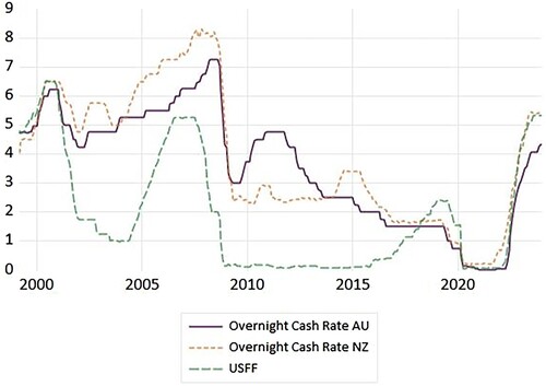
Figure 1 traces the behavior of monthly overnight cash rates in New Zealand and Australia as well as the effective federal funds rate in the United States from March 1999 to December 2023. It is evident that the level of the overnight interest rate differed from country to country at various times over the sample period. After the burst of the ‘dot.com’ bubble in the early 2000s, the federal funds rate dropped to 1 percent while the overnight cash rates, while decreasing, remained at elevated levels in Oceania. A similar episode occurred in the wake of the unprecedented monetary easing in 2008 when the federal funds rate hit the zero lower bound in the United States while the overnight cash rates in Oceania remained much higher and did not fall below 2 percent until 2016. However, it is also evident that there is a considerable degree of co-movement among the three interest rates over the sample period. Co-movement in the three interest rates occurred following the economic downturn in the United States after the burst of the ‘dot.com’ bubble, in the lead-up to, during, and after the Global Financial Crisis, and then again in the lead-up to and during the Covid pandemic. Overnight interest rates started rising first in New Zealand at the end of 2021 but the Federal Reserve caught up soon and pushed rates up rapidly to unusually high levels not seen in the United States since before the Global Financial Crisis. Both Reserve Banks followed suit and by the end of 2023 had ratcheted their policy rates up to virtually the same level (RBNZ) or somewhat below (RBA) as the Federal Reserve.

Figure 1. Overnight cash rates in Oceania and the US federal funds rate: 1999m3–2023m12.

Examining simple correlations between changes in the overnight interest rates in the three countries over the sample period supports the notion that interest rates in small open economies react to interest rate changes in the center country.⁸ Table 2 shows that the correlation between short-term interest rate changes in New Zealand and the United States is positive (0.46). The relationship between short-term interest rate changes in Australia and the United States is also positive and equally tight (0.48). A basic OLS regression of changes in the overnight cash rate in both countries on changes in the federal funds rate produces coefficient estimates of 0.45 for New Zealand and 0.42 for Australia. Adding the lagged change in the overnight cash rate to the regression yields a lower estimated coefficient on US federal funds changes (0.28 for New Zealand and 0.26 for Australia) but does not eliminate its co-movement with the overnight rate.⁹

Table 2. Co-movement in overnight interest rates.

A. Correlations between changes in overnight rates: 1999:4–2023:12
	$\mathrm{\Delta }\mathrm{OC}{R}^{\mathrm{AU}}$	$\mathrm{\Delta }\mathrm{OC}{R}^{\mathrm{NZ}}$	$\mathrm{\Delta }\mathrm{FFR}$
$\mathrm{\Delta }\mathrm{OC}{R}^{\mathrm{AU}}$	1.00
$\mathrm{\Delta }\mathrm{OC}{R}^{\mathrm{NZ}}$	0.65***	1.00
	(14.7)
$\mathrm{\Delta }\mathrm{FFR}$	0.48***	0.46***	1.00
	(9.31)	(8.81)
Note: t-statistics in parentheses.
B. Regression coefficients: 1999:4–2023:12.
Regression specification	AU $(c_1)$	AU $(c_2)$	NZ $(c_1)$	NZ $(c_2)$
$\mathrm{\Delta }\mathrm{OC}{R}_t=c+c_1\mathrm{\Delta FF}{R}_t+e_t$	0.42***	–	0.45***	–
	(0.13)		(0.09)
${\overline{R}}^2$	0.22		0.21
$\mathrm{\Delta }\mathrm{OC}{R}_t=c+c_1\mathrm{\Delta FF}{R}_t+c_2\mathrm{\Delta OC}{R}_{t-1}+e_t$	0.26***	0.47***	0.28***	0.47***
	(0.1)	(0.08)	(0.06)	(0.09)
${\overline{R}}^2$	0.41		0.41

Note: t-statistics in parentheses.

Notes: HAC (Newey West) standard errors in parentheses.

*** indicates statistical significance at 1 percent level.

All estimated coefficients for the intercept are close to zero and not significant either economically or statistically. If the selection of lag length is based on BIC, the estimated coefficients on the change in the federal funds rate change only minimally.

Data (monthly):

Overnight cash rates: RBA, RBNZ

Effective federal funds rate: Fred Data Base, St. Louis Fed

Real exchange rate (New Zealand, Trade-weighted index): RBNZ

Broad real exchange rate (Australia, index): Fred Data Base, St. Louis Fed

Abbreviations: OCRⁱ = overnight cash rate j = AU (Australia), NZ (New Zealand), REXⁱ = real exchange rate j = AU, NZ, FFR = federal funds rate.

Interest rates are expressed as natural logs: log(1 + i) where i is a decimal. The real exchange rates are expressed in log form as well.

Comparing the optimal responses of the domestic interest rate to the foreign interest rate in Table 1 with the estimated coefficient responses of overnight cash rates in Australia and New Zealand to changes in the US federal funds rate in Table 2 yields a noteworthy result. The estimated coefficients vary from 0.26 to 0.45 and thus approximate the predicted optimal response in a model economy that is relatively open on the demand side $(0.2\le \gamma \le 0.4)$, has limited openness on the supply side $(b=0.1)$ and allows free capital mobility $(\varphi =-1)$ (top panel of Table 1). Varying the size of parameters measuring openness, the extent of UIP failure or the relative aversion of the central bank to inflation variability still produces optimal responses of the domestic interest rate that do not differ greatly from the empirical estimates provided the variations do not stray too far from their base values.

Conducting a similar comparison between the model-based and estimated reaction of the real exchange rate in Oceania to a change in the federal funds rate yields less sanguine results. In the top panel of Table 3, simple correlation analysis reveals a low positive association over the whole sample period between changes in the federal funds rate and real exchange rate changes in Australia (0.13) but not in New Zealand.

Table 3. The connection between changes in the US federal funds rate and real exchange rates in Oceania.

A. Correlations between changes in US federal funds rate and real exchange rates: 1999:4–2023:12
	$\mathrm{\Delta }\mathrm{RE}{X}^{\mathrm{AU}}$	$\mathrm{\Delta }\mathrm{RE}{X}^{\mathrm{NZ}}$	$\mathrm{\Delta }\mathrm{FFR}$
$\mathrm{\Delta }\mathrm{RE}{X}^{\mathrm{AU}}$	1.00
$\mathrm{\Delta }\mathrm{RE}{X}^{\mathrm{NZ}}$	0.54***	1.00
	(10.90)
$\mathrm{\Delta }\mathrm{FFR}$	0.13**	0.08	1.00
	(2.26)	(1.44)
Note: t-statistics in parentheses.
B. Correlations between changes in US federal funds rate and real exchange rates: 2008:1–2023:12
	$\mathrm{\Delta }\mathrm{RE}{X}^{\mathrm{AU}}$	$\mathrm{\Delta }\mathrm{RE}{X}^{\mathrm{NZ}}$	$\mathrm{\Delta }\mathrm{FFR}$
$\mathrm{\Delta }\mathrm{RE}{X}^{\mathrm{AU}}$	1.00
$\mathrm{\Delta }\mathrm{RE}{X}^{\mathrm{NZ}}$	0.52***	1.00
	(8.92)
$\mathrm{\Delta }\mathrm{FFR}$	0.21***	0.19***	1.00
	(2.91)	(2.62)

Note: t-statistics in parentheses.

*** (**) indicates statistical significance at 1 (5) percent level.

At first sight, the picture changes somewhat for a shorter interval that excludes the period prior to the Global Financial Crisis. According to panel B of Table 3, over the 2008–2023 subsample period, changes in the federal funds rate bear a systematic positive relationship with changes in the real exchange rate in both New Zealand and Australia. Both correlation coefficients are substantially larger now and hover around the 0.20 mark. However, owing to the complexities that characterize the relationship between real exchange rates and policy rates, simple regression analysis is unlikely to yield precise measures of the reaction of the real exchange rate in Oceania to policy changes in the United States. Firstly, the estimated OLS coefficients on the federal funds rate for both countries (not reported) may be marred by an endogeneity bias. And, secondly, instrumental variable estimation produces very different coefficient estimates (not reported) on the federal funds rate and, in general, much larger standard errors for both countries.

Thus, overall, the empirical evidence for a systematic reaction of the exchange rate in Oceania to US interest rate changes is questionable.

6. Conclusion

Nowadays financial markets are tightly linked across the globe. Policy changes by the Federal Reserve are often accompanied by adjustments in the monetary policy stance in other countries. However, observed positive co-movements between the interest rate in the country that exercises substantial control over the global financial cycle and interest rates in smaller economies do not necessarily indicate lack of monetary independence in the latter. Optimizing central banks in small open economies that allow their exchange rate to float still retain control over their policy instrument and adjust it in the best way possible to keep fluctuations in the rate of inflation and the output gap – domestic objectives – at bay. The positive co-movement between cross-border interest rates is just an outcome of an optimal policy response. Empirical evidence on interest rate changes in New Zealand and Australia in response to US interest rate changes is consistent with this view. In contrast, there is no convincing evidence for a reaction of the real exchange rates in Oceania to US interest rate changes.

Disclosure statement

No potential conflict of interest was reported by the author(s).

Data availability statement

Data are available upon request from the author or the University of Canterbury Repository.

Notes

1 The real exchange rate is defined as $q_t=p_t^f+e_t-p_t$ where $e_t$ is the nominal exchange rate (units of domestic currency per unit of foreign currency) and the two remaining variables are the domestic and foreign price level, respectively.

2 As shown by Guender (2006), the size of b > 0 depends on the relative weight (in a firm’s cost function) on the squared deviations of the current price from the optimal price and on the sensitivity of the optimal price to marginal cost. See also Monacelli (2013) for alternative ways of motivating an exchange rate channel in the Phillips curve.

3 The source of the nominal rigidity is stickiness of domestic prices. Hence the focus on stabilizing domestic inflation.

4 Update equation (4)(4) $\begin{array}{rl}& {\pi }_t^{\mathrm{CPI}}={\pi }_t+\gamma \mathrm{\Delta }{q}_t\end{array}$(4) by one period, take conditional expectations, and substitute it into the IS relation. Eliminate the real exchange rate by substituting equation (3)(3) $\begin{array}{rl}& i_t-E_t{\pi }_{t+1}-(i_t^f-E_t{\pi }_{t+1}^f)=-\varphi (E_t{q}_{t+1}-q_t)+{\epsilon }_t\end{array}$(3) into both the IS and Phillips curve relation. The augmented IS and Phillips relations serve as the two constraints in the central bank’s optimization problem.

5 We abstract from considering the role of other parameters$(\eta ,{\eta }^f,{\gamma }^f,\sigma ,\kappa )$ since they are largely peripheral to the issue at hand. These parameters are held constant throughout the analysis. The base values chosen for the parameters appear at the bottom of Table 1 and are similar to those chosen by Svensson (2000) and Guender (2006).

6 The positive correlation between $i_t$and $i_t^f$also obtains for more extreme values of the parameters. The only case where a zero or negative correlation can come about is when the intertemporal elasticity of substitution of consumption ($\sigma$) is much higher than $\eta$. This is usually ruled out (e.g. Gali 2008).

7 Even if ‘carry trade‘ characterizes equation (3)(3) $\begin{array}{rl}& i_t-E_t{\pi }_{t+1}-(i_t^f-E_t{\pi }_{t+1}^f)=-\varphi (E_t{q}_{t+1}-q_t)+{\epsilon }_t\end{array}$(3) , i.e. $\varphi >0$, the correlation between $i_t$and $i_t^f$remains positive. Indeed, it moves remarkably close to 1. The positive correlation also holds if the mandate of the central bank expands to include a financial stability objective. See Froyen and Guender (2022).

8 Tests for non-stationarity of the three interest rates and the two real exchange rate series over the sample period were carried out at the outset. Augmented Dickey-Fuller tests could not reject the null-hypothesis of a unit root in the (level of) the time series data. Residual-based tests for cointegration (Engle-Granger and Phillips-Ouliaris) did not reject the null hypothesis of no cointegration between the three interest rates. This finding supports the notion that there is no error correction mechanism in place that forces the change in the domestic short-term interest rate to be such that it is consistent with restoring the long-run relationship with its foreign counterpart.

9 A word of caution is in order here. The changes in the three interest rates do not follow a normal distribution. This makes using the p-values for tests of significance of simple linear correlation coefficients problematic. A Spearman non-parametric test for correlation yields slightly lower positive correlations between the overnight rates than the standard (Pearson) test for linear correlation. In addition, the residuals in the reported regressions are not normally distributed. The reported coefficient estimates should therefore be interpreted with care. Despite these limitations, these estimates are still useful because they approximate the degree of co-movement between the interest rates.

10 The Federal Reserve Open Market Committee and the Monetary Policy Committee of the Reserve Bank of New Zealand meet every six weeks. The Board of the Reserve Bank of Australia meets every month except in January to decide on the monetary policy stance.

Appendix: A brief synopsis of monetary policy changes in the US and Oceania in the recent past

In the lead-up to the Global Financial Crisis, the overnight cash rates in both New Zealand and Australia followed the upward trend set by the Federal Reserve for the benchmark of US short-term interest rates. Both Reserve Banks also started to decrease rates rapidly once the Federal Reserve signaled prolonged easy monetary conditions through its announcements and purchases of long-term assets in December 2008. The zero lower bound remained in force in the United States until December 2015. By contrast, up and down movements in overnight interest rates were rather frequent in Oceania not least because the zero lower bound did not act as a constraint on monetary policy. A series of policy tightenings occurred in the United States following the first increase in the federal funds rate since 2006 in December 2015. Monetary policy followed a very different course in Oceania around the same time with monetary conditions easing in both countries at first before settling at 1.50 percent in Australia and around 1.70 percent in New Zealand.

Monetary conditions began to tighten markedly in the United States in December 2017 while policy was on hold in Oceania. In 2019 policy settings in all three countries eased. In 2020 another global crisis emerged with the outbreak of the Covid Pandemic. The Federal Reserve lowered the federal funds rate by 150 basis points over the span of two weeks in March 2020 to reach the zero lower bound again in the following month. The Reserve Banks in Oceania followed suit with the respective cash rates hitting the effective zero lower bound (<25 basis points) roughly at the same time (Australia) or shortly after (New Zealand). When unusually high inflation became a serious problem for policymakers in the three countries, monetary policy began to tighten.

Here it is instructive to take a closer look at monetary policy decisions in the three countries in 2022. Table A1 shows the policy settings at various points in time (roughly quarterly intervals). It then presents a breakdown of all adjustments in the targets for the policy rates for 2022. There were seven increases in the respective policy rate target in the United States and New Zealand and eight increases in Australia.¹⁰ The Federal Reserve acted as a pace setter, increasing the federal funds rate target by 4.25 percentage points, followed by the Reserve Bank of New Zealand’s increase of the official cash rate target of 3.5 percentage points and the cash rate target in Australia by 3 percentage points. The Reserve Bank of New Zealand was first to tighten monetary policy but did so more cautiously than the Federal Reserve. The latter increased its federal funds rate target by 75 basis points four times in a row compared to the single 75 basis point increase by the former. The Reserve Bank of Australia’s tightening cycle began later and was most intense over the June-September period when the cash target increased by 2 percentage points in four 50 basis point increments.

Table A1. Monetary policy settings in the three countries in 2022: targets for the policy rate.

New Zealand		United States		Australia
23 February	1.0%*	17 March	0.25–0.5%*	2 March	0.10%
25 May	2.0%	16 June	1.50–1.75%	8 June	0.85%
17 August	3.0%	2 September	3.00–3.24%	7 September	2.35%
23 November	4.25%	14 December	4.25–4.5%	7 December	3.10%
1x 75 basis point increase		4x 75 basis point increases		0x 75 basis point increase
5x 50 basis point increases		2x 50 basis point increases		4x 50 basis point increases
1x 25 basis point increase		1x 25 basis point increase		4x 25 basis point increases
Total increase in 2022	3.5%	Total increase in 2022	4.25%	Total increase in 2022	3%

An asterisk (*) denotes a 25 basis point increase in target rate from previous setting.

References

- Froyen, R.T., & Guender, A.V. (2022). The Mundellian Trilemma and optimal monetary policy in a world of high capital mobility. Open Economies Review, 33, 631–656.
- Gali, J. (2008). Monetary policy, inflation, and the business cycle. Princeton: Princeton University Press.
- Guender, A. (2006). Stabilizing properties of discretionary monetary policies in a small open economy. Economic Journal, 116, 309–326.
- Jeanne, O. (2022). Rounding the corners of the Trilemma: A simple framework. Journal of International Money and Finance, 122, 102551.
- Monacelli, T. (2013). Is monetary policy fundamentally different in an open economy. IMF Economic Review, 61, 6–21.
- Nelson, E. (2020). The continuing validity of monetary autonomy under floating exchange rates. International Journal of Central Banking, 16, 81–124.
- Obstfeld, M. (2021). Trilemmas and tradeoffs: Living with financial globalization. In S. J. Davis, E. S. Robinson, & B. Yeung (Eds.), The Asian monetary policy forum: Insights for central banking (pp. 16–84). Singapore: World Scientific Publishing.
- Rey, H. (2016). International channels of transmission of monetary policy and the Mundellian Trilemma. IMF Economic Review, 64, 6–35.
- Svensson, L. (2000). Open economy inflation targeting. Journal of International Economics, 50, 117–153.