
 ?Mathematical formulae have been encoded as MathML and are displayed in this HTML version using MathJax in order to improve their display. Uncheck the box to turn MathJax off. This feature requires Javascript. Click on a formula to zoom.
Abstract
Inspired by Schmidt’s work on twisted cubics, we study wall crossings in Bridgeland stability, starting with the Hilbert scheme parametrizing pairs of skew lines and plane conics union a point. We find two walls. Each wall crossing corresponds to a contraction of a divisor in the moduli space and the contracted space remains smooth. Building on work by Chen–Coskun–Nollet, we moreover prove that the contractions are K-negative extremal in the sense of Mori theory and so the moduli spaces are projective.
2020 MATHEMATICS SUBJECT CLASSIFICATION:
1 Introduction
After the introduction of Bridgeland’s manifold of stability conditions on a triangulated category [Citation6], several applications to the study of the birational geometry of moduli spaces have appeared: the moduli space is viewed as parameterizing stable objects in the derived category of some underlying variety X, and the question is how the moduli space changes as the stability condition varies. This is the topic of wall crossing in the stability manifold. We refer to [Citation15] for an overview and in particular for examples of the success of this viewpoint in cases where X is a surface. For threefolds and notably in the case , important progress was made by Schmidt [Citation20], allowing among other things a study of wall crossings for the Hilbert scheme of twisted cubics (see also Xia [Citation22] for further work on this case; additional examples in the same spirit have been investigated by Gallardo–Lozano Huerta–Schmidt [Citation11] and Rezaee [Citation19]). The case considered in the present text is that of pairs of skew lines in
and their deformations. This is analogous to twisted cubics in the sense that a twisted cubic degenerates to a plane nodal curve with an embedded point much as a pair of skew lines degenerates to a pair of lines in a plane together with an embedded point.
More precisely we study wall crossing for the Hilbert scheme of subschemes
with Hilbert polynomial
. It has two smooth components
and
: a general point in
is a conic-union-a-point
and a general point in
is a pair of skew lines
. Note that when a line pair is deformed until the two lines meet, the result is a pair of intersecting lines with an embedded point at the intersection, and this can also be viewed as a degenerate case of a conic union a point.
For an appropriately chosen Bridgeland stability condition on the bounded derived category of coherent sheaves , the ideal sheaves
can be viewed as the stable objects with fixed Chern character, say
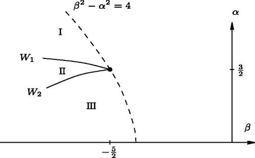
. When deforming the stability condition, we identify two walls, separating three chambers. Getting slightly ahead of ourselves, the situation is illustrated in in Section 3.2: α and β are parameters for the stability conditions considered and we restrict ourselves to the region to the immediate left in the picture of the hyperbola
(the role of this boundary curve is explained in Section 2.4). In this region we have the two walls W1 and W2 separating three chambers, labeled by Roman numerals as in the figure. Let
, and
be the moduli spaces of Bridgeland stable objects with Chern character v in each chamber, considered as algebraic spaces (for existence see Piyaratne–Toda [Citation18, Corollary 4.23]).
Our first main result contains the set-theoretical description of these moduli spaces:
Theorem 1.1.
is
Ideal sheaves
Non-split extensions
for
Ideal sheaves
Non-split extensions
with P and V as above. Moreover,
To locate walls and classify stable objects we employ the method due to Schmidt [Citation20], which involves “lifting” walls from an intermediate notion of tilt stability. Schmidt considers as an application the Hilbert scheme : it parameterizes twisted cubics and plane cubics union a point. This was our starting point and we can apply many of Schmidt’s results directly, although modified or new arguments are needed as well. The end result is closely analogous in the two cases, with two wall crossings of the same nature. In the twisted cubic situation, however, Schmidt also finds an additional “final wall crossing” where all objects are destabilized. This has no direct analogy in our case.
Next we describe the moduli spaces geometrically, guided by the set theoretic classification of objects above; this leads to contractions of the two smooth components and
of
. First introduce notation for the loci that are destabilized by the two wall crossings according to the above classification:
Notation 1.2.
Let
Let
Thus the locus (II)(i) is and the locus (III)(i) is
. On the other hand both loci (II)(ii) and (III)(ii) are parameterized by the incidence variety
consisting of pairs (P, V) of points
inside a plane
. The process of replacing E and F by I can be realized as contractions of algebraic spaces: E and F may be viewed as projective bundles over I, and in Section 4 we apply Artin’s contractibility criterion to obtain smooth algebraic spaces
and
each containing the incidence variety I as a closed subspace, and birational morphisms
which are isomorphisms outside of E, respectively F, and restrict to the natural maps
, respectively
. Moreover
is disjoint from
, so the union
makes sense as the gluing together of
and
. We can then state our second main result:
Theorem 1.3.
To prove the theorem it suffices to treat the contracted spaces as algebraic spaces. However, they turn out to be projective varieties: the contractions are in fact K-negative extremal contractions in the sense of Mori theory. The case of can be found in previous work by Chen–Coskun–Nollet [Citation8] and in fact it turns out that
is a Grassmannian; see Section 4.2. Inspired by this work, we exhibit in Section 5 the map
as a K-negative extremal contraction. This may be contrasted with Schmidt’s approach in the twisted cubic situation [Citation20], where projectivity of the moduli spaces is proved by viewing them as moduli of quiver representations.
In Section 2, we list the background results that we need, in particular, we briefly recall the construction of stability conditions on threefolds, along with the notion of tilt-stability. In Section 3 we apply Schmidt’s machinery to prove Theorem 1.1. In Section 4 we study universal families and prove Theorem 1.3. Finally, in Section 5 we work out the Mori cone of .
We work over . Throughout and in particular in Section 4, intersections and unions of subschemes are defined by the sum and intersection of ideals, respectively, and inclusions and equalities between subschemes are meant in the scheme theoretic sense. The relative ideal of an inclusion
of two closed subschemes of some ambient scheme is the ideal
defining Z as a subscheme of Y.
2 Preliminaries
After detailing the two components of , we collect notions and results from the literature surrounding Bridgeland stability and wall crossings for smooth projective threefolds. There are no original results in this section.
2.1 The Hilbert scheme and its two components
It is known that has two smooth components
and
, whose general points are conics union a point and pairs of skew lines, respectively. A quick parameter count yields
and
. We refer to Lee [Citation13] for an overview, to Chen–Nollet [Citation9] for the smoothness of
and to Chen–Coskun–Nollet [Citation8] for the smoothness of
. In fact, the referenced works show that
is the blowup
along the universal conic and
is the blowup
along the diagonal in the symmetric square of the Grassmannian G(2, 4) of lines in
. In other words, it is the Hilbert scheme
of finite subschemes in G(2, 4) of length two.
We pause to make some preparations regarding embedded points: by a curve with an embedded point at
we mean a subscheme
such that
and the relative ideal
is isomorphic to k(P). This makes sense even when we allow C to be singular or nonreduced. Embedded points are in bijection with normal directions, i.e. lines in the normal space to
at P: explicitly in our situation, suppose that
in local affine coordinates x, y, z, and C is a conic defined by the ideal
, where q is a quadric vanishing at the origin. A normal vector to C may be viewed as a k-linear map
given by say
and
. Thus
parameterizes normal directions and the corresponding scheme Y with an embedded point at P is defined by the kernel of the induced map
, which is
Example 2.1.
With notation as above, consider the degenerate conic defined by . When
we obtain the planar scheme Y in the xy-plane given by
where the final form exhibits Y as the scheme theoretic union of a pair of lines and a thickening of the origin in the xy-plane. At the other extreme
we obtain
which we label spatial: the subscheme
is not contained in any nonsingular surface since it contains a full first order infinitesimal neighborhood around P. It is easy to check that for the remaining values of
the corresponding scheme Y is neither planar nor spatial. Analogous observations hold for the double line
.
With these preparations, we next list all elements , including degenerate cases. We follow Lee [Citation13, Section 3.5], to which we refer for further details and proof that the following list is exhaustive.
The component parameterizes subschemes Y of the following form: let C be a conic in a plane
, possibly a union of two lines or a planar double line. Then Y is either the disjoint union of C and a point
, or C with an embedded point at
. If C is nonsingular at P, embedded points correspond to normal directions, parameterized by a
. Since even degenerate conics are complete intersections, also embedded point structures at a singular or nonreduced point P form a
as in Example 2.1, and among these exactly one is planar (Y contained in a plane) and exactly one is spatial (Y contains the first order infinitesimal neighborhood of P in
).
The component parameterizes pairs
of skew lines, together with its degenerations. These are of the following three types: (1) a pair of incident lines
with a spatial embedded point at the intersection point, (2) a planar double line with a spatial embedded point, or (3) a double line in a quadric surface, i.e. there is a line L in a nonsingular quadric surface Q such that Y is the effective divisor
, but viewed as a subscheme of
. We label this case the pure double line, where purity refers to the lack of embedded components.
Clearly, then, consists of the incident or planar double lines with a spatial embedded point.
2.2 Stability conditions and walls
Let X be a smooth projective threefold over and fix a finite rank lattice Λ equipped with a homomorphism
from the Grothendieck group of coherent sheaves modulo short exact sequences. On
we will take
equipped with the Chern character map
.
Recall [Citation4–6] that a Bridgeland stability condition on X (with respect to Λ) consists of
an abelian subcategory
a stability function Z, which is a group homomorphism
whose value on any nonzero object
This is subject to a list of axioms which we will not give (see [Citation4, Section 8]). We may then partially order the nonzero objects in by their slope
This yields a notion of σ-stability and σ-semistability for objects in in the usual way by comparing the slope of an object with that of its sub- or quotient objects. These notions extend to
by shifting in the sense of triangulated categories.
Bridgeland’s result [Citation6, Theorem 1.2] gives the set of stability conditions the structure of a complex manifold, and for a given
, it admits a wall and chamber structure: if an object
goes from being stable to being unstable as the stability condition σ varies, σ has to pass through a stability condition for which
is strictly semistable. This observation leads to the definition of a wall:
Definition 2.2.
Fix .
Numerical walls: A numerical wall is a nontrivial proper solution set
where
Actual walls: Let
in
When the context is clear, we drop the word “actual” and just say “wall”.
Given a union of walls, we refer to each connected component of its complement in as a chamber. By the arguments in [Citation7, Section 9] there is a locally finite collection of (actual) walls in
, each being a closed codimension one manifold with boundary, such that the set of stable objects in
with class
remains constant within each chamber, and there are no strictly semistable objects in a chamber.
We say that a short exact sequence as in (ii) above defines the wall. Relaxing this, an unordered pair defines the wall if there is a short exact sequence in either direction (i.e. we allow the roles of sub and quotient objects to be swapped) as in (ii). Semistability of
and
is automatic, i.e. it follows from semistability of
and the equality between slopes, but see Remark 2.4.
Remark 2.3.
A very weak stability condition is a weakening of the above concept (see Piyaratne–Toda [Citation18]) where Z is allowed to map nonzero objects in
to zero. One may define an associated slope function λ as before, with the convention that
also when
. An object
is declared to be stable if every nontrivial subobject
satisfies
, and semistable when nonstrict inequality is allowed. With this definition one avoids the need to treat cases where
or
separately. We will not need to go into detail.
2.3 Construction of stability conditions on threefolds
We next recall the “double tilt” construction of stability conditions by Bayer–Macrì–Toda [Citation5]. For this it is necessary to assume that the threefold X satisfies a certain “Bogomolov inequality” type condition [Citation4, Conjecture 4.1]), which is known in several cases including [Citation14]. Fix a polarization H on X; on
this will be a (hyper)plane.
2.3.1 Slope stability
Let . The twisted Chern character of a sheaf or a complex
on X is defined by
. Its homogeneous components are
The twisted slope stability function on the abelian category of coherent sheaves is given by
(2.1)
(2.1)
This is the slope of a very weak stability condition. Notice that , where
is the classical slope stability function. A sheaf
which is (semi)stable with respect to this very weak stability condition is called
-(semi)stable (or slope (semi)stable).
2.3.2 Tilt stability
Next, define the following full subcategories of
The pair is a torsion pair [Citation7, Definition 3.2] in
. Tilt the category
with respect to this torsion pair and denote the obtained heart by
. Thus every object
fits in a short exact sequence
(2.2)
(2.2) with
and
.
Let , and let
(2.3)
(2.3)
The associated slope function is
(see [Citation15, Section 9.1] for more details).
By [Proposition B.2 (case )], the pair
is a very weak stability condition continuously parameterized by
. An object
which is (semi)stable with respect to this very weak stability condition is called
-(semi)stable (or tilt (semi)stable). Moreover the parameter space
admits a wall and chamber structure [Citation4, Proposition B.5], in which walls are nested semicircles centered on the β-axis, or vertical lines (we view α as the vertical axis) [Citation20, Theorem 3.3], and a numerical wall is either an actual wall everywhere or nowhere. We refer to them as “tilt-stability walls” or “ν-walls” interchangeably.
Remark 2.4.
Walls in the parameter space for tilt stability are defined analogously to Definition 2.2. With tilt-stability in mind we make the following observation: let be strictly semistable with respect to a very weak stability condition
. By definition this means that
is semistable and there exists a short exact sequence
in
such that all three objects share the same slope. This implies that
is semistable, since any destabilizing subobject of
would also destabilize
. When very weak stability conditions are allowed, however,
may not be semistable: this happens exactly when
has finite slope and there is a nontrivial subobject
such that
. In this case let
be the maximal such subobject: then
is semistable (it is in fact the final factor in the Harder–Narasimhan filtration of
) and has the same slope as
. Moreover the kernel
of the composite
has the same slope as
. Thus in the short exact sequence
all objects are semistable and of the same slope. So when looking for walls we may as in Definition 2.2 assume all objects in the defining short exact sequence to be semistable, even in the very weak situation.
The following is the Bogomolov inequality for tilt-stability:
Proposition 2.5.
[Citation5, Corollary 7.3.2] Any -semistable object
satisfies
2.3.3 Bridgeland stability
Define the following full subcategories of :
They form a torsion pair. Tilting with respect to this pair yields stability conditions
([Citation4, Theorem 8.6, Lemma 8.8]) on X, where
and
(2.4)
(2.4)
The slope function of is given by
with
when
.
An object which is (semi)stable with respect to this stability condition is called
-(semi)stable.
The stability conditions are continuously parameterized by
[Citation4, Proposition 8.10]. We refer to walls in
as “λ-walls”.
The following lemma allows us to identify moduli spaces of slope-stable sheaves with moduli spaces of tilt-stable sheaves, given the right conditions:
Lemma 2.6.
[Citation11, Lemma 1.4] On , let
satisfy
and assume (v0, v1) is primitive. Then an object
with
is
-stable for all
if and only if
is a slope stable sheaf.
2.4 Comparison between ν-stability and λ-stability—after Schmidt
Let be an object in
. Throughout this section, let
satisfy
, and fix s > 0. We shall summarize a series of results by Schmidt [Citation20] enabling us to compare walls and chambers with respect to ν-stability with those of λ-stability. (Looking ahead to our application illustrated in and , the dashed hyperbola is the solution set to
.)
Fig. 1 The unique semicircular wall W (solid) for ν-stability and the hyperbola (dashed) from EquationEquation (3.3)(3.3)
(3.3) .
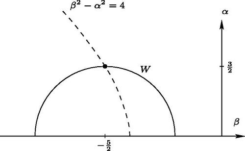
Fig. 2 The two walls W1 and W2 (solid) for λ-stability separating three chambers, together with the hyperbola (dashed) from EquationEquation (3.3)(3.3)
(3.3) .
Consider the following conditions on :
Obviously there are implications (1) (4) and (2)
(3). The following says that, under a mild condition on
, there are in fact implications
so that λ-stability in a certain sense refines ν-stability:
Theorem 2.7
(Schmidt). The implication above always holds. If
then also the implication
holds.
For the proof we refer to Schmidt [Citation20]: the first implication follows from Lemma 6.2 in loc. cit. and the second follows from Lemmas 6.3 and 6.4 (in the reference the additional condition appears; this is harmless but redundant as it is not used in the proof).
Schmidt furthermore compares walls for ν-stability and λ-stability, for objects in some fixed class
. Let
(2.5)
(2.5) be a triangle in
with
in class v.
Say that (2.5) defines a ν-wall through
Say that (2.5) defines a λ-wall at the ν-positive side of
Note that the assumption that are all in
or in
implies that the triangle (2.5) is a short exact sequence
in that abelian category.
Theorem 2.8
(Schmidt). Let be an object in
and let
such that
and
.
If a triangle (2.5) defines a λ-wall on the ν-positive side of
Suppose a triangle (2.5) defines a ν-wall through
and suppose there are points
For the proof we refer to Schmidt [Citation20]: part (1) is Schmidt’s theorem 6.1(1) and part (2) is the special case n = 1 of Schmidt’s theorem 6.1(4). To align the notation, in part (1) Schmidt’s are our
. To apply theorem 6.1(1) these are required to be
-semistable objects in
; this is ensured by Schmidt’s lemma 6.3.
To control how the set of stable objects changes as a λ-wall is crossed, we take advantage of the fact that the λ-walls we obtain are defined by short exact sequences with stable sub- and quotient objects (in other words, only two Jordan–Hölder factors on the wall) and apply:
Proposition 2.9.
Suppose and
are
-stable objects in
. Then there is a neighborhood U of
such that for all
and all nonsplit extensions
the object
is
-stable if and only if
.
This result is stated and proved (for arbitrary Bridgeland stability conditions) in Schmidt [Citation20, Lemma 3.11], and credited there also to Bayer–Macrì [Citation3, Lemma 5.9].
3 Wall and chamber structure
The starting point for the entire discussion that follows is a simple minded observation. Namely, let be a plane and let Y be the union of a conic in V and a point P also in V. Then there is a short exact sequence
(3.1)
(3.1)
(read as the ideal of V and
as the relative ideal of
). If we instead let Y be the union of a conic in V and a point P outside of V then there is a short exact sequence
(3.2)
(3.2)
(read as the ideal of
and
as the relative ideal of a conic in V). The claim is that in a certain region of the stability manifold of
, there are exactly two walls with respect to the Chern character
, and they are defined precisely by the two pairs of sub and quotient objects appearing in the short exact sequences (3.1) and (3.2).
Mimicking Schmidt’s work for twisted cubics (and their deformations), we argue via tilt stability. Since -stability only involves Chern classes of codimension at least one, and the above two short exact sequences are indistinguishable in codimension one, they give rise to one and the same wall in the tilt stability parameter space. Making this precise is the content of Section 3.1. Moving on to
-stability, we apply Schmidt’s method to see that the single
-wall “sprouts” two distinct
-walls corresponding to (3.1) and (3.2). This is carried out in Section 3.2.
3.1 ν-stability wall
Throughout we specialize to with H a (hyper)plane. Let
be the Chern character of ideal sheaves
of subschemes
.
For we have the tilted abelian category
and the slope function
. We concentrate on the region
, in which any ideal
of a subscheme
of dimension
satisfies
As is μ-stable also
for every quotient
and so
. In particular
.
We begin by establishing that there is exactly one tilt-stability wall in the region . The result as well as the argument is analogous to the analysis for twisted cubics by Schmidt [Citation20, Theorem 5.3], except that twisted cubics come with a second wall that destabilizes all objects—for our skew lines there is no such final wall.
Proposition 3.1.
There is exactly one tilt-stability wall for objects with Chern character in the region
: it is the semicircle
The wall is defined by exactly the unordered pairs of the following two types:
Moreover, the four sheaves figuring in the above unordered pairs are
The wall W and the hyperbola , intersecting at
, are shown in . Note that we visualize the α-axis as the vertical one.
We first prove the final claim in the proposition. Here is a slightly more general statement:
Lemma 3.2.
Let
Let
Remark 3.3.
The condition on in part (2) is necessary because of a wall for
. For simplicity let Z be empty. There is a short exact sequence of coherent sheaves
which yields a short exact sequence
in when
. The condition
is exactly the inequality in (2).
Proof of Lemma 3.2.
The sheaf is μ-stable and satisfies
. For all
it is thus an object in
and so also in
. Since
is a torsion sheaf it too belongs to
and so to
, for all β.
We reduce to the situation . First consider
and assume
. Note that
is a subobject of
also in
since the torsion sheaf
belongs to that category and hence
is a short exact sequence in
. Suppose
is
-stable. Let
be a proper nonzero subobject in
with quotient
. View
also as a subobject of
, with quotient
. Then
cannot distinguish between
and
. Thus if
is
-stable then
and so
is
-stable as well. The reduction from
to
is completely analogous.
-stability of the line bundle
is a consequence of
, by [Citation5, Proposition 7.4.1].
The main task is to establish -stability of
in the region defined in part (2). By point (3) of [Citation20, Theorem 3.3], the ray
intersects all potential semicircular ν-walls for
at their top point, meaning they must be centered at
. All such semicircles of radius bigger than
will intersect the ray
(as well as
). Thus it suffices to prove that
is
-stable for all
and all integers β.
For such , suppose
is a short exact sequence in
with
. We claim that
. This yields the result, since then
and so
is
-stable.
Let and
, i.e. the rank and first Chern class considered as integers. Also let
and
. By the short exact sequence we have
The induced long exact cohomology sequence of sheaves shows that , so from the short exact sequence
we see that
is a coherent sheaf in
. The remaining long exact sequence is
The map into cannot be an isomorphism, since
is in
and
is in
and is nonzero by assumption. Therefore the map in the middle is nonzero and so the rightmost sheaf
is a proper quotient of
and so is a torsion sheaf supported in dimension
. Thus only
contributes to
and
.
Suppose . As
and
we have
and since is negative we get
. Since these are integers we must have
. Thus
as claimed.
If on the other hand then also
has rank zero and hence must be zero as there are no torsion sheaves in
. Thus also
is a sheaf, with vanishing rank and first Chern class. Again
as claimed. This completes the proof. □
By explicit computation (see [Citation20, Theorem 3.3]), all numerical tilt walls with respect to in the region
are nested semicircles. More precisely, each is centered on the axis α = 0 and has top point on the curve
, that is the hyperbola
(3.3)
(3.3)
In particular every tilt wall must intersect the ray .
We establish in the following lemma that there is at most one tilt stability wall intersecting the ray for Chern character v and
. We also give the possible Chern characters of sub- and quotient objects that define it. This lemma is tightly analogous to Schmidt [Citation20, Lemma 5.5]. We use an asterisk
to denote an unspecified numerical value.
Lemma 3.4.
Let and let
be arbitrary. Suppose there is a short exact sequence
of
-semistable objects in
with
and
. Then
or the other way around.
Proof.
Keep throughout. We compute
. Let
with
and
. Then
.
Since the (very weak) stability function sends effective classes to the upper half plane
and
we have
Since this gives
.
If c = 0 then and
, which is a contradiction. Similarly if c = 2 then
and
, again a contradiction. Therefore c = 1.
With c = 1 we compute
and so the condition
says
(3.4)
(3.4)
so this expression must be strictly positive.
Suppose and apply the Bogomolov inequality (Proposition 2.5) to
:
When this gives
. On the other hand the positivity of (3.4) gives d > 0 and as d is a half integer this leaves only the possibility
and r = 1.
Similarly suppose and apply the Bogomolov inequality to
:
When this gives
. On the other hand the positivity of (3.4) gives d < 0 and as d is a half integer this leaves only the possibility
and r = 0. □
Proof of Proposition 3.1.
Assume there is a tilt stability wall for , i.e. there is a short exact sequence
of
-semistable objects in
with
and
. As already pointed out, the same conditions then hold for some
with
. Then by Lemma 3.4, up to swapping
and
, we have
(3.5)
(3.5)
(3.6)
(3.6)
Given any pair of such objects, write out the condition
on
to obtain the equation for the wall in question; this yields the semicircle as claimed. Thus we have proved that there is at most one tilt-wall and found its equation.
A further result of Schmidt [Citation20, Lemma 5.4] (which requires β to be integral, and so applies for ) says that the only
-semistable objects in
with the invariants (3.5) and (3.6) are
for a finite subscheme
, a plane
and a finite subscheme
(where Z and
are allowed to be empty). Let n and
denote the lengths of Z and
, respectively. Again for
we compute
and moreover . Thus from
we find
and so either Z is empty and
is a point, or Z is a point and
is empty. This proves that only the two listed pairs of semistable objects
may occur in a short exact sequence defining the wall.
To finish the proof it only remains to show that both pairs of objects listed do in fact realize the wall. By Lemma 3.2, the sheaves and
are in
and are
-semistable (in fact
-stable) for all
on the semicircle. Also, the ideal
of any
is an object in
(when
) and since any ideal is μ-stable it is
-stable for
(by Proposition 2.6). Hence it is
-stable outside the semicircle and at least
-semistable on the semicircle. Thus, short exact sequences of the types (3.1) and (3.2) define the wall and we are done. □
3.2 λ-stability walls
Next we apply Schmidt’s Theorem 2.8 to the single -wall found in Proposition 3.1; this yields two
-walls.
We set up notation first: for we have the doubly tilted category
and the slope function
. Once and for all we fix an arbitrary value s > 0 and view the
-plane
as parameterizing both
-stability and
-stability; as before we restrict to
. Walls and chambers are taken with respect to the Chern character
.
Write for the open subset defined by
and
; this is the region to the left of the hyperbola (3.3) in . Theorem 2.8 addresses walls in Pv close to the boundary hyperbola.
Proposition 3.5.
There are exactly two -walls with respect to
in Pv whose closure intersect the hyperbola (3.3). They are defined exactly by the two pairs of objects listed in Proposition 3.1.
This means that the two walls are
(3.7)
(3.7) and
(3.8)
(3.8)
and the pair of objects defining each wall (close to
) is unique.
We refrain from writing out the (quartic) equations defining them. They do depend on s, but independently of s they both intersect the hyperbola (3.3) in and as we will show in the following proof, W1 has negative slope at
whereas W2 has positive slope there. Thus W1 lies above W2 (α bigger) in the intersection between Pv and a small open neighborhood of
.
Proof.
We apply Schmidt’s theorem 2.8. Firstly, when we have
so the theorem applies. The first part of the theorem says that any λ-wall in Pv, having a point
with
in its closure, must be defined by one of the two pairs
listed in Proposition 3.1. This leaves W1 and W2 as the only candidates. Moreover the sub- and quotient objects
and
appearing are
-stable by Lemma 3.2. Thus the second part of the theorem says that conversely, W1 and W2 are indeed λ-walls, provided they contain points
arbitrarily close to
such that
and
. It remains to check this last condition.
So let be one of the pairs
or
. The region Pv is bounded by the hyperbola
and implicit differentiation readily shows that this has slope
at
. Similarly
has slope –1 and
is just the line
, and in each case
is the region to the left of these boundary curves. Thus it suffices to show that our walls have slope
at
. Now each wall Wi is defined by the condition
, which is equivalent to
(3.9)
(3.9) where
is the stability function defined in (2.4) from Section 2.3. Implicit differentiation of this equation at
gives, after some work, that W1 has slope
(3.10)
(3.10)
and W2 has slope
(3.11)
(3.11)
both of which are
, and we are done. □
We are now in position to prove Theorem 1.1. By Proposition 3.5 there exists an open (connected) neighborhood around the
branch of the hyperbola (3.3), such that the only λ-walls in
are W1 and W2, defined in (3.7) and (3.8). Moreover it follows from the slopes (3.10) and (3.11) that, after shrinking N further if necessary, W1 lies above (α bigger) W2 throughout
. Thus the two walls separate N into three chambers, which we label I, II, and III in order of decreasing α.
Proof of Theorem 1.1
(I). By Proposition 3.1 there is a single semicircular wall (in the region ) for ν-stability. It follows from Theorem 2.7 that the class of
-stable objects in
for
in chamber I coincides with the class of
-stable objects in
for
outside the single ν-wall (up to shrinking N even further if necessary).
Moreover, for α sufficiently big, the ν-stable objects in are exactly the μ-stable coherent sheaves (Proposition 2.6). For Chern character
these are the ideals
with
. □
Proof of Theorem 1.1
(II). Let be
-stable for
in chamber II. Since semistability is a closed property,
is semistable on the wall W1. If
is stable on the wall, then it is also stable in chamber I hence it is an ideal sheaf in
by part (I). Such an ideal remains stable on the wall if and only if it is not an extension of the type (3.1), that is if and only if it is the ideal of a nonplanar subscheme. This is case (II)(i) in the Theorem.
If on the other hand is stable in chamber II, but strictly semistable on W1, then by Proposition 3.5 it is a nonsplit extension of the pair
(3.12)
(3.12) and we determine the direction of the extension (which object is the subobject and which is the quotient) as follows: we claim that
(3.13)
(3.13)
for all
in chamber II sufficiently close to
. Granted this, it follows that for
to be stable in chamber II it must be a nonsplit extension as in case (II)(ii) in the Theorem. Conversely it follows from Proposition 2.9 that every such nonsplit extension is indeed stable in chamber II. To verify (3.13) we let
(3.14)
(3.14)
with
and
. Thus W1 is defined by
and (3.13) is equivalent to
. It thus suffices to check that the partial derivative of
with respect to α is positive at
. An explicit computation yields in fact
It remains only to show uniqueness of the nonsplit extensions , that is
But this space is , which is isomorphic to
via the short exact sequence
□
Proof of Theorem 1.1
(III). Let be
-stable for
in chamber III. Since semistability is a closed property,
is semistable on the wall W2. If
is stable on W2, then it is stable in chamber II. This means two things: first, by part (II) of the Theorem
is either an ideal sheaf of a nonplanar subscheme or a nonsplit extension
as in case (II)(ii). Second, to remain stable on W2 the object
cannot be in a short exact sequence of the type (3.2) ruling out ideal sheaves of plane conics union a point. Also the sheaves
sit in short exact sequences of this type, as we show in Lemma 3.6 (the vertical short exact sequence in the middle), and so are ruled out as well. Hence
is an ideal sheaf of a disjoint pair of lines as claimed in (III)(i).
If on the other hand is strictly semistable on W2, then by Proposition 3.5
is a nonsplit extension (in either direction) of the pair
Now we claim that
for all
in chamber III sufficiently close to
. We prove this as in part II above, by partial differentiation of
defined in (3.14), this time with
and
. We find
As before we conclude that is a nonsplit extension as in (III)(ii) and by Proposition 2.9 all such extensions are stable.
It remains to verify uniqueness of the extensions , i.e.
when
. For this first apply
to the short exact sequence
to obtain a long exact sequence which together with the vanishing of and
gives an isomorphism
and ignoring twists, as these are not seen by k(P), the right hand side is Serre dual to
. This is one dimensional as is seen by applying
to the sequence
□
3.3 The special sheaves
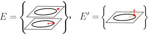
Let and
denote sheaves given by nonsplit extensions of the form (1.1) and (1.2), respectively. The definition through (unique) nonsplit extensions is indirect and it is useful to have alternative constructions available. We give such constructions here and compute the spaces of first order infinitesimal deformations.
Lemma 3.6.
There is a commutative diagram with exact rows and columns as follows:
[[INLINE FIGURE]]
Proof.
Up to identifying the skyscraper sheaf k(P) with any of its twists, there are canonical short exact sequences as in the bottom row and the rightmost column. The diagram can then be completed by letting be the fiber product as laid out by the square in the bottom right corner. It remains only to verify that the middle row is nonsplit. But if it were split the middle column twisted by
would be a short exact sequence of the form
Taking global sections this yields a contradictory left exact sequence in which all terms vanish except . □
Proposition 3.7.
We have .
Proof.
We will actually only prove that the dimension is at most 11. The opposite inequality may be shown by similar techniques, although it follows from viewing as a Zariski tangent space to the 11-dimensional moduli space
studied in the next section.
Apply to the middle row in the diagram in Lemma 3.6. This yields a long exact sequence
and from the middle column of the diagram we compute
. Thus we proceed to show that
.
Apply to the middle row in the diagram. This yields a long exact sequence:
The space on the right is Serre dual to , which again on V is Serre dual to
. This has dimension 6. At least heuristically, the space on the left should have dimension 5, as it may be viewed as a tangent space to the incidence variety
seen as a moduli space for the sheaves
. More directly we may apply
to the Koszul complex on V
to obtain a long exact sequence
where the indicated dimensions may be computed by applying
(for d = 1, 2) to the sequence
We skip further details. It follows then that and so
is at most
. □
Lemma 3.8.
There is a commutative diagram with exact rows and columns as follows:
[[INLINE FIGURE]]
Proof.
From the Euler sequence
(3.15)
(3.15) on
it follows that
has a unique section (up to scale) vanishing at
. This leads to the short exact sequence in the bottom row. Moreover there is a canonical short exact sequence as in the rightmost column. The rest of the diagram can then be formed by taking
to be the fiber product as laid out by the bottom right square. It just remains to verify that the middle row is indeed nonsplit. But if it were split the middle column would be a short exact sequence of the form
This sequence implies that is isomorphic to
, which is one dimensional. But the Euler sequence shows that in fact
. □
Proposition 3.9.
We have .
Proof.
We will be using the short exact sequence
(3.16)
(3.16) which sits as the middle column in Lemma 3.8. As preparation we observe that all (dimensions of)
may be computed from the Euler sequence, and this enables us to compute several
from (3.16). We use these results freely below without writing out further details.
Apply to (3.16) to produce a long exact sequence
in which we have indicated some of the dimensions:
are computed from (3.16) as sketched above, and since
is simple we have
. For the same reason (3.16) is nonsplit, which implies
. It thus remains to see that the dimension of
is 11.
Next apply to the Euler sequence. This gives a long exact sequence
where again dimensions have been indicated: the vanishing of
has already been noted, and there remain several spaces of the form
. These may be computed from
and the long exact sequence resulting from applying
to
It follows that and we are done. □
4 Moduli spaces and universal families
By the classification of stable objects in chamber II, the moduli space is at least obtained as a set from
by just replacing the divisor
, parameterizing conics union a point inside a plane, with the incidence variety I, parameterizing just pairs (P, V) of a point P inside a plane V. Similarly, the moduli space
of stable objects in chamber III is obtained from
set-theoretically by removing
and replacing the divisor
, parameterizing pairs of incident lines with a spatial embedded point at the intersection, with the incidence variety I. We shall carry out each of these replacements as a contraction, i.e. a blow-down, and prove that this indeed yields
and
, essentially by writing down a universal family for each case.
4.1 The contraction
Recall that is isomorphic to the blow-up of
along the universal curve
, where
is the Hilbert scheme of plane conics in
[Citation13]. The exceptional divisor
is comprised of plane conics with an embedded point.
It is helpful to keep an eye at the following diagram
[[INLINE FIGURE]] (4.1)where π sends a conic to the plane
it spans and b is the blowup along the universal family
of conics.
Remark 4.1.
It will sometimes be useful to resort to explicit computation in local coordinates. For this let be the affine open subset of planes
with equation of the form
(4.2)
(4.2)
Furthermore the of symmetric 3 × 3 matrices
parameterizes plane conics
(4.3)
(4.3) so that
with universal family defined by the two Equationequations (4.2)
(4.2)
(4.2) and Equation(4.3)
(4.3)
(4.3) . This is also the center for the blowup b, and we note that it is nonsingular.
Lemma 4.2.
π is a Zariski locally trivial -bundle. More precisely, let
be the incidence variety and let
Then is locally free of rank 6 and
over
.
Here denotes the projective bundle parameterizing lines in the fibers of
. Starting with the observation that the fiber of
over
is
(note that
, so base change in cohomology applies) the Lemma is straight forward and we refrain from writing out details.
Now let be the locus of planar
. The condition on a disjoint union
to be in E is just that P is in the plane V spanned by C. For a conic with an embedded point the condition
also singles out the scheme structure at the embedded point. View E as a variety over the incidence variety
via the morphism
(refer to for simple illustrations of the types of elements in E and
. In fact, we find it helpful for keeping track of the various divisors introduced in this section.)
Fig. 3 A Circle represents a conic contained in a plane that is shown as a parallelogram, and a red dot is a point, possibly embedded in the conic. The arrow is the direction vector at an embedded point. Note that in the left illustration, the arrow is strictly contained in the plane.
Proposition 4.3.
E is a Zariski locally trivial -bundle over the incidence variety
. The restriction
to a fiber is isomorphic to
.
Before giving the proof, we harvest our application:
Corollary 4.4.
There exist a smooth algebraic space , a morphism
and a closed embedding
, such that
restricts to an isomorphism from
to
and to the given projective bundle structure
. Moreover
is the blowup of
along I.
It is well known that the condition verified in Proposition 4.3 implies the contractibility of E/I in the above sense. In the category of analytic spaces this is the Moishezon [Citation16] or Fujiki–Nakano [Citation10, Citation17] criterion. In the category of algebraic spaces the contractibility is due to Artin [Citation2, Corollary 6.11], although the statement there lacks the identification with a blowup. Lascu [Citation12, Théorème 1] however shows that once the contracted space as well as the image
of the contracted locus are both smooth, it does follow that the contracting morphism is a blowup. Strictly speaking Lascu works in the category of varieties, but our
turns out to be a variety anyway:
Remark 4.5.
The algebraic space is in fact a projective variety. We prove this in Section 5 using Mori theory. As the arguments there and in the present section are largely independent we separate the statements.
We also point out that the smooth contracted space is unique once it exists: in general, suppose
and
are proper birational morphisms between irreducible separated algebraic spaces (say, of finite type over k) with U and V normal. Moreover assume that
if and only if
. Let Γ denote the image of
. Then each of the projections from Γ to U and V is birational and bijective and hence an isomorphism by Zariski’s Main Theorem (for this in the language of algebraic spaces we refer to the Stacks Project [Citation21, Tag05W7]).
Proof of Proposition 4.3.
Consider the divisor
It follows from Lemma 4.2 that
is a
-bundle, hence its restriction to
is a
-bundle over
.
Now, E is the strict transform of , i.e. its blow-up along
. But this is a Cartier divisor, since
is smooth, and so
. This proves the first claim.
Again using that is smooth, its strict transform E satisfies the linear equivalence
(4.4)
(4.4)
The term is a pullback from the base of the
-bundle, so its restriction to any fiber is trivial. Thus it suffices to see that
restricted to a fiber
is a hyperplane. Now the isomorphism
identifies
with
. In the local coordinates from Remark 4.1 the divisor E is given by Equationequation (4.2)
(4.2)
(4.2) and
is given by the additional Equationequation (4.3)
(4.3)
(4.3) . Here
are the coordinates on the fiber
and clearly (4.3) defines a hyperplane in each fiber—it is the linear condition on the space of plane conics given by passage through a given point. □
Remark 4.6.
The locus consists of pairs of intersecting lines with a spatial embedded point at the intersection (and, as degenerate cases, planar double lines with a spatial embedded point). On the other hand E consists only of planar objects, so E is disjoint from
. Thus we may extend the contraction
to a morphism between algebraic spaces
which is an isomorphism away from E and restricts to the -bundle
as before.
4.2 Moduli in chamber II
In this section we shall modify the universal family on the Hilbert scheme in such a way that we replace its fibers over
with the objects
in Theorem 1.1. This family induces a morphism
and we conclude via uniqueness of normal (in this case smooth) contractions that
coincides with
.
Here is the construction: let
be the universal family and let
be the E-flat family whose fiber
over a point ξ mapping to
is the plane V. Clearly
can be written down as a pullback of the universal plane over
. We view
as a closed subscheme of
. Then our modified universal family is the ideal sheaf
.
Remark 4.7.
We emphasize the (to us, at least) unusual situation that is the ideal of a very nonflat subscheme, yet as we show below it is flat as a coherent sheaf. Its fibers over points in E are not ideals at all, but rather the objects
.
Theorem 4.8.
As above let be the universal family over
and
the family of planes in
parameterized by E.
The morphism
We begin by showing that the fibers over
sit in a short exact sequence of the type (1.1). The mechanism producing such a short exact sequence is quite general. Note that when
is a conic with a (possibly embedded) point P in a plane
, we have
and
.
Lemma 4.9.
Let X be a projective scheme, an S-flat subscheme,
a Cartier divisor and
an E-flat subscheme such that
. Let
. Then there is a short exact sequence
In particular if S is integral in a neighborhood of E then is flat over S.
Proof.
Observe that the last claim is implied by the first: outside of E the ideal agrees with
, which is flat. For
we have
and so a short exact sequence
The short exact sequence in the statement has the same sub and quotient objects in opposite roles, so the Hilbert polynomial of agrees with that of
. Thus the Hilbert polynomial of the fibers of
is constant; over an integral base this implies flatness.
Begin with the short exact sequence
and tensor with to obtain the exact sequence
(4.5)
(4.5)
The kernel of the rightmost map is clearly the ideal . To compute the Tor-sheaf on the left use the short exact sequence
Pull this back to X × S and tensor with to see that
is isomorphic to the kernel of the homomorphism
which locally is multiplication by an equation for E. Thus
where
is the ideal locally consisting of elements annihilated by an equation for E.
We compute in an open affine subset
in which
and
are given by ideals
and
respectively and
is (the pullback of) a local equation for E. Thus
corresponds to
. Now
since
. This implies that for
the condition
is equivalent to
and so
. Moreover the latter equals
, since
is flat over S, so that multiplication by the non-zero-divisor f remains injective after tensor product with
, that is
. Thus
is locally
where we write
for the restriction
. This shows
and (4.5) gives the short exact sequence
on X × E. Finally restrict to the fiber over a point
: since
and
are both E-flat this yields the short exact sequence in the statement. □
Lemma 4.9 does not guarantee that the short exact sequence obtained is nonsplit. Showing this in the case at hand requires some work. Our strategy is to exhibit a certain quotient sheaf and check that the split extension
admits no surjection onto
. In fact
will work:
Lemma 4.10.
Let be a plane and
a point. Then there is no surjection from
onto
.
Proof.
Just note that is generated by the (nonsurjective) inclusion, whereas
. □
We will produce the required quotient sheaf by the following construction, which depends on the choice of a tangent direction at ξ in S:
Lemma 4.11.
With notation as in Lemma 4.9, let and let
be a closed embedding such that
is the reduced point
. Let
and
.
Define a subscheme by the ideal
where
is the ideal of
. Then there is a surjection
Remark 4.12.
Since we trivially have
. Since also
we furthermore have
. If we extend T to an actual one parameter family of objects Yt, we may think of
as the limit of
as
, in other words it is the part of Y that remains in V as we deform along our chosen direction.
Proof.
Let denote the restriction of
to T. We claim that
is isomorphic to the relative ideal of
in
. Assuming this, there are surjections
(the middle term is the ideal of as a subscheme of
). Restriction to the fiber over ξ gives the surjection in the statement.
To prove the claim, we first observe that for any two subschemes A and B of some ambient scheme, there is an isomorphism
between the relative ideal sheaves; this is the identity
between quotients of ideals. Apply this to
so that
The claim as stated thus says that is isomorphic to
, and we are free to replace the latter by
.
Next let be an affine open subset in V and
the ideal defining
there. Locally the ideal
is then
. Now multiplication with t is an isomorphism of
-modules
The left hand side is precisely in the open subset
. □
Proof of Theorem 4.8
(i). By Lemma 4.9 it suffices to show that the fiber of over
is isomorphic to
. Moreover, for such ξ, the same Lemma yields a short exact sequence
and since
is the unique such nonsplit extension it is enough to show that the above extension is nonsplit. In view of Lemma 4.10 this follows once we can show the existence of a surjection
For this it suffices, in the notation of Lemma 4.11, to choose such that the subscheme
is a conic.
Nondegenerate case. First assume is a disjoint union
of a conic
and a point
. Consider the one parameter family
in which the conic part C is fixed while the point Pt travels along a line intersecting V in the point P. In suitable affine coordinates we may take V to be the plane z = 0 in
, the point P to be the origin and C to be given by some quadric
not vanishing at P. Let the one parameter family over
consist of the union of C with the point
. This is given by the ideal
Now restrict to and intersect the family with V × T. The resulting subscheme is defined by the ideal
and
which defines
. Thus
and we are done.
Embedded point with nonsingular support. Suppose Y is a conic with an embedded point supported at a point P in which C is nonsingular, where the normal direction corresponding to the embedded point is along V. Then take the one parameter family in which C and the supporting point P is fixed and the embedded structure varies in the
of normal directions. In suitable affine coordinates we may take V to be the plane z = 0 in
, P to be the origin and C given by a quadric
vanishing at P and with, say, linear term y. Take the one parameter family of C with an embedded point given by
(the equality requires some computation). After intersection with V × T this gives
and
. This is C.
Embedded point at a singularity. Let be the union of two distinct lines intersecting in P and consider a planar embedded point at P. Despite the singularity, there is still a
of embedded points at P. We take this to be our one parameter family, i.e. we deform the embedded point structure away from the planar one.
In local coordinates we take P to be the origin in and C to be the union of the x- and y-axes in the xy-plane V. Then
is our one parameter family of embedded points at the origin, with t = 0 corresponding to the planar embedded point. The intersection with V × T is given by
and
. This is C.
Embedded point in a double line. Let be a planar double line together with a planar embedded point at
and take the one parameter family of embedded points in P.
In local coordinates we take P to be the origin in and C to be
. Then
is our one parameter family of embedded points at the origin, with t = 0 corresponding to the planar embedded point. The intersection with V × T is given by
and . This is C. □
Proof of Theorem 4.8
(ii). The morphism is clearly an isomorphism away from E, and it sends
(lying over
) to
, which determines and is uniquely determined by (P, V). Moreover
is smooth at these points by Proposition 3.7. The claim follows from uniqueness of normal contractions. □
4.3 Moduli in chamber III
In this section we show that the moduli space is a contraction of
. The argument parallels that for
closely.
Let be as in Notation 1.2. Thus an element
is either a pair of intersecting lines with a spatial embedded point at the intersection, or as degenerate cases, a planar double line with a spatial embedded point. It is in a natural way a
-bundle over the incidence variety
via the map
that sends Y to the pair (P, V) consisting of the support
of the embedded point and the plane V containing
. In parallel with Proposition 4.3 one may show that
restricts to
in the fibers of F/I and so there is a contraction
(4.6)
(4.6)
to a smooth algebraic space
, such that ψ is an isomorphism away from F and restricts to the
-bundle
. However, in this case we can be much more concrete thanks to the work of Chen–Coskun–Nollet [Citation8], where birational models for
are studied in detail (and in greater generality: moduli spaces for pairs of codimension two linear subspaces of projective spaces in arbitrary dimension). The following proposition is [Citation8, Theorem 1.6 (4)]; we sketch a simple and slightly different argument here.
Proposition 4.13.
There is a contraction as in (4.6) where is the Grassmannian G(2, 6) of lines in
.
Proof.
First consider an arbitrary quadric . Any finite subscheme in Q of length 2, reduced or not, determines a line in
. This defines a morphism
(4.7)
(4.7)
It is clearly an isomorphism away from the locus in consisting of lines contained in Q. On the other hand, over every element of
defining a line contained in Q, the fiber is the
consisting of length two subschemes of that line.
Apply the above observation to the (Plücker) quadric in
, so that
(see Section 2.1). For every plane
and every point
, the pencil of lines in V through P defines a line in
and in fact every line is of this form. The fiber of (4.7) above such an element of G(2, 5) consists of all pairs of lines in V intersecting at P. It follows that (4.7) is the required contraction
. □
Remark 4.14.
Chen–Coskun–Nollet furthermore shows that (4.6) is a K-negative extremal contraction in the sense of Mori theory. In fact, is Fano and its Mori cone is spanned by two rays. Either ray is thus contractible; one contraction is (4.6) and the other is the natural map to the symmetric square of the Grassmannian of lines in
. This statement is extracted from Theorem 1.3, Lemma 3.2, and Proposition 3.3 in loc. cit. Inspired by this work we return to the Mori cone of the conics-with-a-point component
in Section 5.
We proceed as for chamber II by modifying the universal family of pairs of lines in order to identify the moduli space with the contracted space
. Let
be the restriction of the universal family over
to the component
. Moreover, there is a flat family over the incidence variety
whose fiber over (P, V) is the plane V with an embedded point at P. Pull this back to F to define a family
We argue as in Section 4.2 but with the family of planes replaced by the family of planes with an embedded point
.
Theorem 4.15.
Let and
be as above.
The morphism
For lying over (P, V) we have
and
. Thus Lemma 4.9 yields a short exact sequence
and we show that it is nonsplit by exhibiting a certain quotient sheaf of
. This time we use
where
is a point distinct from P.
Lemma 4.16.
Let be a plane and
two distinct points. There is no surjection from
to
.
Proof.
Every nonzero homomorphism
has image of the form where
is a line, whereas every nonzero homomorphism
has image
. Thus any nonzero homomorphism from the direct sum of these two sheaves has image
where
is one of
or their sum
Thus the image is never for
. □
Proof of Theorem 4.15.
The proof for Theorem 4.8 carries over; we only need to detail the construction of quotient sheaves via one parameter families. As before we write down families over and then restrict to
. We then apply Lemma 4.11, with
in the role of the family denoted
in the Lemma. The outcome of Lemma 4.11 will be a quotient sheaf of the form
, where
is a plane V with an embedded point at P. We end by intersecting with V to produce a further quotient of the form
. We shall choose one parameter families such that the latter is isomorphic to
with
.
Distinct lines. Let be a pair of distinct lines inside V intersecting at P. Choose another plane
containing L0 and a point
distinct from P. The pencil of lines
through Q yields a one parameter family
of disjoint pairs of lines for
, with flat limit
being C with a spatial embedded point at P.
In suitable affine coordinates let V be V(z), let P be the origin and let
. Then
. Furthermore let
and
. This leads to the family Z defined by the ideal
and the intersection with W × T is given by
Thus , which defines the union of the x-axis and the point Q. This is
and thus
is isomorphic to
.
Double lines. Let be a double line inside the plane V with
. We shall define an explicit one parameter family with central fiber
being C with a spatial embedded point at P.
Geometrically, the family is this: let be the supporting line of C. Consider a line
not through P and let Q be its intersection point with L. Also let
be a line through P and not contained in V. Let Rt be a point on M moving toward Q as
, and let
be a point on
moving toward P, but much faster than Rt moves (quadratic versus linearly). Then let Lt be the line through Rt and
and let
for
.
Let P be the origin in suitable affine coordinates , let V be the xy-plane V(z) and let
be the double x-axis
. Thus Y0 corresponds to
Now let , let Lt be the line through
and
, that is
and take
for
. This yields the family (the following identity requires a bit of fiddling)
Reducing this modulo t gives the original Y0. The intersection with W × T gives
and so
is defined by
This is the line L with an embedded point at Q (inside V) and another embedded point along the z-axis at P. Intersecting with V removes the embedded point at P, leaving the line L with an embedded point at Q. Thus .
This establishes part (i) precisely as in the proof of Theorem 4.8 and part (ii) then follows by smoothness of (from Proposition 3.9) and by uniqueness of normal (here smooth) contractions. □
5 The Mori cone of and extremal contractions
In this final section we shall prove that is the contraction of a K-negative extremal ray in the Mori cone. It follows that the contracted space
is projective.
To set the stage we recall the basic mechanism of K-negative extremal contractions. Let X be a projective normal variety and α a curve class (modulo numerical equivalence) which spans an extremal ray in the Mori cone. If also the ray is K-negative, i.e. the intersection number between α and the canonical divisor KX is negative, then there exists a unique projective normal variety Y and a birational morphism which contracts precisely the effective curves in the class α.
5.1 Statement
We denote elements in by the letter Y. It is the union of a (possibly degenerate) conic denoted C and a point denoted P. If the point is embedded,
denotes its support. We also write
for the unique plane containing C.
Define four effective curve classes (modulo numerical equivalence) on . Each is described as a family
, and we use a subscript t to indicate a parameter on the piece that varies (all choices are to be made general, e.g. C nonsingular unless stated otherwise, etc.):
δ:fix a conic C and a point . Let Yt be C with an embedded point at P, varying in the
of normal directions to
at P.
:fix a plane V, a conic
and a line
. Let Pt vary along L and let
.
:fix a plane V, a pencil of conics
and a point
. Let
.
:fix a line L and a point
. Let Vt be the pencil of planes containing L and let Ct be the planar double structure on L inside Vt. Then let Yt be Ct with an embedded spatial point at P.
In ϵ there are implicitly two elements with an embedded point, namely where L intersects C. Similarly there is one element in ζ with an embedded point, corresponding to the pencil member Ct that contains P.
Theorem 5.1.
The Mori cone of is the cone over a solid tetrahedron, with extremal rays spanned by the four curve classes
. Of these, the first three are K-negative, whereas η is K-positive. The contraction corresponding to ζ is
.
Corollary 5.2.
is projective.
Remark 5.3.
The last claim in the theorem is clear: by contracting ζ we forget the conic part of , keeping only V and the point
. By uniqueness of (normal) contractions the contracted variety is
. Also, with reference to Diagram Citation4.Citation1 (from Section 4.1), the contraction of δ is the blowing down b. The theorem furthermore reveals a third K-negative extremal ray spanned by ϵ. The corresponding contraction has the effect of forgetting the point part of
, keeping only the conic; thus the contracted locus in
is the same as for ζ, but the contraction happens in a “different direction.” We do not know if the contracted space has an interpretation as a moduli space for Bridgeland stable objects.
5.2 The canonical divisor
Use notation as in Diagram Citation4.Citation1 and Lemma 4.2. We read off that the Picard group of has rank 4 and is generated by the pullbacks of the following divisor classes:
Moreover numerical and linear equivalence of divisors coincide on . Here we only use that the Picard group of a projective bundle over some variety X is
, with the added summand generated by
, and the Picard group of a blowup of X is
, with the added summand generated by the exceptional divisor.
As long as confusion seems unlikely to occur we will continue to use the symbols H, and A for their pullbacks to
, or to an intermediate variety such as
in Diagram Citation4.Citation1.
Lemma 5.4.
The canonical divisor class of is
Proof.
This is a standard computation. First, for the blowup b, with center of codimension two, we have
and for the product
Now and for the projective bundle
we have
Again and the short exact sequence
gives
Putting this together, the stated expression for follows once we have established that
.
Recall that . We compute its first Chern class by brute force: apply Grothendieck–Riemann–Roch to
. Note that all higher direct images vanish, since
for all
and p > 0. Thus by Grothendieck–Riemann–Roch the class
is the push forward in the sense of the Chow ring of the degree 4 homogeneous part of
We have
(5.1)
(5.1)
Moreover is a divisor of bidegree (1, 1), so there is a short exact sequence
from which we see (suppressing the explicit pullbacks of cycles in the notation)
(5.2)
(5.2)
Now multiply together (5.1) and (5.2) and observe that the -coefficient is 4. Since the push forward
of any degree 4 monomial
equals
if k = 3 and 0 otherwise, this shows that
. □
5.3 Basis for 1-cycles
We will need a few more effective curves, as before written as families :
fix a conic C and a line L. Let the point Pt vary along L and let
.
fix a quadric surface
, a line L and a point P. Let Vt run through the pencil of planes containing L and let
. Then take
.
fix a plane V and a point P. Let
run through a pencil of conics and let
.
As before all choices are general, so that in the definition of α, the line L is disjoint from C, etc.
Lemma 5.5.
The dual basis to is
.
Proof.
We need to compute all the intersection numbers and verify that we get 0 or 1 as appropriate. Here it is sometimes useful to explicitly write out the pullbacks to , e.g. writing
rather than H. We view
not just as equivalence classes, but as the effective curves defined above. Only the intersection numbers involving β require some real work, and we will save this for last.
Intersections with α: Since is the line
defining α we have
. Similarly
shows that the intersections with
and A vanish. Finally α has no elements with embedded points, so is disjoint from
.
Intersections with γ: We have because γ is a line in a fiber of the projective bundle π, whereas A restricts to a hyperplane in every fiber. The remaining intersection numbers vanish as we can pick disjoint effective representatives.
Intersections with δ: We have as δ is a fiber of the blowup b and
is the exceptional divisor. The remaining divisors H,
, and A are all pullbacks, i.e. of the form
and then
.
Intersections with β: We can choose β to be disjoint from H and . Moreover
is the line
dual to the line L defining β. This gives
.
It remains to verify . The definition of β can be understood as follows: choose a general section
and apply to obtain a homomorphism
(5.3)
(5.3) whose fiber over
is exactly the restriction of σ to V. This is nowhere zero, so (5.3) is a rank 1 subbundle and it defines a section
with
or in terms of divisors
. If we let
be the quadric defined by σ then
. Thus
where
is the dual to the line L defining β. This gives
□
We also define the following three effective divisors, phrased as a condition on :
all Y whose conic part C intersects a fixed line
.
all Y such that the line through P and a fixed point
intersects the conic part C.
all planar Y (as before).
Since D is defined by a condition on C only, it is the preimage by (see Diagram Citation4.Citation1) of the similarly defined divisor in
. Moreover
and E are the strict transforms by b of the similarly defined divisors on
.
We will need to control elements of with an embedded point.
Lemma 5.6.
Fix P0 so that is defined as an effective divisor. Choose a plane V not containing P0, a possibly degenerate conic
and a point
. Then there is a unique
with conic part C and an embedded point at P. More precisely:
If C is nonsingular at P then the embedded point structure is uniquely determined by the normal direction given by the line through P0 and P.
If C is a pair of lines intersecting at P or a double line, then the embedded point is the spatial one, i.e. the scheme theoretic union of C and the first order infinitesimal neighborhood of P in
Proof.
Let Q be the cone over C with vertex P0. This is a quadratic cone in the usual sense when C is nonsingular, otherwise Q is either a pair of planes or a double plane. A disjoint union with
is clearly in
if and only if it is a subscheme of Q.
On the one hand this shows that the subschemes Y listed in (1) and (2) are indeed in , since they are obtained from
by letting
approach P along the line joining P0 and P.
On the other hand it follows that if then
, since the latter is a closed condition on Y. In case (1) Q is nonsingular at P and so there is a unique embedded point structure at
which is contained in Q. In case (2) the following explicit computation gives the result: suppose in local affine coordinates that C is the pair of lines V(xy, z), the “vertex” P0 is on the z-axis and P is the origin. Then Q is the pair of planes V(xy). Any C with an embedded point at P has ideal of the form
for
. This contains the defining equation xy of Q if and only if t = 0, which defines the spatial embedded point. The case where C is double line
is similar. □
Lemma 5.7.
We have
Proof.
The last equality was essentially established in the proof of Proposition 4.3: it follows from the observations (1) E is the strict transform of b(E), and (2) the latter is the pullback of the incidence variety which is linearly equivalent to
.
The remaining two identities are verified by computing the intersection numbers with the curves in the basis from Lemma 5.5. All curves and divisors involved are concretely defined and it is easy to find and count the intersections directly. Some care is needed to rule out intersection multiplicities, and we often find it most efficient to resort to a computation in local coordinates. We limit ourselves to writing out only two cases.
The case : As we noted D is really a divisor on
and so we shall write it here as
. Then
consists of all conics intersecting a fixed line M. We have
and
is the family of conics
where Q is a fixed quadric surface and Vt runs through the pencil of planes containing a fixed line L. For general choices
consists of two points, and each point spans together with L a plane. This yields exactly two planes V0 and V1 in the pencil for which
and
intersects M. It remains to rule out multiplicities.
In the local coordinates in Remark 4.1 let . Then the intersection between M and the plane
is the point
. Now D is the condition that this point is on C, i.e. it satisfies Equationequation (4.3)
(4.3)
(4.3) ; this gives that D is
. On the other hand,
is a one parameter family in which ci and sij are functions of degree at most 2 in the parameter. To stay concrete, let Q be
and let Vt be
. Substitute x3 = tx2 in the equation for Q to find
. This gives in particular
and so the intersection with D is indeed two distinct points, each of multiplicity 1.
The case : This is essentially Lemma 5.6, but to ascertain there is no intersection multiplicity to account for we argue differently.
is the strict transform of the divisor
, which contains the center of the blowup. Since
is nonsingular (pick
in the definition of
, then in the local coordinates of Remark 4.1 it is simply given by the Equationequation (4.3)
(4.3)
(4.3) ) we have
. Thus
and we are done.
The remaining cases are either similar to these or easier. □
5.4 Nef and Mori cones
It is clear that H, and D are base point free, hence nef. For instance, consider D: given
, choose a line
disjoint from
. This defines an effective representative for D not containing Y.
Lemma 5.8.
The divisor is nef.
Proof.
We begin by narrowing down the base locus of . First consider an element
without embedded point, that is a disjoint union
. Then choose P0 such that the line through P0 and P is disjoint from C. This defines a representative for
not containing Y, so Y is not in the base locus.
Next let Y be a conic C with an embedded point at a point where C is nonsingular. The tangent to C at P together with the normal direction given by the embedded point determines a plane. Pick P0 such that the line through P and P0 defines a normal direction to C which is distinct from that defined by the embedded point. This determines a representative for
which by Lemma 5.6(i) does not contain Y, so Y is not in the base locus.
The remaining possibility is that Y is either a pair of intersecting lines with an embedded point at the singularity, or a double line with an embedded point. Pick a representative for by choosing P0 outside the plane containing the degenerate conic. If the embedded point is not spatial, then Lemma 5.6(ii) shows that Y is not in
. So Y is not in the base locus unless the embedded point is spatial.
Thus let be the locus of intersecting lines with a spatial embedded point at the origin, together with double lines with a spatial embedded point. By the above B contains the base locus of
, so if
is an irreducible curve not contained in B then
as both terms are nonnegative. If on the other hand
we observe that
: in fact B and E are disjoint, since every element in B has a spatial embedded point, whereas all elements in E are planar. By the relations in Lemma 5.7
and so, using that H and D are nef,
□
Lemma 5.9.
The dual basis to is
.
Proof.
Lemma 5.5 together with the relations in Lemma 5.7 implies that and the other three intersection numbers with δ vanish.
Of the remaining intersection numbers only those involving η requires some care and we shall write out only those.
A representative for η is obtained by fixing a line L and a point and letting the plane Vt vary in the pencil of planes containing Vt. Then Ct is the double L inside Vt and Yt is Ct together with an embedded spatial point at P. Then:
Intersecting with H imposes the condition that P is contained in a fixed but arbitrary plane, but P is fixed, so
Intersecting with
Intersecting with D imposes the condition that Ct intersects a fixed but arbitrary line M, but Ct has fixed support L, so
As η is contained in the base locus of we cannot find
directly. As in the proof of Lemma 5.8 we instead rewrite
as H + D + E and take advantage of η being disjoint from E. This gives
□
We wish to point out that the computation in the very last paragraph, showing , is what made us realize that the addition of
is necessary to produce a nef divisor.
Proof of Theorem 5.1.
The four divisors in Lemma 5.9 are nef (the first three are base point free, and the fourth is treated in Lemma 5.8) and the four curves are effective by definition. Hence they span the nef and Mori cones of , respectively. Finally by Lemmas 5.4 and 5.7 we have
so in view of the dual bases in Lemma 5.9 we read off that K is negative on ϵ, ζ, δ and positive on η. □
Additional information
Funding
References
- Alaoui Soulimani, S. (2023). Bridgeland stability conditions and the Hilbert scheme of skew lnes in projective space. PhD thesis, University of Stavanger. Available at https://hdl.handle.net/11250/3058550.
- Artin, M. (1970). Algebraization of formal moduli: II. Existence of modifications. Ann. Math. 91(1):88–135. DOI: 10.2307/1970602.
- Bayer, A., Macrì, E. (2011). The space of stability conditions on the local projective plane. Duke Math. J. 160(2):263–322. DOI: 10.1215/00127094-1444249.
- Bayer, A., Macrì, E., Stellari, P. (2016). The space of stability conditions on Abelian threefolds, and on some Calabi-Yau threefolds. Invent. Math. 206(3):869–933. DOI: 10.1007/s00222-016-0665-5.
- Bayer, A., Macrì, E., Toda, Y. (2014). Bridgeland stability conditions on threefolds I: Bogomolov-Gieseker type inequalities. J. Algebraic Geom. 23(1):117–163. DOI: 10.1090/S1056-3911-2013-00617-7.
- Bridgeland, T. (2007). Stability conditions on triangulated categories. Ann. Math. 166(2):317–345. DOI: 10.4007/annals.2007.166.317.
- Bridgeland, T. (2008). Stability conditions on K3 surfaces. Duke Math. J. 141(2):241–291. DOI: 10.1215/S0012-7094-08-14122-5.
- Chen, D., Coskun, I., Nollet, S. (2011). Hilbert scheme of a pair of codimension two linear subspaces. Commun. Algebra 39(8):3021–3043. DOI: 10.1080/00927872.2010.498396.
- Chen, D., Nollet, S. (2012). Detaching embedded points. Algebra Number Theory 6(4):731–756. DOI: 10.2140/ant.2012.6.731.
- Fujiki, A., Nakano, S. (1971). Supplement to “On the Inverse of Monoidal Transformation”. Publ. Res. Inst. Math. Sci. (Kyoto) 7(3):637–644. DOI: 10.2977/prims/1195193401.
- Gallardo, P., Lozano Huerta, C., Schmidt, B. (2018). Families of elliptic curves in P3 and Bridgeland stability. Michigan Math. J. 67(4):787–813.
- Lascu, A. T. (1969). Sous-variétés régulièrement contractibles d’une variété algébrique. Annali della Scuola Normale Superiore di Pisa - Classe di Scienze 23(4):675–695.
- Lee, Y. H. A. (2000). The Hilbert scheme of curves in P3. Bachelor’s thesis, Harvard university.
- Macrì, E. (2014). A generalized Bogomolov-Gieseker inequality for the three-dimensional projective space. Algebra Number Theory 8(1):173–190. DOI: 10.2140/ant.2014.8.173.
- Macrì, E., Schmidt, B. (2017). Lectures on Bridgeland stability. In: Moduli of Curves, volume 21 of Lecture Notes of the Unione Matematica Italiana. Cham: Springer, pp. 139–211.
- Moishezon, B. G. (1967). On n-dimensional compact complex manifolds having n algebraically independent meromorphic functions. Amer. Math. Soc. 63:51–177.
- Nakano, S. (1970). On the Inverse of Monoidal Transformation. Publ. Res. Inst. Math. Sci. (Kyoto) 6(3):483–502. DOI: 10.2977/prims/1195193917.
- Piyaratne, D., Toda, Y. (2019). Moduli of Bridgeland semistable objects on 3-folds and Donaldson-Thomas invariants. J. Reine Angew. Math. (Crelle’s Journal) 747:175–219. DOI: 10.1515/crelle-2016-0006.
- Rezaee, F. (2021). Geometry of canonical genus four curves. Preprint arXiv:2107.14213 [math.AG].
- Schmidt, B. (2020). Bridgeland stability on threefolds: some wall crossings. J. Algebraic Geom. 29(2):247–283. DOI: 10.1090/jag/752.
- The Stacks project authors. (2023). The stacks project. https://stacks.math.columbia.edu, 2023.
- Xia, B. (2018). Hilbert scheme of twisted cubics as a simple wall-crossing. Trans. Amer. Math. Soc. 370(8):5535–5559. DOI: 10.1090/tran/7150.