Cohomology and Ext for blocks whose Brauer trees are lines or stars

Abstract

We compute the dimensions of ${\text{Ext}}_G^n(V,W)$ for all irreducible modules V, W lying in r-blocks of cyclic defect whose Brauer tree is either a star or a line (open polygon), which in the line case extends a result of Dudas. We also make use of this information to aid in completing the same computation for all cross characteristic r-blocks of cyclic defect in rank one groups of Lie type.

Keywords:

• Group theory
• group cohomology
• Ext
• Brauer trees
• finite groups of Lie type

2020 Mathematics Subject Classification:

• 20C20 (Primary)
• 20C33 (Secondary)

1 Introduction

Given a finite group G and a field k of characteristic r dividing $\left|G\right|$, the groups ${\text{Ext}}_G^n(V,W)$ for V, $W\in {\text{Irr}}_{k}G$ and in particular the cohomology groups ${\mathrm{H}}^n(G,V)$ give important structural information about G and its representation theory over k. For example, for finite groups of Lie type in defining characteristic, Scott and Sprowl [15] and Lübeck [13, Theorem 4.7] have computed examples of the first cohomology in small rank groups which are notable for being significantly larger in dimension than any examples known beforehand (the largest known example prior to these was of dimension three), and in fact these computations were instrumental in disproving Wall’s Conjecture (see [9]).

While in the general case relatively little is known of the dimensions of the cohomology and Ext groups (particularly for $n>1$), when B is an r-block of a finite group with cyclic defect group a lot more is known. In such a scenario, the structure of the projective indecomposable modules in the block B are described by the Brauer tree associated to B. In fact, in [12] the indecomposable modules for blocks with cyclic defect groups are classified and in [8] it is shown that one may “take a walk around the Brauer tree” to obtain a projective resolution of a module in B.

In [6, Theorem 1.2] it is shown that for an arbitrary r-block B with nontrivial cyclic defect group of a finite group G, either the Brauer graph of B is similar to one with at most 248 edges or is similar to a line (also called an open polygon). It is also a consequence of [6, Theorem 1.1] that if G is r-soluble then the Brauer tree of B is a star. Note here that by a star we mean a complete bipartite graph $K_{1,n-1}$ and by a line we mean a path P_n .

From this it is clear that lines and stars are important cases of Brauer trees and so should be studied. In [5] the case where the Brauer tree of B is a line with no exceptional vertex is dealt with, and we extend this by determining $\mathrm{\text{dim}}{\text{Ext}}_G^n(V,W)$ for all simple modules V, W lying in B when the Brauer tree is a line with an exceptional vertex; we also determine the same when the Brauer tree of B is a star:

Theorem 1.

Let k be an algebraically closed field of characteristic r and B be a r-block of a finite group G whose Brauer tree is a star or a line. Then, for all irreducible kG-modules V and W lying in B, $\mathrm{\text{dim}}{\text{Ext}}_G^n(V,W)$ is as in Propositions 3.6, 3.7, 4.3, and 4.5.

In addition, we complete the determination of Ext groups between simple modules for cross characteristic blocks of rank one finite groups of Lie type whose defect groups are cyclic. In the case where the Brauer trees of such blocks are lines or stars of course this follows from the above result, and otherwise we use the methods employed elsewhere in the paper to compute the dimensions of the Ext groups directly, yielding the following.

Theorem 2.

Let k be an algebraically closed field of characteristic r and suppose $G\in \{\text{Sz}(q){,}^2{G}_2(q),{\text{PSU}}_3(q)\}$ has cyclic Sylow r-subgroups with $(r,q)=1$. Then, for all V, $W\in {\text{Irr}}_{k}G,\mathrm{\text{dim}}{\text{Ext}}_G^n(V,W)$ is as in Propositions 5, 6.1, 6.2, 6.5, 7.1–7.4.

We note that combined with [14] this completes the case of cross characteristic blocks in rank one groups of Lie type with cyclic defect groups. To do this, we make use of existing information on the Brauer trees of groups of Lie type [3, 7, 11].

Our main tool in this paper is the Heller translate $\Omega V$ of a kG-module V. Let $\epsilon :\mathcal{P}(V)\twoheadrightarrow V$ be a surjective map onto V from its projective cover. Then $\Omega V:=\mathrm{\text{ker}}\epsilon$ (modulo projective summands) and ${\Omega }^{n+1}V:=\Omega ({\Omega }^{n}V)$. By Lemma 2.3, when W is irreducible we have that $\mathrm{\text{dim}}{\text{Ext}}_G^n(V,W)=\mathrm{\text{dim}}{\text{Hom}}_G({\Omega }^{n}V,W)$ and so the problem of determining $\mathrm{\text{dim}}{\text{Ext}}_G^n(V,W)$ may be reduced to a matter of determining the structure of the Heller translates of various modules.

Finally, the author would like to thank the referee for their useful feedback which we feel has greatly improved the readability of the paper and allowed us to focus our attention on the most interesting areas. The author is also grateful for some important references provided by the referee.

2 Preliminaries

Suppose that G is a finite group and k an algebraically closed field of characteristic p. For any kG-module M we may take $M=M^0\oplus M^P$ where M^P is projective and M⁰ contains no projective summands. Our main tool throughout this article will be the following

Definition 2.1.

Let V be a kG-module with projective cover $\mathcal{P}(V)$. Let $\epsilon :\mathcal{P}(V)\twoheadrightarrow V$ be a surjective map onto V. Then we define $\Omega V:={(\mathrm{\text{ker}}\epsilon )}^0$ to be the Heller translate of V and ${\Omega }^{n+1}V:=\Omega ({\Omega }^{n}V)$.

We also use the below lemma without reference.

Lemma 2.2.

[10, Proposition 1] The Heller translate Ω is a permutation on the set of isomorphism classes of non-projective indecomposable kG-modules.

The below lemma then links the Heller translate to cohomology and $\text{Ext}$.

Lemma 2.3.

[1, Lemma 1] Let U, V be kG-modules with V irreducible. Then, for any $n\ge 0$, $${\text{Ext}}_G^n(U,V)\cong {\text{Hom}}_G({\Omega }^{n}U,V).$$

From the above it is clear that if we intend to use the Heller translate to determine the dimensions of $\text{Ext}$ groups, we will want to know more about the structure of the PIMs for G.

3 Generalities & stars

We take this useful result from [14, Proposition 2.14].

Proposition 3.1.

Let B be a block containing a single non-projective simple module V with a cyclic defect group. Then ${\text{Ext}}_G^n(V,V)\cong k$ for all n.

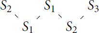
Note that in the above situation the Brauer tree of such a block is as below and the result follows easily from the structure of the only PIM belonging to the block.

Definition 3.2.

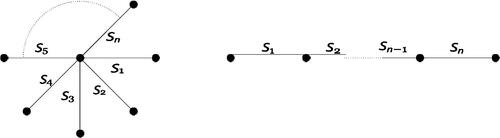
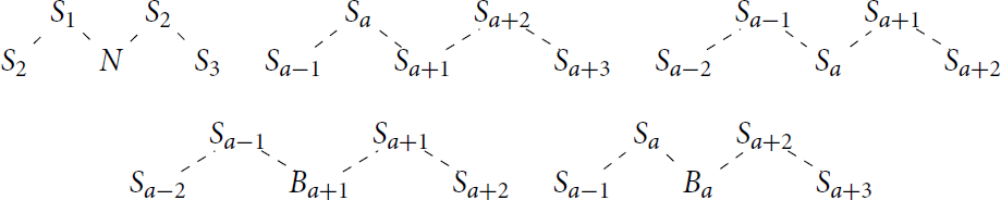
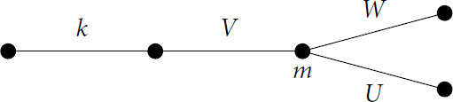
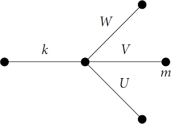
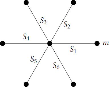
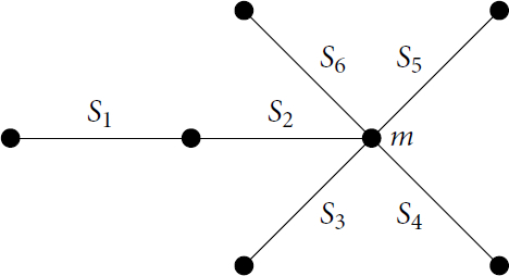
A star is a tree with n vertices, one of which has degree n – 1 and all others have degree 1 (alternatively, one may regard this as a complete bipartite graph $K_{1,n-1}$). If k is a field of characteristic p, B a p-block of a finite group and the Brauer tree of kB is a star then we may represent this as on the left in Figure 1. In such a case, the exceptional vertex (if it exists) is either the central vertex (as drawn) or any other vertex. We choose our notation so that if the exceptional vertex is an outer one, it is connected to the simple module S₁.

Fig. 1 A star and a line.

The following is immediate from the Brauer tree in question.

Proposition 3.3.

Suppose that B is a p-block of a finite group G whose Brauer tree is a star. If the exceptional vertex is the central vertex with exceptionality $m\ge 1$ then the projective cover of S_i has shape $\mathcal{P}(S_i)\sim [S_i|M_i\left|S_i\right|\cdots \left|M_i\right|S_i]$, where $M_i\sim [S_{i+1}|S_{i+2}|\cdots |S_{i+n-1}]$ with indices taken mod n. Otherwise the exceptional vertex is an outer vertex with exceptionality m > 1 and $\mathcal{P}(S_i)\sim [S_i|M_i|S_i]$ for all $i\ne 1$ and $\mathcal{P}(S_1)\sim [S_1|M_1\oplus N|S_1]$ where $N\sim [S_1|S_1|\cdots |S_1]$ is uniserial and contains S₁ as a composition factor with multiplicity m.

Definition 3.4.

A line (also called an open polygon) is a tree with two vertices of degree one and a Hamiltonian path between them (that is, a path including all vertices). If k is a field of characteristic p, B a p-block of a finite group and the Brauer tree of kB is a line then we may represent this as on the right in Figure 1. In such a case, the exceptional vertex (if it exists) is either an endpoint or an interior vertex. We choose our notation so that if the exceptional vertex is an outer one then it is connected to the simple module S₁ and otherwise it is connected to the simple modules S_a and $S_{a+1}$ with $a\ge \frac{n}{2}$.

Again the following is immediate from the Brauer tree.

Proposition 3.5.

Suppose that B is a p-block of a finite group G whose Brauer tree is a line. If the exceptional vertex is an outer vertex with exceptionality m > 1 then $\mathcal{P}(S_i)\sim [S_i|S_{i-1}\oplus S_{i+1}|S_i]$ for all $1<i<n,\mathcal{P}(S_n)\sim [S_n|S_{n-1}|S_n]$ and $\mathcal{P}(S_1)\sim [S_1|S_2\oplus N|S_1]$ where $N\sim [S_1|S_1|\dots |S_1]$ has S₁ as a composition factor with multiplicity m. Otherwise the exceptional vertex is inner with exceptionality $m\ge 1$ and $\mathcal{P}(S_i)\sim [S_i|[S_{i-1}\oplus S_{i+1}|S_i]$ for all $1<i<n$ not a or a + 1, $\mathcal{P}(S_1)\sim [S_1|S_2|S_1],\mathcal{P}(S_n)\sim [S_n|S_{n-1}|S_n]$. Finally, $\mathcal{P}(S_a)\sim [S_a|S_{a-1}\oplus B_a|S_a]$ and $\mathcal{P}(S_{a+1})\sim [S_{a+1}|B_{a+1}\oplus S_{a+2}|S_{a+1}]$ where $B_a\sim [S_{a+1}|S_a\left|S_{a+1}\right|\cdots |S_{a+1}]$ contains each of S_a and $S_{a+1}$ as composition factors with multiplicity m and $B_{a+1}$ is similar but with a and a + 1 swapped.

We close out this section by determining the Exts in the case where the Brauer tree is a star, the case where the Brauer tree is a line is significantly more complex and is the focus of Section 4. The following result can in fact be seen from [8, (5.5)] which computes the Heller translates of normalizers of p-groups (which are all stars with central exceptional vertex).

Proposition 3.6.

Suppose G is a finite group and B is a block of kG whose Brauer tree is a star with exceptional vertex of exceptionality $m\ge 1$ at its centre. Suppose that the irreducible kG-modules lying in B are $\{S_1,\dots ,S_n\}$. Then ${\text{Ext}}_G^{\mathcal{l}}(S_i,S_j)$ is 1-dimensional when $\mathcal{l}\equiv j-i$ or $j-i+1\hspace{1em}\mathrm{\text{mod}}2n$ and zero otherwise.

Proof.

Recall the structure of the PIMs in this case from Proposition 3.3. It is then easy to check that $\Omega S_i\sim [S_{i+1}|M_{i+1}|\cdots |M_{i+1}|S_i]\sim \text{rad}\mathcal{P}(S_{i+1})$, so ${\Omega }^2{S}_i\cong S_{i+1}$ and the result follows from Lemma 2.3. □

Proposition 3.7.

Suppose G is a finite group and B is a block of kG whose Brauer tree is a star with exceptional vertex of exceptionality $m>1$ an outer vertex. Suppose that the irreducible kG-modules lying in B are $\{S_1,\dots ,S_n\}$ with S₁ connected to the exceptional vertex. Then ${\text{Ext}}_G^{\mathcal{l}}(S_i,S_j)$ is 1-dimensional when $i=j=1$ or $\mathcal{l}\equiv j-i$ or $j-i-1\hspace{1em}\mathrm{\text{mod}}2n$ and zero otherwise.

Proof.

Recall again the structure of the PIMs from Proposition 3.3. If i is neither 1 nor n then ${\Omega }^2{S}_i\cong S_{i+1}$ as in Proposition 3.6. It is then easily calculated that $\Omega S_n\sim [S_1|M_1],{\Omega }^2{S}_n\sim [N|S_1]$ and ${\Omega }^3{S}_n\sim [M_1|S_1]$ so that ${\Omega }^4{S}_n\sim S_2$.

This gives us the dimensions of all but ${\text{Ext}}_G^{\mathcal{l}}(S_1,S_1)$. We claim that ${\text{Ext}}_G^{\mathcal{l}}(S_1,S_1)$ is 1-dimensional for all $\mathcal{l}$ (note this also follows from Theorem 0.5 in the recent preprint [2]). Suppose not, and in particular suppose that t > 0 is minimal such that ${\text{Ext}}_G^t(S_1,S_1)=0$. Using [12, Theorem 5.16] we see that any non-projective indecomposable module stemming from a path in the Brauer tree not containing the exceptional vertex must stem from a path as in [12, (5.2)] (that is, a path which does not go back on itself). In our case, such a path may contain only two edges and as such yields a uniserial module, so any non-projective indecomposable module M such that ${\text{Hom}}_G(M,S_1)=0$ is uniserial.

In particular, ${\Omega }^t{S}_1$ is a non-projective indecomposable module with ${\text{Hom}}_G({\Omega }^t{S}_1,S_1)=0$ and thus is a uniserial module. Hence ${\Omega }^t{S}_1$ is a quotient of some $\mathcal{P}(S_i)$ for $i\ne 1$, so ${\Omega }^t{S}_1\sim [S_i|S_{i+1}|\cdots |S_{i+j}]$ for j < n and indices taken mod n. Then we see that ${\Omega }^{t-1}{S}_1\sim [S_{i+j}|S_{i+j+1}|\cdots |S_{i-1}]\sim [S_1\left|S_2\right|\cdots |S_{i-1}]$ by the minimality of t. But then ${\Omega }^{t-2}{S}_1\sim [S_{i-1}|S_i|\cdots |S_n]$ and so ${\text{Ext}}_G^{t-2}(S_1,S_1)=0$, contradicting the minimality of t. □

4 Lines

For this section, suppose that B is a block of kG whose Brauer tree is a line with exceptional vertex of exceptionality m. If $m=1$, we are done by [5]. To deal with the case where m > 1, we adapt the notation from [2, 5]. We leave the definitions of ${}^i\mathrm{}{X}^j,{}^i\mathrm{}{X}_j,{}_i{X}^j$, and ${}_i{X}_j$ unchanged for i, $j\ge 1$ and each module is respectively defined to be the unique indecomposable module of the below described shape.

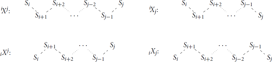
This means that the modules in the bottom “row” of the module ${}^i\mathrm{}{X}^j$ above are all submodules of ${}^I\mathrm{}{X}^j$ and those in the top “row” all lie in the quotient by the bottom “row” with the dashed lines representing non-split extensions. For example, taking a quotient of ${}^i\mathrm{}{X}^j$ by the unique submodule isomorphic to $S_{i+1}$ would yield a module $S_i{\oplus }^{i+2}\mathrm{}{X}^j$.

To allow for consistency with future notation, we also define ${}^i{Y}^j:{=}^i\mathrm{}{X}^j,{}^i{Y}_j:{=}^i\mathrm{}{X}_j,{}_i{Y}^j:{=}_i{X}^j$ and ${}_i{Y}_j:{=}_i{X}_j$.

Extending this, we also define ${}^{-i}\mathrm{}{X}^j,{}^{-i}{Y}^j$, ${}^i\mathrm{}{Z}^j$ and similar variants thereof. For positive integers i, j, when ${\text{Ext}}_G^1(S_1,S_1)\ne 0$ we define ${}^{-i}\mathrm{}{X}^j$ to be the unique indecomposable module of shape

Suppose that the exceptional vertex is an outer vertex and recall the definition of N from Proposition 3.5. We define ${}^{-i}{Y}^j$ to be the unique indecomposable module of shape

We also define ${}^{-i}\mathrm{}{X}^{-j}:{=}^j\mathrm{}{X}^i={:}^{-i}{Y}^{-j}$. Finally, suppose that the exceptional vertex is an inner vertex and recall that S_a and $S_{a+1}$ are incident to the exceptional vertex. Take $B_a\sim [S_{a+1}|S_a\left|S_{a+1}\right|\dots |S_{a+1}],B_{a+1}\sim [S_a|S_{a+1}\left|S_a\right|\dots |S_a]$ as in Proposition 3.5. We define ${}^i\mathrm{}{Z}^j$ for $i\equiv a\hspace{1em}\mathrm{\text{mod}}2$ to be the unique indecomposable module of shape

and for $i\equiv a+1\hspace{1em}\mathrm{\text{mod}}2$ it is instead defined to be the unique indecomposable module of the below shape.

The other variants ${}^{-i}{Y}_j,{}_{-i}{X}^j,{}_{-i}{Z}_j$, etc. are all defined identically except the endpoints change exactly as on page 4.

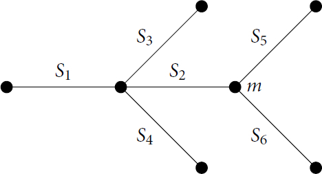
We will first consider the case where the Brauer tree of B is a line with the exceptional vertex an outer vertex. We may suppose that the Brauer tree and simple modules S_i are as below.

The dimensions of the $\text{Ext}$s in this case will follow from computing the Heller translate of various X, Y, and Z above. To reduce repetition, note that we may look only at the endpoints (as drawn) of these modules and their types (X, Y or Z). As such, we will state results for one endpoint and type at a time where possible. For example, $\Omega {(}^{i}W){\cong }^{i-1}W$ means both $\Omega {(}^i\mathrm{}{X}^j){\cong }^{i-1}\mathrm{}{X}^{j_1}$ and $\Omega {(}^i{Y}_j){\cong }^{i-1}{Y}_{j_2}$ for j₁, j₂ as given by the corresponding rules for X^j and Y_j . We now begin by stating some rules which cover most of the simpler cases.

Lemma 4.1.

Let $W\in \{X,Y,Z\}$. Define functions ${}_{*}\Omega ,{}^{*}\Omega$, ${\Omega }_{*},{\Omega }^{*}$ and $\Omega {\prime }_{\mathit{\text{ij}}}$ (for $i\ne -n,j\ne n$ and, if there is no exceptional vertex, $i\ne 1$) such that $$\Omega {(}_{i_l}^{i_u}{W}_{j_l}^{j_u}){\cong }_{{}_{*}\Omega (i_l)}^{{}^{*}\Omega (i_u)}{(\Omega {\prime }_{\mathit{\text{ij}}}W)}_{{\Omega }_{*}(j_l)}^{{\Omega }^{*}(j_u)}$$ where i is the value of whichever of i_u or i_l is defined, and similarly for j. Then we have the following:

1. if i < 0, ${\Omega }_{\mathit{\text{ij}}}^{\prime }X=Y$;

2. ${\Omega }_{\mathit{\text{ij}}}^{\prime }Y=X$;

3. if the exceptional vertex is an inner vertex and i < a or $j>a+1$ we have ${\Omega }_{\mathit{\text{ij}}}^{\prime }X=Z$, otherwise ${\Omega }_{\mathit{\text{ij}}}^{\prime }X=X$;

4. ${\Omega }_{\mathit{\text{ij}}}^{\prime }Z=X$;

5. if $i\ne \pm 1$, – n and $j\ne \pm 1$, n we have ${}_{*}\Omega (i)=i+1,{}^{*}\Omega (i)=i-1,{\Omega }_{*}(j)=j-1$ and ${\Omega }^{*}(j)=j+1$,

6. in all cases, $\Omega W^n\cong {({\Omega }_{\mathit{\text{in}}}^{\prime }(W))}_n$ and $\Omega {(}^{-n}W){\cong }_{-n}({\Omega }_{-\mathit{\text{nj}}}^{\prime }(W))$.

Proof.

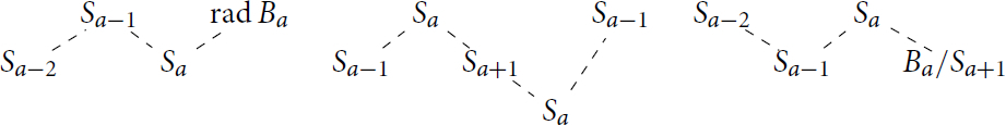
For this, we only consider the section of the modules in question made up of the composition factors which are “close to” the exceptional vertex in the Brauer graph as the rest is identical to the arguments used in [5, Lemma 2.1]. For i), note that for suitable i and j, X has a section ${}_{-3}{Y}_2$ of shape

with projective cover $$\begin{array}{c}{S}_2\\ S_3\oplus S_1\\ S_2\end{array}\oplus \begin{array}{c}{S}_1\\ N\oplus S_2\\ S_1\end{array}.$$

It is then easy to see here that the kernel of such a cover must have shape $[S_1|S_2\oplus N]$ as in Y. When the above section of X is not the whole module, one may patch this together as in [14, Lemma 3.18] to obtain i), and when i or j are too small only minor modifications are needed. Parts ii)–iv) follow from an identical argument examining the sections

of Y, X, X, Z, and Z, respectively (note the duplicate Xs and Zs because this case depends on whether $i\equiv a\hspace{1em}\mathrm{\text{mod}}2$). Finally, v) and vi) are obvious due to the structure of the projective covers of simple modules not incident to the exceptional vertex. □

Lemma 4.2.

Suppose that B is a p-block of a finite group G whose Brauer tree is a line with exceptional vertex an outer vertex (without loss of generality, S₁ is incident to the exceptional vertex). Then we have the following isomorphisms.

1. $\Omega {(}^1\mathrm{}X){\cong }^{-1}Y$

2. $\Omega {(}^{-1}Y){\cong }^{-2}X$

3. $\Omega {(}_{-1}X){\cong }_{1}Y$

4. $\Omega Y_1\cong Y_{-1}{\cong }_{1}X$

Proof.

As with the previous cases, we focus only on a small section of the module in question. To see i) and ii), note that the Heller translate of a section of shape $[S_1\oplus S_3|S_2]$ of ${}^1\mathrm{}X$ has shape $[S_1\oplus S_2|N\oplus S_3]$, yielding i), and the Heller translate of the section just obtained has shape

For iii), the Heller translate of a section of shape $[S_1|S_1\oplus S_2]$ of ${}_{-1}X$ has shape $[S_2\oplus S_4|N\oplus S_3]$ as in ${}_{1}Y$ and for iv) note that the Heller translate of $[S_1|S_2\oplus N]$ is $[S_2|S_1]$. □

Proposition 4.3.

Suppose G is a finite group and B is a block of kG whose Brauer tree is a line with exceptional vertex of exceptionality $m>1$ an outer vertex as described in Definition 3.4. Then $\mathrm{\text{dim}}{\text{Ext}}_G^{\mathcal{l}}(S_i,S_j)$ is nonzero (thus 1-dimensional) for $j\ne 1$ precisely when either of the following hold (where values of $\mathcal{l}$ are taken modulo 2n) $$\{\begin{array}{cc}\mathcal{l}\equiv |i-j|\hspace{1em}\mathrm{\text{mod}}2\hfill & \text{if }|i-j|\le \mathcal{l}\le 2n-i-j\hfill \\ \mathcal{l}\equiv |i-j|+1\hspace{1em}\mathrm{\text{mod}}2\hfill & \text{if }i+j-1\le \mathcal{l}\le 2n-|i-j|-1\hfill \end{array}$$

Further, ${\text{Ext}}_G^{\mathcal{l}}(S_i,S_1)$ is nonzero precisely when $i-1\le \mathcal{l}\le 2n-i$.

Proof.

This follows from the fact that we may regard S_i as ${}^i\mathrm{}{X}^i$ and then repeatedly use Lemmas 4.1 and 4.2. We illustrate below the case where $i<\frac{n}{2}$, j > i and $i\equiv j\hspace{1em}\mathrm{\text{mod}}2$.

For $\mathcal{l}<j-i$, S_j clearly does not lie in the head of ${\Omega }^{\mathcal{l}}{S}_i={\Omega }^{\mathcal{l}}{}^i\mathrm{}{X}^i$ but ${\Omega }^{j-i}{S}_i$ has ${}^i\mathrm{}{X}^j$ as a quotient. Then S_j will remain the head of every second Heller translate of this module until we reach ${\Omega }^{2n-i-j}{S}_i$ since ${\Omega }^{n-i}{S}_i$ has quotient ${}^i\mathrm{}{X}^n$ and ${\Omega }^{n-j+1}(X^n)=Y_j$ which does not have S_j in its head; this gives nonzero $\text{Ext}$s for $j-i\le \mathcal{l}\le 2n-i-j$ for $\mathcal{l}$ even. For the other range, note that ${\Omega }^i{S}_i{\cong }^{-1}\mathrm{}{Y}^{2i+1}$ and so ${\Omega }^{i-1+j}{S}_i$ has quotient ${}^{-j}\mathrm{}{Y}^1$, giving ${\text{Ext}}_G^{i+j-1}(S_i,S_j)\ne 0$ but no earlier odd-indexed nonzero $\text{Ext}$. Again, we see that S_j remains in the head of every second Heller translate of this module until we reach ${\Omega }^{2n-|i-j|-1}$ as ${\Omega }^{n+i-1}$ has quotient ${}^{-n}\mathrm{}{X}^{-i}{\cong }^i\mathrm{}{X}^n$ and as before ${\Omega }^{n-j+1}(X^n)$ does not have S_j in its head, so nor does ${\Omega }^{2n+i-j-1}{S}_i$, yielding the second range of values of $\mathcal{l}$ in the statement.

Note that if j < i then ${\Omega }^{2n-i+1}{S}_i$ has quotient ${}_{-i}{Y}_{-1}{\cong }_1{Y}_i$ and ${\Omega }^{j-1}{(}_{1}X){\cong }_{j}X$ which does not have S_j in its head, giving instead a range of $i+j-1\le \mathcal{l}\le 2n+j-i-1=2n+|i-j|-1$. All remaining cases require only minor modifications to the above. □

We now consider the other case, where the Brauer tree of B is a line but the exceptional vertex is an inner vertex. Suppose that the exceptional vertex connects the simple modules S_a and $S_{a+1}$, then we may assume the Brauer tree of B is as below.

In this case, for $i\ne 1$, a, a + 1 or n, we have that $\mathcal{P}(S_i)\sim [S_i|S_{i-1}\oplus S_{i+1}|S_i]$ as above and $\mathcal{P}(S_1)\sim [S_1|S_2|S_1],\mathcal{P}(S_n)\sim [S_n|S_{n-1}|S_n]$, leaving us with $\mathcal{P}(S_a)\sim [S_a|S_{a-1}\oplus B_a|S_a]$ and $\mathcal{P}(S_{a+1})\sim [S_{a+1}|B_{a+1}\oplus S_{a+2}|S_{a+1}]$ where $B_a\sim [S_{a+1}|S_a\left|S_{a+1}\right|\cdots |S_{a+1}]$ and $B_{a+1}\sim [S_a|S_{a+1}\left|S_a\right|\cdots |S_a]$.

Lemma 4.4.

Let B be a p-block of a finite group G whose Brauer tree is a line with exceptional vertex an inner vertex as described in Definition 3.4. We have $\Omega {(}^1\mathrm{}Z){\cong }_{1}X$ and $\Omega {(}^1\mathrm{}X){\cong }_{1}Z$ if S_a or $S_{a+1}$ lie in the head of ${}^1\mathrm{}X$ and ${}_{1}X$ otherwise. Further, ${\Omega }_a{Z}_a{\cong }^{a-1}\mathrm{}{X}^{a+1}$ and ${\Omega }_{a+1}{Z}_{a+1}{\cong }^a\mathrm{}{X}^{a+2}$.

Proof.

The first two statements are similar to Lemma 4.1 iii), iv), thus left as an exercise, and the final statements follow easily from the fact that ${}_a{Z}_a\cong B_{a+1}$ and ${}_{a+1}{Z}_{a+1}\cong B_a$. □

Proposition 4.5.

Suppose G is a finite group and B is a block of kG whose Brauer tree is a line with exceptional vertex of exceptionality $m>1$ an inner vertex as described in Definition 3.4. Then $\mathrm{\text{dim}}{\text{Ext}}_G^{\mathcal{l}}(S_i,S_j)$ for $i\ne a$ is nonzero (thus 1-dimensional) precisely when either of the following hold (where values of $\mathcal{l}$ are taken modulo 2n) $$\{\begin{array}{cc}\mathcal{l}\equiv |i-j|\hspace{1em}\mathrm{\text{mod}}2\hfill & \text{if }|i-j|\le \mathcal{l}\le \mathrm{\text{min}}\{i+j-2,2n-i-j\}\hfill \\ \mathcal{l}\equiv |i-j|+1\hspace{1em}\mathrm{\text{mod}}2\hfill & \text{if }|n-i-j+1|+n\le \mathcal{l}\le 2n+|i-j|-1\hfill \end{array}$$

If $a=\frac{n}{2}$ then ${\text{Ext}}_G^{\mathcal{l}}(S_a,S_j)$ follows the same rules as above, otherwise $a>\frac{n}{2}$ and we have ${\text{Ext}}_G^{\mathcal{l}}(S_a,S_j)$ nonzero precisely when any of the below conditions hold. $$\{\begin{array}{cc}\mathcal{l}\equiv |a-j|\hspace{1em}\mathrm{\text{mod}}2\hfill & \text{if }|a-j|\le \mathcal{l}\le \mathrm{\text{min}}\{a+j-2,2n-a-j\}\hfill \\ a\ge \mathcal{l}\equiv |a-j|+1\hspace{1em}\mathrm{\text{mod}}2\hfill & \text{if }2n-a-j+1\le \mathcal{l}\le 2n+|a-j|-1\hfill \\ a<\mathcal{l}\equiv |a-j|+1\hspace{1em}\mathrm{\text{mod}}2\hfill & \text{if }|n-a-j+1|+n\le \mathcal{l}\le 2n+|a-j|-1\hfill \end{array}$$

Proof.

As above, we may regard S_i as ${}^i\mathrm{}{X}^i$ and repeatedly use Lemmas 4.1 and 4.4. For $i\ne a$ proceed in a manner identical to Proposition 4.3 to obtain the result. We will illustrate here the case where $j>i=a>\frac{n}{2}$ as this is slightly more complicated but still encompasses the arguments required for all other cases, with the case $i=a+1$ being similar again so left as an exercise.

Regard S_a as ${}^a\mathrm{}{X}^a$ and note that, as usual, S_j does not lie in the head of ${\Omega }^{\mathcal{l}}{S}_a$ for $\mathcal{l}<j-a$ but is in the head of ${\Omega }^{j-a}{S}_a$ as well as every second Heller translate of this module until ${\Omega }^{2n-a-j}{S}_a\cong W_j$ for $W\in \{X,Z\}$ dependent on whether $j\equiv a\hspace{1em}\mathrm{\text{mod}}2$. Continue in this way until we reach ${\Omega }^{2(n-a)}{S}_a\cong Y_{a+1}$ where we can no longer rely on Lemma 4.1. Take a section ${}_{a-3}{Y}_{a+1}$ of the aforementioned module and note that this has Heller translates

with the third module above having Heller translate ${}^{a-3}\mathrm{}{X}^{a+1}$. Note also that if the second module above was attached to a module $[S_{a-3}|S_{a-2}]$ on the left as drawn above, the third Heller translate would instead be

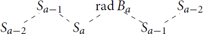
From this we can see that the Heller translates of ${\Omega }^{2(n-a)}{S}_a$ will alternate between modules with sections of the second and fourth shapes above until reaching ${\Omega }^{2a-1}{S}_a$ with section of the third shape (and no $S_{a+1}$ in the socle), yielding ${\Omega }^{2a}{S}_i\cong X^{a+1}$, whereupon the Heller translates resume alternating between X and Z until we reach ${\Omega }^{2n}{S}_i\cong S_i$. Keeping track of the heads of these modules along the way yields the result. □

This leaves only the case where there is no exceptional vertex, which has already been done in [5, Proposition 2.2] though may also be obtained by mimicking the proof of Proposition 4.3 with ${\Omega }^1\mathrm{}X{=}_{1}X$ rather than ${}^{-1}Y$.

Proposition 4.6.

Suppose G is a finite group and B is a block of kG whose Brauer tree is a line with no exceptional vertex as described in Definition 3.4. Then $\mathrm{\text{dim}}{\text{Ext}}_G^{\mathcal{l}}(S_i,S_j)$ is nonzero (thus 1-dimensional) precisely when either of the following hold (where values of $\mathcal{l}$ are taken modulo 2n) $$\{\begin{array}{cc}\mathcal{l}\equiv |i-j|\hspace{1em}\mathrm{\text{mod}}2\hfill & \text{if }|i-j|\le \mathcal{l}\le 2n-i-j\hfill \\ \mathcal{l}\equiv |i-j|+1\hspace{1em}\mathrm{\text{mod}}2\hfill & \text{if }i+j-1\le \mathcal{l}\le 2n-|i-j|-1\hfill \end{array}$$

5 ${\text{PSU}}_3(q)$

When the Sylow r-subgroups of $G:={\text{PSU}}_3(q)$ are cyclic, the Brauer trees of all r-blocks of G are lines or a star with three points [7]. In any such case, we are done by Propositions 4.5, 3.6, and 3.1. Otherwise, the Sylow r-subgroups of G are not cyclic, and when r > 2 divides q + 1 or r = 2 and $q\equiv 3\hspace{1em}\mathrm{\text{mod}}4$ the representation type of kG is wild and the structure of the PIMs is not known. As such, determining the dimensions of cohomology or $\text{Ext}$ groups in this case is outside the scope of this work.

6 Extensions and cohomology in $\text{Sz}(q)$

We next deal with the Suzuki groups $G:=\text{Sz}(q)$ (also denoted ${}^2{B}_2(q)$) for $q=2^{2n+1}$ where $n\ge 1$ (note here we mean that for n > 0, G is a finite simple group and for a = 0 we have $G\cong C_5⋊C_4$), since the Sylow r-subgroups of these groups in non-defining characteristics are cyclic and so methods used before all apply. In particular, the Brauer trees are known due to Burkhardt [3] for the Suzuki groups for all such cases and so we know the structure of the projective modules in these cases very well.

We will not require any structural information about $\text{Sz}(q)$ as the results are determined completely by the structure of the projective modules (thus the Brauer trees), but the curious reader should consult [4, Chapters 13 and 14] for more. These groups have order $|\text{Sz}(q)|=q^2(q-1)(q^2+1)$ which factors as $q^2(q-1)(q-s+1)(q+s+1)$, where $s^2=2q$, and so the study of the cross characteristic representation theory of these groups splits naturally into the three cases $r|q-1,r|q-s+1$ and $r|q+s+1$. For convenience, we reproduce the character table of $\text{Sz}(q)$ from [3] and label the complex characters accordingly.

Let x, y, and z be elements of $\text{Sz}(q)$ of orders q – 1, $q+s+1$ and $q-s+1$, respectively, and let f and t be elements of respective orders 4 and 2. Powers of these elements give a set of conjugacy class representatives for G. Now, let ω, η, and ζ be primitive $(q-1)$ th, $(q-s+1)$ th, and $(q+s+1)$th complex roots of unity, respectively, and let ${\epsilon }_d:={\zeta }^d+{\zeta }^{-d}+{\zeta }^{\mathit{\text{qd}}}+{\zeta }^{-\mathit{\text{qd}}}$ and ${\delta }_e:={\eta }^e+{\eta }^{-e}+{\eta }^{\mathit{\text{qe}}}+{\eta }^{-\mathit{\text{qe}}}$. Finally, let a, $u\le \frac{1}{2}(q-2)$; b, $l\le \frac{1}{4}(q+s)$; c, $v\le \frac{1}{4}(q-s)$ and of course $i=\sqrt{-1}$, where a, b, c, l, u and v are all positive integers. Then the ordinary character table of G is as below.

We begin by considering the case where $r|q-1$. In this case, the modules with characters Γ_i , θ_i and Λ_i lie in blocks of defect zero and thus are projective. The principal r-block of G consists of two modules, k and V, where k is the trivial module as usual and $\mathrm{\text{dim}}V=q^2$. The remaining modules lie alone in blocks of maximal defect. From [3, 423], the Brauer tree of the principal block is a line with two edges whose central vertex is exceptional with exceptionality $m=\frac{r^x-1}{2}$, where r^x is the r-part of q – 1. This is the same Brauer tree as in [14, Proposition 3.6], and so we already know the answer for the principal block. Alternatively, we may also use Proposition 4.5 to obtain the following result with the final statement following from Proposition 3.1.

Proposition 6.1.

Let $G=\text{Sz}(q)$ and suppose that r is an odd prime dividing $q-1$. Let V be the nontrivial irreducible module lying in the principal block. Then $V=V^{*}$, thus ${\mathrm{H}}^n(G,V)\cong {\text{Ext}}_G^n(V,k)$, for all n and $${\mathrm{H}}^n(G,k)\cong {\text{Ext}}_G^n(V,V)\cong \{\begin{array}{cc}0\hfill & n\equiv 1,2\hspace{1em}\mathrm{\text{mod}}4,\hfill \\ k\hfill & n\equiv 0,3\hspace{1em}\mathrm{\text{mod}}4,\hfill \end{array}\hspace{1em}{\mathrm{H}}^n(G,V)\cong \{\begin{array}{cc}k\hfill & n\equiv 1,2\hspace{1em}\mathrm{\text{mod}}4,\hfill \\ 0\hfill & n\equiv 0,3\hspace{1em}\mathrm{\text{mod}}4.\hfill \end{array}$$

Any non-projective irreducible module W lying outside the principal block (so W has character Ω_i for some i) is such that ${\text{Ext}}_G^n(W,W)\cong k$ for all n.

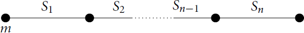
We now consider the case where $r|q-s+1$. In this case, the modules with characters Ω_i and θ_i are projective and the principal r-block of G contains 4 modules k, U, V, and W. Here, V has dimension $q^2-1$ and $U\cong W^{*}$ each have dimension $\frac{s}{2}(q-1)$. The remaining modules lie alone in blocks of maximal defect. From [3, 424], the Brauer tree for the principal r-block of G is as below with exceptionality $m=\frac{r^x-1}{4}$ where r^x is the r-part of $q-s+1$.

From this, we see that the projective modules in the principal block are as follows: $\mathcal{P}(k)\sim [k|V|k],\mathcal{P}(U)\sim [U|W\left|V\right|U|\cdots |V|U],\mathcal{P}(W)\sim [W|V\left|U\right|W|\cdots |V\left|U\right|W]$ and $\mathcal{H}\mathcal{P}(V):=\text{rad}(\mathcal{P}(V))/\text{soc}(\mathcal{P}(V))\cong k\oplus Y_V$ where $Y_V\sim [U|W\left|V\right|\cdots \left|U\right|W]$.

Proposition 6.2.

Let $G=\text{Sz}(q)$ and suppose that r is an odd prime dividing $q-s+1$ for $s=\sqrt{2q}$. Then the value of ${\text{Ext}}_G^n(M,N)$, for irreducible M, N in the principal r-block of G, is nonzero for precisely the values of n modulo 8 given in the below table. Here, the entry in row M, column N gives the values of n modulo 8 for which ${\text{Ext}}_G^n(M,N)\cong k$. $$\begin{array}{ccccc}& k& U& V& W\\ k& 0,7& 2,3& 1,6& 4,5\\ U& 4,5& 0,7& 3,6& 1,2\\ V& 1,6& 1,4& 0,2,5,7& 3,6\\ W& 2,3& 5,6& 1,4& 0,7\end{array}$$

All non-projective irreducible modules M outside of the principal block (these are the modules with characters Λ_i) are such that ${\text{Ext}}_G^n(M,M)\cong k$ for all n.

The latter statement is a direct consequence of Proposition 3.1. The remainder of the proof of Proposition 6.2 is given as the combination of the following two propositions.

Proposition 6.3.

The dimensions of ${\text{Ext}}_G^n(M,N)$ are as in the table in Proposition 6.2 for $(M,N)\in {\{k,U,V,W\}}^2\setminus \{(V,V)\}$.

Proof.

Throughout, the reader should refer to the structure of the projective modules given before Proposition 6.2. We proceed in the usual way, examining the structure of ${\Omega }^{n}k$. Let Y_U and Y_W denote $\mathcal{H}(\mathcal{P}(U))$ and $\mathcal{H}(\mathcal{P}(W))$, respectively, and note that $\text{head}{Y}_U\cong W,\text{ head}{Y}_V\cong U$ and $\text{head}{Y}_W\cong V$. Where $\text{head}{\Omega }^{n}V$ is simple, the structure of ${\Omega }^{n+1}V$ may be immediately read off from the shape of $\mathcal{P}({\Omega }^{n}V)$.

First, note that $\Omega k$ has shape $[V|k]$ and thus ${\Omega }^{2}k$ must have shape $[Y_V|V]$. Then ${\Omega }^{3}k\cong U$ and so ${\Omega }^{4}k\cong \Omega U$ has shape $[Y_U|U]$. This then immediately gives ${\Omega }^{5}k\cong W$, leading to ${\Omega }^{6}k\cong \Omega W$ with shape $[Y_W|W]$. Finally, this gives ${\Omega }^{7}k$ of shape $[k|V]$ and thus ${\Omega }^{8}k\cong k$, so as in the previous case we see that k, U, and W are periodic of period 8. By examining the heads of these modules (and using the fact that ${\text{Ext}}_G^n(M,N)\cong {\text{Ext}}_G^n(N^{*},M^{*})$) we obtain the desired result. □

Proposition 6.4.

The dimensions of ${\text{Ext}}_G^n(V,V)$ are as in the table in Proposition 6.2. In particular, ${\text{Ext}}_G^n(V,V)\cong k$ precisely when $n\equiv 0$, 2, 5 or $7\hspace{1em}\mathrm{\text{mod}}8$.

Proof.

As with the previous case, we examine the structure of ${\Omega }^{n}V$ while referring continually to the structure of the projective modules given before Proposition 6.2. We first provide the shapes of ${\Omega }^{n}V$ for $n=1,$ …, 8. $$\begin{array}{cccc}\Omega V\sim \begin{array}{c}k\oplus Y_V\\ V\end{array}\hfill & {\Omega }^{2}V\sim \begin{array}{c}V\\ k\oplus U\end{array}\hfill & {\Omega }^{3}V\sim \hspace{1em}{Y}_U\hfill & {\Omega }^{4}V\sim \begin{array}{c}U\\ W\end{array}\hfill \\ {\Omega }^{5}V\sim \hspace{1em}{Y}_W\hfill & {\Omega }^{6}V\sim \begin{array}{c}k\oplus W\\ V\end{array}\hfill & {\Omega }^{7}V\sim \begin{array}{c}{Y}_W\\ k\oplus W\end{array}\hfill & {\Omega }^{8}V\cong \hspace{1em}V\hfill \end{array}$$

The cases where ${\Omega }^{n-1}V$ has a simple head may be read off directly from the structure of its projective cover.

For ${\Omega }^{2}V$, note that the V in $\text{soc}\Omega V$ must come from a diagonal submodule of $\mathcal{H}\mathcal{L}\oplus \text{soc}{Y}_U$ in $\mathcal{L}\oplus \mathcal{P}(U)$. Similarly, for ${\Omega }^{7}V$, the V in $\text{soc}{\Omega }^{6}V$ must come from a diagonal submodule of $\mathcal{H}\mathcal{L}\oplus \text{head}{Y}_W$ in $\mathcal{L}\oplus \mathcal{P}(W)$. The result then follows by examining the heads of the above modules. □

Finally, we consider the case where $r|q+s+1$. In this case, the modules with characters Ω_i and Λ_i are projective and the principal r-block of G contains 4 simple modules: k, U, V and W where $U^{*}\cong W,\mathrm{\text{dim}}U=\mathrm{\text{dim}}W=\frac{s}{2}(q-1)$ and $\mathrm{\text{dim}}V=(q-1)(q-s+1)$. The remaining modules lie alone in blocks of maximal defect as before. From [3, 423], the principal block has the below Brauer tree with exceptionality $m=\frac{r^x-1}{4}$ where r^x is the r-part of $q+s+1$. Note that the case q = 2 is not covered in [3] but one may verify directly that the Brauer tree in this case is still as below with m = 1.

This Brauer tree is a star, so the below result then follows from Propositions 3.7, 3.1 (and Propositions 3.6 when $m=1$).

Proposition 6.5.

Let $G=\text{Sz}(q)$ and suppose that r is an odd prime dividing $q+s+1$ for $s=\sqrt{2q}$. Then, provided $m\ne 1$ (i.e. the r-part of $q+s+1$ is not 5) the value of ${\text{Ext}}_G^n(M,N)$, for irreducible M, N in the principal r-block of G, is nonzero for precisely the values of n modulo 8 given in the below table. Here, the entry in row M, column N gives the values of n modulo 8 for which ${\text{Ext}}_G^n(M,N)\cong k$. $$\begin{array}{ccccc}& k& U& V& W\\ k& 0,7& 1,2& 3,4& 5,6\\ U& 5,6& 0,7& 1,2& 3,4\\ V& 3,4& 5,6& \text{all}& 1,2\\ W& 1,2& 3,4& 5,6& 0,7\end{array}$$

When the r-part of $q+s+1$ is 5, we instead have ${\text{Ext}}_G^n(V,V)\cong k$ for $n\equiv 3,4\hspace{1em}\mathrm{\text{mod}}8$ and zero otherwise. Further, all non-projective irreducible kG-modules M outside the principal block (so M has character Θ_i for ${(q+s+1)}_{r\prime }\nmid i$) are such that ${\text{Ext}}_G^n(M,M)\cong k$ for all n.

7 Extensions and cohomology in ${}^2{G}_2(q)$

Finally, we deal with the Ree groups $G:{=}^2{G}_2(q)$ for $q=3^{2a+1}$ and $a\ge 0$ (note here we mean that for a > 0, G is a finite simple group and for a = 0 we have $G\cong \mathrm{P}\Gamma {\text{ L}}_2(8)$). Provided r > 3, all of the Sylow r-subgroups of G are cyclic and the Brauer trees for these cases may be found in [11, Section 4.1]. Note that the Sylow 2-subgroups of G are elementary abelian of order eight, and so the representation type in this case is wild and we do not consider this case here.

As in the case of the Suzuki groups, we will not require any structural information about G in this case as the results are dependent solely upon the Brauer trees of the blocks involved. These groups have order $\left|G\right|=q^3(q-1)(q^3+1)$ which factors as $q^3(q-1)(q+1)(q+s+1)(q-s-1)$ where $s=\sqrt{3q}$. As such, the study of the cross-characteristic representation theory of these groups splits naturally into the cases where r divides $q\pm 1$ or $q\pm s+1$ (noting that since r > 3 it may divide at most one such factor).

We first consider the case where $r|q-1$ (and so a > 0). From [11, Theorem 4.1], the blocks of maximal defect in this case have at most two irreducible kG-modules, and the Brauer trees of the two blocks with more than one irreducible module are lines with exceptional vertex in the middle.

Proposition 7.1.

Let $G{=}^2{G}_2(q)$ and suppose that r is an odd prime divisor of $q-1$. Then the only two blocks with more than one irreducible module contain only two, S₁ and S₂, such that, for $i\ne j$, $${\text{Ext}}_G^n(S_i,S_i)\cong \{\begin{array}{cc}0\hfill & n\equiv 1,2\hspace{1em}\mathrm{\text{mod}}4,\hfill \\ k\hfill & n\equiv 0,3\hspace{1em}\mathrm{\text{mod}}4,\hfill \end{array}\mathrm{\hspace{1em}}\mathrm{\hspace{1em}}{\text{Ext}}_G^n(S_i,S_j)\cong \{\begin{array}{cc}0\hfill & n\equiv 0,3\hspace{1em}\mathrm{\text{mod}}4,\hfill \\ k\hfill & n\equiv 1,2\hspace{1em}\mathrm{\text{mod}}4.\hfill \end{array}$$

All other non-projective irreducible modules S lie alone in their blocks and so ${\text{Ext}}_G^n(S,S)\cong k$ for all $n\ge 0$.

Proof.

The Brauer trees in this case are given in [11, Theorem 4.1]. The $\text{Ext}$s for blocks with these trees were previously worked out in [14, Proposition 3.6], but this also follows from Proposition 4.5. For all modules lying in blocks alone, we use Proposition 3.1. □

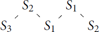
Next we suppose $2<r|q+1$ (and so a > 0). From [11, Theorem 4.2], the principal block has the below Brauer tree and there is one other block of maximal defect containing two irreducible kG-modules with Brauer tree a line with exceptional vertex on the outside.

In this case, the projective covers of all irreducible modules bar S₂ are uniserial. The heart of $\mathcal{P}(S_2)$ is of shape $[S_4|S_1|S_3]\oplus Y_2$ where $Y_2\sim [S_5|S_6\left|S_2\right|\cdots |S_6]$ and we denote the hearts of $\mathcal{P}(S_5)$ and $\mathcal{P}(S_6)$ by Y₅ and Y₆, respectively, where $Y_5\sim [S_6|S_2\left|S_5\right|\cdots |S_2]$ and $Y_6\sim [S_2|S_5\left|S_6\right|\cdots |S_5]$.

Proposition 7.2.

Let $G{=}^2{G}_2(q)$ and suppose that r is an odd prime divisor of q + 1. Then the $\text{Ext}$s for the principal block may be found in the below table, where the entries in row S_i, column S_j give those values of n mod 12 for which $\mathrm{\text{dim}}\text{Ext}(S_i,S_j)=1$. For all other values of n mod 12, this $\text{Ext}$ is zero. In this case, S₁ is the trivial module. $$\begin{array}{ccccccc}& S_1& S_2& S_3& S_4& S_5& S_6\\ S_1& 0,11& 3,8& 9,10& 1,2& 6,7& 4,5\\ S_2& 3,8& 0,2,4,5,6,7,9,11& 1,6& 5,10& 3,10& 1,8\\ S_3& 1,2& 5,10& 0,11& 3,4& 4,5& 6,7\\ S_4& 9,10& 1,6& 7,8& 0,11& 4,5& 2,3\\ S_5& 4,5& 1,8& 2,3& 6,7& 0,11& 9,10\\ S_6& 6,7& 3,10& 4,5& 8,9& 1,2& 0,11\end{array}$$

There is only one other block containing more than one irreducible module, which contains only two irreducible modules T₁, T₂, such that ${\text{Ext}}_G^n(T_2,T_2)\cong k$ for all n, and, for $i\ne j$, $${\text{Ext}}_G^n(T_1,T_1)\cong \{\begin{array}{cc}0\hfill & n\equiv 1,2\hspace{1em}\mathrm{\text{mod}}4,\hfill \\ k\hfill & n\equiv 0,3\hspace{1em}\mathrm{\text{mod}}4,\hfill \end{array}\mathrm{\hspace{1em}}\mathrm{\hspace{1em}}{\text{Ext}}_G^n(T_i,T_j)\cong \{\begin{array}{cc}0\hfill & n\equiv 0,3\hspace{1em}\mathrm{\text{mod}}4,\hfill \\ k\hfill & n\equiv 1,2\hspace{1em}\mathrm{\text{mod}}4.\hfill \end{array}$$

Finally, all other non-projective irreducible modules S lie alone in their blocks and so ${\text{Ext}}_G^n(S,S)\cong k$ for all $n\ge 0$.

Proof.

For the non-principal blocks with only one irreducible module, either this irreducible module is projective or we are done by Proposition 3.1. For the non-principal block with two irreducible modules, this was done in [14, Proposition 3.5] but also follows from Proposition 4.3. The bulk of the work in this case is used to determine the $\text{Ext}$s for the principal block, which we do now. Since all modules involved are uniserial, it is easy to calculate ${\Omega }^n{S}_1$ for $1\le n\le 12$ and observe the following. $$\begin{array}{cccccc}\Omega S_1\sim \begin{array}{c}{S}_4\\ S_2\\ S_3\\ S_1\end{array}\hfill & {\Omega }^2{S}_1\sim S_4\hfill & {\Omega }^3{S}_1\sim \begin{array}{c}{S}_2\\ S_3\\ S_1\\ S_4\end{array}\hfill & {\Omega }^4{S}_1\sim \begin{array}{c}{Y}_2\\ S_2\end{array}\hfill & {\Omega }^5{S}_1\sim S_6\hfill & {\Omega }^6{S}_1\sim \begin{array}{c}{Y}_6\\ S_6\end{array}\hfill \\ {\Omega }^7{S}_1\sim S_5\hfill & {\Omega }^8{S}_1\sim \begin{array}{c}{Y}_5\\ S_5\end{array}\hfill & {\Omega }^9{S}_1\sim \begin{array}{c}{S}_3\\ S_1\\ S_4\\ S_2\end{array}\hfill & {\Omega }^{10}{S}_1\sim S_3\hfill & {\Omega }^{11}{S}_1\sim \begin{array}{c}{S}_1\\ S_4\\ S_2\\ S_3\end{array}\hfill & {\Omega }^{12}{S}_1\sim S_1\hfill \end{array}$$

Examining the above fills all rows of the table bar the second, for which we need to also calculate ${\Omega }^n{S}_2$ for $1\le n\le 12$. This is somewhat more involved since the modules which appear are not all uniserial. The first few are still straightforward: $$\begin{array}{ccc}\Omega S_2\sim \begin{array}{c}\begin{array}{c}{S}_3\\ S_1\\ S_4\end{array}\oplus Y_2\\ S_2\end{array}\hfill & {\Omega }^2{S}_2\sim \begin{array}{c}{S}_2\\ S_3\oplus S_6\end{array}\hfill & {\Omega }^3{S}_2\sim \begin{array}{c}\begin{array}{c}{S}_1\\ S_4\end{array}\oplus \text{rad}{Y}_2\\ S_2\end{array}\hfill \\ {\Omega }^4{S}_2\sim \begin{array}{c}{S}_2\\ \begin{array}{c}{S}_3\\ S_1\end{array}\oplus \begin{array}{c}{S}_6\\ S_5\end{array}\end{array}\hfill & {\Omega }^5{S}_2\sim \begin{array}{c}{S}_4\oplus {\text{rad}}^2{Y}_2\\ S_2\end{array}\hfill & \hfill \end{array}$$

To compute ${\Omega }^6{S}_2$, take the submodule of $\mathcal{P}(S_4)\oplus \mathcal{P}(S_2)$ whose quotient is $S_4\oplus {\text{rad}}^2{Y}_2$. Then ${\Omega }^6{S}_2$ is the preimage in this submodule of a diagonal submodule of its head, which is of the below shape.

The remaining Heller translates are then again relatively straightforward. $$\begin{array}{ccc}{\Omega }^7{S}_2\sim \begin{array}{c}{S}_2{S}_2\\ \begin{array}{c}{\text{rad}}^3{Y}_2\\ S_2\end{array}\oplus S_3\end{array}\hfill & {\Omega }^8{S}_2\sim \begin{array}{c}\begin{array}{c}{S}_1\\ S_4\end{array}\oplus \begin{array}{c}{S}_6\\ S_5\end{array}\\ S_2\end{array}\hfill & {\Omega }^9{S}_2\sim \begin{array}{c}{S}_2\\ \begin{array}{c}{S}_3\\ S_1\end{array}\oplus \begin{array}{c}{\text{rad}}^2{Y}_6\\ S_6\end{array}\end{array}\hfill \\ {\Omega }^{10}{S}_2\sim \begin{array}{c}{S}_4\oplus S_5\\ S_2\end{array}\hfill & {\Omega }^{11}{S}_2\sim \begin{array}{c}{S}_2\\ \begin{array}{c}{S}_3\\ S_1\\ S_4\end{array}\oplus \begin{array}{c}\text{rad}{Y}_5\\ S_5\end{array}\end{array}\hfill & {\Omega }^{12}{S}_2\cong S_2\hfill \end{array}$$

The result then follows from examining the heads of the given modules. □

We next suppose that $2<r|q+s+1$. Then from [11, Theorem 4.3], the only block containing more than one irreducible kG-module is the principal block which has the below Brauer tree.

The following is then immediate from Propositions 3.7 and 3.1.

Proposition 7.3.

Let $G{=}^2{G}_2(q)$ and suppose that r is an odd prime divisor of $q+s+1$ where $s=\sqrt{3q}$. Then the $\text{Ext}$s for the principal block may be found in the below table, where the entries in row S_i, column S_j give those values of n mod 12 for which $\mathrm{\text{dim}}{\text{Ext}}_G^n(S_i,S_j)=1$. For all other values of n mod 12, this $\text{Ext}$ is zero. To avoid conflicts with the notation used in Proposition 3.7, S₄ is the trivial module rather than S₁. $$\begin{array}{ccccccc}& S_1& S_2& S_3& S_4& S_5& S_6\\ S_1& \text{all}& 9,10& 7,8& 5,6& 3,4& 1,2\\ S_2& 1,2& 0,11& 9,10& 7,8& 5,6& 3,4\\ S_3& 3,4& 1,2& 0,11& 9,10& 7,8& 5,6\\ S_4& 5,6& 3,4& 1,2& 0,11& 9,10& 7,8\\ S_5& 7,8& 5,6& 3,4& 1,2& 0,11& 9,10\\ S_6& 9,10& 7,8& 5,6& 3,4& 1,2& 0,11\end{array}$$

All other non-projective irreducible modules S lie alone in their blocks and so ${\text{Ext}}_G^n(S,S)\cong k$ for all $n\ge 0$.

Finally, we suppose that $2<r|q-s+1$ (and so a > 0). In this case, the principal block is again the only one with more than one irreducible kG-module and has the below Brauer tree. The planar embedding of this tree is not determined in [11, Theorem 4.4].

In this case, the projective covers of all modules bar S₂ are uniserial. We have $\mathcal{P}(S_1)\sim [S_1|S_2|S_1]$ and for $3\le i\le 6$ we denote the heart of $\mathcal{P}(S_i)$ by Y_i and let Y₂ be such that the heart of $\mathcal{P}(S_2)$ is $S_1\oplus Y_2$, where $Y_2\sim [S_6|S_5\left|S_4\right|S_3\left|S_2\right|\cdots |S_3]$ and $Y_{i+1}$ is obtained by applying the permutation $\sigma :=(2,3,4,5,6)$ to the indices of the factors of Y_i (so, the socle of Y₃ is $S_{\sigma (6)}=S_2$, and so on).

Proposition 7.4.

Let $G{=}^2{G}_2(q)$ and suppose that r is an odd prime divisor of $q-s+1$ where $s=\sqrt{3q}$. Then the $\text{Ext}$s for the principal block may be found in the below table, where the entries in row S_i, column S_j give those values of n mod 12 for which $\mathrm{\text{dim}}\text{Ext}(S_i,S_j)=1$. For all other values of n mod 12, this $\text{Ext}$ is zero. In this case, S₁ is the trivial module but it was not determined in [11] precisely which simple modules S₃–S₆ are. $$\begin{array}{ccccccc}& S_1& S_2& S_3& S_4& S_5& S_6\\ S_1& 0,11& 1,10& 2,3& 4,5& 6,7& 8,9\\ S_2& 1,10& 0,2,9,11& 1,4& 3,6& 5,8& 7,10\\ S_3& 8,9& 7,10& 0,11& 1,2& 3,4& 5,6\\ S_4& 6,7& 5,8& 9,10& 0,11& 1,2& 3,4\\ S_5& 4,5& 3,6& 7,8& 9,10& 0,11& 1,2\\ S_6& 2,3& 1,4& 5,6& 7,8& 9,10& 0,11\end{array}$$

All non-projective irreducible modules S outside the principal block lie in blocks on their own and so ${\text{Ext}}_G^n(S,S)\cong k$ for all $n\ge 0$.

Proof.

For all blocks other than the principal block, we again use Proposition 3.1. We approach the principal block as usual. First note that ${\Omega }^n{S}_1$ is as below for $1\le n\le 12$. $$\begin{array}{cccccc}\Omega S_1\sim \begin{array}{c}{S}_2\\ S_1\end{array}\hfill & {\Omega }^2{S}_1\sim \begin{array}{c}{Y}_2\\ S_2\end{array}\hfill & {\Omega }^3{S}_1\cong S_3\hfill & {\Omega }^4{S}_1\sim \begin{array}{c}{Y}_3\\ S_3\end{array}\hfill & {\Omega }^5{S}_1\cong S_4\hfill & {\Omega }^6{S}_1\sim \begin{array}{c}{Y}_4\\ S_4\end{array}\hfill \\ {\Omega }^7{S}_1\cong S_5\hfill & {\Omega }^8{S}_1\sim \begin{array}{c}{Y}_5\\ S_5\end{array}\hfill & {\Omega }^9{S}_1\cong S_6\hfill & {\Omega }^{10}{S}_1\sim \begin{array}{c}{Y}_6\\ S_6\end{array}\hfill & {\Omega }^{11}{S}_1\sim \begin{array}{c}{S}_1\\ S_2\end{array}\hfill & {\Omega }^{12}{S}_1\cong S_1\hfill \end{array}$$

As in the other cases, we need only calculate ${\Omega }^n{S}_2$ to complete the proof. In this case, this is relatively straightforward and these Heller translates are given below. The result then follows as usual by noting which irreducible modules lie in the head of the above and below modules. $$\begin{array}{cccc}\Omega S_2\sim \begin{array}{c}{S}_1\oplus Y_2\\ S_2\end{array}\hfill & {\Omega }^2{S}_2\sim \begin{array}{c}{S}_2\\ S_1\oplus S_3\end{array}\hfill & {\Omega }^3{S}_2\sim Y_3\hfill & {\Omega }^4{S}_2\sim \begin{array}{c}{S}_3\\ S_4\end{array}\hfill \\ {\Omega }^5{S}_2\sim Y_4\hfill & {\Omega }^6{S}_2\sim \begin{array}{c}{S}_4\\ S_5\end{array}\hfill & {\Omega }^7{S}_2\sim Y_5\hfill & {\Omega }^8{S}_2\sim \begin{array}{c}{S}_5\\ S_6\end{array}\hfill \\ {\Omega }^9{S}_2\sim Y_6\hfill & {\Omega }^{10}{S}_2\sim \begin{array}{c}{S}_1\oplus S_6\\ S_2\end{array}\hfill & {\Omega }^{11}{S}_2\sim \begin{array}{c}{S}_2\\ S_1\oplus Y_2\end{array}\hfill & {\Omega }^{12}{S}_2\cong S_2\hfill \end{array}$$

□

Table 1 Character table for $\text{Sz}(q)$.

	1	x^a	y^b	z^c	t	f	$f^{-1}$
1	1	1	1	1	1	1	1
Π	q^2	1	−1	−1	0	0	0
${\Gamma }_1$	$\frac{s}{2}(q-1)$	0	1	–1	$-\frac{s}{2}$	$\frac{\mathit{\text{si}}}{2}$	$-\frac{\mathit{\text{si}}}{2}$
${\Gamma }_2$	$\frac{s}{2}(q-1)$	0	1	–1	$-\frac{s}{2}$	$-\frac{\mathit{\text{si}}}{2}$	$\frac{\mathit{\text{si}}}{2}$
Ωu	$q^2+1$	${\omega }^{\mathit{\text{ua}}}+{\omega }^{-\mathit{\text{ua}}}$	0	0	1	1	1
Θl	$(q-1)(q-s+1)$	0	$-{\epsilon }_{\mathit{\text{lb}}}$	0	s – 1	–1	–1
Λv	$(q-1)(q+s+1)$	0	0	$-{\delta }_{\mathit{\text{vc}}}$	$-s-1$	–1	–1

Additional information

Funding

A portion of this work was completed during my PhD, thus I would like to thank my supervisors Corneliu Hoffman & Chris Parker for everything they have done for me so far. I am grateful to the LMS for their financial support via the grant ECF-1920-30 and to Gunter Malle for his support during the corresponding fellowship. I was supported by Australian Research Council Discovery Project Grant DP190101024 while the work for this paper was undertaken.

References

- Alperin, J. L. (1977). Periodicity in groups. Illinois J. Math.21(4):776–783. DOI: 10.1215/ijm/1256048927.
- Böhmler, B., Erdmann, K., Klasz, V., Marczinzik, R. (2023). Selfextensions of modules over group algebras. https://arxiv.org/abs/2310.12748
- Burkhardt, R. (1979). Über die Zerlegungszahlen der Suzukigruppen (Sz(q). J. Algebra 59(2):421–433. DOI: 10.1016/0021-8693(79)90138-8.
- Carter, R. W. (1989). Simple Groups of Lie Type. New York: Wiley.
- Dudas, O. (2023). The Ext-algebra of the brauer tree algebra associated to a line. Rev. Union Mat. Argent. 65(1): pp. 155–164. DOI: 10.33044/revuma.2347.
- Feit, W. (1984). Possible Brauer trees. Illinois J. Math. 28(1):43–56. DOI: 10.1215/ijm/1256046152.
- Geck, M. (1990). Irreducible brauer characters of the 3-dimensional special unitary groups in non-defining characteristic. Commun. Algebra 18(2):563–584. DOI: 10.1080/00927879008823932.
- Green, J. A. (1974). Walking around the brauer tree. J. Aust. Math. Soc. 17(2):197–213. DOI: 10.1017/S1446788700016761.
- Guralnick, R. M., Hodge, T., Parshall, B., Scott, L. (2012). AIM workshop counterexample to Wall’s conjecture. https://aimath.org/news/wallsconjecture/wall.conjecture.pdf
- Heller, A. (1961). Indecomposable representations and the loop-space operation. Proc. Amer. Math. Soc. 12(4):640–643. DOI: 10.1090/S0002-9939-1961-0126480-2.
- Hiss, G. (1991). The Brauer trees of the Ree groups. Commun. Algebra 19(3):871–888. DOI: 10.1080/00927879108824175.
- Janusz, G. J. (1969). Indecomposable modules for finite groups. Ann. Math. 89(2):209–241. DOI: 10.2307/1970666.
- Lübeck, F. (2020). Computation of Kazhdan–Lusztig polynomials and some applications to finite groups. Trans. Amer. Math. Soc. 373:2331–2347 DOI: 10.1090/tran/8037.
- Saunders, J. (2022). Cohomology of PSL2(q). J. Algebra 595:347–379. DOI: 10.1016/j.jalgebra.2021.11.049.
- Scott, L. L., Sprowl, T. (2016). Computing individual Kazhdan-Lusztig basis elements. J. Symbolic Comput. 73:244–249. DOI: 10.1016/j.jsc.2015.05.003.