Detection of Hunting Pits using Airborne Laser Scanning and Deep Learning

ABSTRACT

Forests worldwide contain unique cultural traces of past human land use. Increased pressure on forest ecosystems and intensive modern forest management methods threaten these ancient monuments and cultural remains. In northern Europe, older forests often contain very old traces, such as millennia-old hunting pits and indigenous Sami hearths. Investigations have repeatedly found that forest owners often fail to protect these cultural remains and that many are damaged by forestry operations. Current maps of hunting pits are incomplete, and the locations of known pits have poor spatial accuracy. This study investigated whether hunting pits can be automatically mapped using national airborne laser data and deep learning. The best model correctly mapped 70% of all the hunting pits in the test data with an F1 score of 0.76. This model can be implemented across northern Scandinavia and could have an immediate effect on the protection of cultural remains.

KEYWORDS:

• Archaeology
• forest history
• hunting pits
• airborne laser scanning
• artificial intelligence
• deep learning
• machine learning

Introduction

The long history of forest utilization in Sweden has forged a remarkable heritage encompassing a wide array of ancient monuments and cultural remains in forests. These invaluable relics reveal our profound economic, social, and cultural relationships with the forest and its significant importance in shaping Sweden's development. Examples of these ancient features include hunting pits, often dating back several thousands of years and which are unique from a global perspective (Hennius 2020), Sami hearths showing patterns of prehistoric and historic indigenous Sami land use in northern Sweden (Liedgren et al. 2017), charcoal kilns (platforms) documenting the long importance of wood for the Swedish mining industry, and tar-kilns that are remnants of a now-forgotten industry that supplied the world with pine tar used to preserve ships (Norstedt et al. 2020; Östlund, Zackrisson, and Axelsson 1997). Numerous additional examples exist in the Swedish forests. These examples are present in approximately 68% of forest land, each offering an insight into the rich forest history of Sweden. Regrettably, a significant number of these remains have been destroyed due to modern forest management and hydroelectric development, not only in Sweden but also in many other forest-dominated countries. Consequently, the recognition of the significance of preserving cultural heritage within forests is growing both nationwide and globally (Agnoletti and Santoro 2018). Furthermore, the increasing pressure on forests as part of climate change policies, coupled with the need for enhanced knowledge of historical land use, including indigenous communities, are fueling calls for more robust legislation and better and more precise forest management practices. Consequently, and in accordance with international obligations (enshrined in Article 1 of the convention concerning the protection of world cultural and natural heritage [unesco.org]), Sweden is obliged to protect ancient monuments and cultural remains in forests, particularly those that are considered unique to Sweden or northern Scandinavia. Examples of such remains are hunting pits and Sami hearths, which are mostly located in northernmost Sweden, including the counties of Jämtland, Västerbotten, and Norrbotten.

In Sweden, cultural environments in the forest can be divided into two categories. Ancient monuments, i.e. objects established before a.d. 1850, including the surrounding environment, are protected by Swedish law under the Cultural Environment Act. Other cultural historical remains, i.e. from a.d. 1850 onwards, are covered by the rules of consideration in section 30 of the Forestry Act. Despite being legally protected, investigations have repeatedly found that forest owners, who are responsible for knowing whether there are ancient remains and other cultural environment values on their property and sometimes on neighboring properties, often fail to protect them. According to the Swedish Forest Agency’s regular inventories, more than a quarter of cultural remains (27%) have been damaged by forestry operations (Raymond 2022). An important reason for the continuing destruction of cultural remains, despite the legal protection and all the actors involved (forest owners and responsible authorities) being aware and having good intentions (Ögren 2019), is that ensuring their preservation is difficult because they are rarely marked on the maps used for forest planning.

Since there seems to be general agreement that the current situation is unacceptable (Amréus 2020), a number of educational initiatives have been carried out over the years to raise awareness among forest owners and also, for example, machine operators, on how to detect and protect cultural remains and agree upon certain practices to avoid damage (e.g. when logging during the winter). Despite these measures, the problem persists when the actors involved lack updated and accurate maps and specific information regarding cultural remains. Current databases of, for example, hunting pits are incomplete, and the locations of pits that are listed have poor spatial accuracy. New methods, such as airborne laser scanning (ALS), offer opportunities to discover and map cultural remains in forests on large scales (Caspari 2023; Opitz and Herrmann 2018). ALS technology involves scanning the ground with laser pulses from aircraft flying at an altitude of about 3 km. The acquired data can provide three-dimensional representations of landscapes with very high resolution (Reutebuch, Andersen, and McGaughey 2005; Thuestad et al. 2021) and are capable of revealing cultural remains under the forest canopy (Johnson and Ouimet 2014; Luo et al. 2019). However, it is not feasible to use manual interpretation to digitize thousands of small-scale remains, such as hunting pits.

Semi-automatic detection of cultural remains can significantly speed up the digitization process. Trier and Pilø (2012) proposed template matching to map pit structures, such as sites for iron production and hunting pits. Trier, Zortea, and Tonning (2015) built on this method and mapped mound structures using ALS data. Opitz and Herrmann (2018) argued that the biggest weakness of automatic methods was that they did not detect archaeological features with heterogeneous backgrounds at a large scale. However, the recent development of advanced image analysis methods, such as machine learning, has opened up new ways to detect cultural remains. Convolutional Neural Networks (CNN) have become the backbone of image processing and have been applied to map archaeological sites (Caspari and Crespo 2019; Verschoof-van der Vaart et al. 2020). Freeland and colleagues (2016) used object detection to map earthworks in the Kingdom of Tonga, Trier, Cowley, and Waldeland (2019) used ResNet18 to find old house foundations in Scotland, and Verschoof-van der Vaart and Lambers (2019) used Regions-based Convolutional Neural Networks (R-CNN) to find Celtic fields and house foundations in The Netherlands. Trier, Reksten, and Løseth (2021) also used R-CNN to map charcoal kilns, hunting pits, and grave mounds from dense ALS data in parts of southern Norway. However, the R-CNN suffered from a large number of false positives. Guyot and colleagues (2021) used Mask R-CNN with transfer learning to detect and characterize archaeological structures. Segmentation approaches such as UNET (Ronneberger, Fischer, and Brox 2015) could also be used to map archaeological features (Ibrahim, Nagy, and Benedek 2019; Li et al. 2022), and the recently-developed deep learning method You Only Look Once (YOLO) (Redmon et al. 2016) also shows promising potential for detecting small features from remote sensing data (Yang 2021).

There has been a great deal of focus on developing and evaluating new deep learning algorithms, but less attention has been given to the pre-processing of the ALS data. ALS data are commonly converted to a digital elevation model (DEM) from which topographical indices, such as hill shading, can be applied to visualize small-scale features. A hill-shaded DEM (shaded relief) is a method for visualizing topography and does not give absolute elevation values. On the one hand, hill shading is easy for humans to interpret, and the fixed range of possible values makes it easier to normalize for machine learning models. On the other hand, hill shading is affected by the line of sight in the DEM and the position of the light source. Štular and colleagues (2012) evaluated multiple topographical indices for manual visual detection and interpretation of archaeological features and concluded that interpreters should choose different techniques for different terrain types. Further, it is reasonable to assume that the optimal indices depend on the type and scale of archaeological features an interpreter is interested in. For example, linear features such as fences might be better visualized with hill shading, while pit-like features such as charcoal pits and hunting pits could benefit more from hydrological indices such as depth in sink or elevation above pit. Further, topographical indices intuitive to humans are not necessarily optimal for machine learning models. Machine learning models can also be trained with a combination of multiple topographical indices simultaneously, as demonstrated by Guyot and colleagues (2021). There has been a renewed interest in research on enhanced use of local topography, partly due to the widespread use of ALS data over the last decade. Multiscale analytical techniques, in particular, have gained popularity due to their ability to overcome the inherent scale-dependency of many DEM-derived attributes, such as local topographic position (Lindsay, Cockburn, and Russell 2015; Newman, Lindsay, and Cockburn 2018).

This study combined multiple CNN models with various topographical terrain indices to map small-scale archaeological features from ALS data. We focused on hunting pits since they have proven difficult to map in scarce ALS point clouds less than 5 points per m² (Trier and Pilø 2012) and are unique to northern Scandinavia. The aim was to investigate whether hunting pits could be automatically mapped using Swedish national ALS data and deep learning. We also evaluated the performance of traditional topographical indices and multiple state-of-the-art topographical indices explicitly selected to enhance pit structures in high-resolution DEM data. Specific research areas were: 1) is a point cloud with 1–2 points per m² good enough to map small-scale cultural remains such as hunting pits? 2) Which topographical terrain indices are best for detecting hunting pits? 3) Comparing the difference in performance and processing between a DEM with 0.5 m resolution and one with 1 m resolution, is the difference in accuracy worth the increased processing time? 4) A discussion of potential implications of these tools for forestry policy at the national level of implementation and practice for forest owners.

Method

We trained multiple deep neural networks on ALS data and manually digitized hunting pits from central and northern Sweden. Some 20% of the hunting pits were set aside for testing the trained models. In addition to this test data, we also applied the best models to a demonstration area in northern Sweden. Due to limited training data, we utilized transfer learning, where data from impact craters on the moon were used to pre-train the models.

Training data

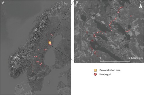
Coordinates of 2000 known hunting pits were downloaded from the Swedish national heritage board (Figure 1A). The coordinates were manually adjusted based on visual observations in a hill-shaded elevation model. The area surrounding known hunting pits was inspected, and additional hunting pits were manually digitized if discovered. The adjusted coordinates were also converted to polygon circles outlining the size of each hunting pit. In total, 2519 hunting pits were digitized in this way. These polygons were converted into segmentation masks where pixels inside the polygons were given a value of 1 and pixels outside the polygons were given a value of 0. The segmentation masks were also converted to bounding boxes for the YOLO model.

Figure 1. Locations of hunting pits used in this study. In total, 2519 hunting pits were manually mapped in northern Sweden. Some 80% of the hunting pits were used for training the models, while 20% were used for testing.

Topographical indices

A compact laser-based system (Leica ALS80-HP-8236) was used to collect the ALS data from an aircraft flying at 2888–3000 m. The ALS point clouds had a point density of 1–2 points m² and were divided into 204 tiles with a size of 2.5 × 2.5 km each. The tiles covered an area of 1275 km². DEMs with 0.5 m and 1 m resolution were created from the ALS point clouds using a TIN gridding approach implemented in Whitebox tools 2.2.0 (Lindsay 2016). Ten topographical indices were calculated from the DEMs using Whitebox Tools to highlight local topography, making it easier for the deep learning model to learn how hunting pits appear in the DEMs.

The first was multidirectional hill shading, a process that combines hill-shaded images from azimuth positions at 225, 270, 315, and 360 (0) degrees. The amalgamation of these images is achieved through a weighted summation, with azimuth positions at 270 degrees holding the highest weight of 0.4, followed by positions at 225 and 315 degrees with weights of 0.1 each, and finally, 360 (0) degrees with a weight of 0.1.

Moving on, the maximum elevation deviation measures the maximum deviation from mean elevation for each grid cell in a DEM across various spatial scales. This multiscale analysis is densely sampled and quantifies the relative topographic position as a fraction of local relief normalized to the local surface roughness, as proposed by Lindsay, Cockburn, and Russell (2015).

Another topographical index included was the multiscale elevation percentile, a metric that calculates the greatest elevation percentile across a range of spatial scales. This measurement serves to express the local topographic position, representing the vertical position for each DEM grid cell as a percentile of the elevation distribution, as outlined by Huang, Yang, and Tang (1979) and Newman, Lindsay, and Cockburn (2018).

The analysis also delves into curvature measures, distinguishing between minimal and maximal curvature. Minimal curvature indicates the curvature of a principal section with the lowest value at a given point on the topographic surface, where positive values denote hills and negative values suggest valley positions. Conversely, maximal curvature represents the curvature of a principal section with the highest value at a given point on the surface, with positive values signifying ridge positions and negative values indicating closed depressions, according to the work of Shary, Sharaya, and Mitusov (2002).

Profile curvature, another parameter, is examined as the curvature of a normal section having a common tangent line with a slope line at a given point on the surface. Positive values of the index are indicative of flow acceleration, while negative profile curvature values indicate flow deceleration, following the principles outlined by Shary, Sharaya, and Mitusov (2002).

Further, the analysis incorporates measures of surface shape complexity, texture, and roughness, such as the spherical standard deviation of normal. This metric quantifies the angular dispersion of surface normal vectors within a local neighborhood, utilizing a specified filter window of 11 pixels in this study, as established by Grohmann, Smith, and Riccomini (2011), Hodgson and Gaile (1999), and Lindsay, Newman, and Francioni (2019).

Moreover, a multiscale standard deviation of normal is introduced, akin to the spherical standard deviation of normal but extending its applicability across multiple scales without necessitating a specified filter window. The analysis also includes elevation above pit, which calculates the elevation of each grid cell in a DEM above the nearest downslope pit cell along the flow path. Additionally, depth in sink is explored as a measure of the depth of each grid cell within a closed topographic depression, defined as a bowl-like landscape feature without an outlet, as proposed by Antonić, Hatic, and Pernar (2001).

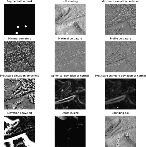
The topographical indices and labelled images from the 204 tiles were split into image chips with 250 × 250 pixels in each chip (Figure 2). Image chips without hunting pits were removed to combat the highly imbalanced class distribution. This resulted in 1640 image chips with 0.5 m DEM and 1023 image chips from the 1 m DEM. Some 80% of the chips were randomly selected for training and 20% for testing. Further, we assumed that the hunting pits and the immediate surrounding terrain did not have any preferred orientation, which allowed for image augmentation by rotating and flipping the image chips during training.

Figure 2. An example of one of the image chips used to train the deep learning models. Each topographical index was selected to highlight the local topography to make it easier for the deep learning model to learn how hunting pits appear in the lidar data. The segmentation mask was used as the label for the segmentation model, while the bounding boxes were used for the object detection model. The chips displayed here are from a DEM with 0.5 m resolution.

Transfer learning

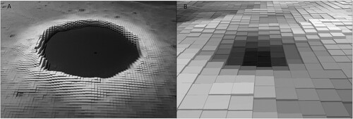
Due to the relatively small number of digitized hunting pits, we chose to utilize transfer learning, i.e. training on similar data from another data source, before fine-tuning the model on the real data. Inspired by recent work by Gallwey and colleagues (2019), we chose to use impact craters on the lunar surface as a transfer learning strategy. The idea was that impact craters are pits in a lunar DEM and so would be similar enough to hunting pits on Earth to give our models a better starting point than random initialized weights (Figure 3). The craters were digitized by NASA and were available from the Moon Crater Database v1 (Robbins 2019). The database contained approximately 1.3 million lunar impact craters and were approximately complete for all craters larger than about 1–2 km in diameter. Craters were manually identified and measured with data from the Lunar Reconnaissance Orbiter (LRO). The Lunar Orbiter Laser Altimeter, which was located on the LRO spacecraft, was used to create a DEM of the moon with a resolution of 118 m (Mazarico et al. 2012). All models were pre-trained with the lunar data before being trained on the hunting pit dataset.

Figure 3. A) An example of an impact crater in the lunar DEM. Each pixel in the DEM is 118 × 118 m. B) A hunting pit in a DEM created from the national lidar point cloud from Sweden. Each pixel is 0.5 × 0.5 m.

Deep learning architectures

This study evaluated three deep learning architectures: semantic segmentation using two types of U-nets, a standard U-net and an Xception U-net, as well as object detection using a variant of “You Only Look Once (YOLO)” called You Only Learn One Representation (YOLOR).

Semantic segmentation

We used TensorFlow 2.6 to build two types of encoder-decoder style deep neural networks to transform the topographical indices into images highlighting the detected hunting pits. On the encoding path, the networks learn a series of filters, organized in layers, which express larger and larger neighborhoods of pixels in fewer and fewer vectors of features. This downsampling forces the networks to ignore noise and extract features relevant for hunting pit detection. In addition to this regular U-net, which applies a filter to all feature vectors in a specific spatial neighborhood at once, we also used a U-net with Xception blocks (Chollet 2017), which we refer to as Xception UNet. These blocks decouple the filtering of the spatial neighborhood within each feature dimension from the filtering across feature dimensions. This approach simplifies the learning problem for hunting pit detection, since there is no strong coupling between the two dimensions. After encoding the images into a spatially more compact representation, it is again decoded by a series of learned filters carrying out transposed convolutions into the final classification map. This map contains, for every pixel in the input image, the probability that the pixel belongs to a hunting pit. Since only about 1% of the pixels in the input images were labelled as hunting pits, we used a focal loss function to increase their weight during training (Lin et al. 2017). Since segmentation models output a probability for each individual pixel instead of objects as YOLOR does, we chose to merge neighboring pixels into polygons which could be intersected with the digitized hunting pits for evaluation.

Object detection

YOLOR is an object detection model that attempts to find objects in images rather than classify individual pixels as U-net does. The architecture uses convolutional filters that extract features into channels. We used the YOLOR implementation from Wang, Yeh, and Liao (2021). YOLOR outputs bounding boxes with a probability metric for each. In this study, we selected bounding boxes with a probability of 85% for evaluation.

Evaluation

Model performance was evaluated both quantitatively and qualitatively. Some 80% of the image chips were used to train the model and 20% to test the models. A centroid-based approach described by Fiorucci and colleagues (2022) was used to calculate the number of true positive, false positive, and false negative predicted hunting pits. These numbers were then used to calculate recall, precision, and F1 score for each model. The F1 score symmetrically represents both precision and recall in one metric, and the most accurate model was selected as the one with the highest F1 score. The most accurate models for each resolution were used to map hunting pits in a demonstration area in northern Sweden where 80 hunting pits had been mapped manually (Figure 1B) This was done in order to inspect the results visually, in addition to the statistical metrics from the test data. To evaluate the feasibility of implementing these models on large scales, we also calculated the processing time that each combination of topographical index and deep learning model needed for predicting hunting pits per km².

Results

Three deep learning architectures were evaluated for 10 different topographical indices extracted from DEMs with two resolutions. The U-net model trained on the topographical index profile curvature from a 0.5 m DEM was the most accurate method, with an F1 score of 0.76. This method was able to map 70% of all hunting pits and had a false positive rate of 15% when evaluated on the test data.

Performance with test data

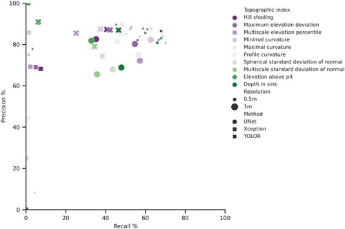
The evaluation was carried out in two parts. First, the performance using the 20% test data that had been set aside was assessed. Second, the best combination of DEM resolution and topographical index was applied to a separate demonstration area for visual inspection. The models that were trained on topographical indices from a 0.5 m DEM were more accurate than models trained on topographical indices from a 1 m DEM, shown as higher recall and precision in Figure 4. Further, both the standard U-net and the XceptionUNet proved to be more accurate with the test data than YOLOR, regardless of resolution, although Xception UNet tended to lead to higher precision while the standard U-net led to higher recall. All topographical indices worked fairly well for both segmentation models, but the curvature-based indices (minimal, maximal, and profile-curvature) resulted in models with slightly better performance in terms of F1 score. The YOLOR models showed more variation across the topographical indices, with hill shading, maximum elevation deviation, and maximal curvature being the best.

Figure 4. Results from the models when evaluated with the test data. Recall is defined as how many of all the hunting pits in the test data each model can map. Precision is defined as how many of the predicted hunting pits are actual hunting pits. Both these metrics should be high for a reliable model.

There were also large differences in how much time each combination of topographical index and deep learning architecture required to move from a raw DEM to mapped hunting pits. This time includes both the processing time of the topographical indices and the inference time of the deep learning model (Figure 5). The major difference in processing time is between the 0.5 m DEM and 1 m DEM, since changing from a resolution of 1 m to 0.5 m increases the number of pixels by a factor of four. The difference in F1 score between the best model from a 0.5 m DEM (UNet on profile curvature) and the best model from a 1 m DEM (UNet on minimal curvature) was a small decrease from 0.76 to 0.71. If these models were to be implemented on all forest land in Sweden, the processing time would be 241 days on a 0.5 m DEM and 55 days on a 1 m DEM when running on a single graphics processing unit (NVIDIA A100 GPU). However, this is a highly parallelizable problem, so the processing could be spread across multiple GPUs in a computer cluster. Although it was difficult to compare these results with the models developed and tested using different landscapes and with different ALS data, the metrics of our best model were on par with or better than previous studies. Different studies presented different metrics; the most commonly used metrics are summarized in Table 1.

Figure 5. F1 score plotted against processing time. The high-resolution data requires more processing time due to an increase in the number of pixels.

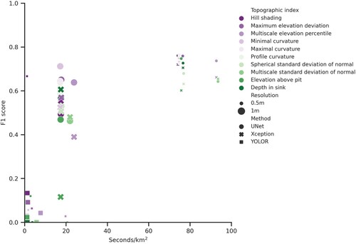
Table 1. Performance with the test data compared to published approaches of mapping hunting pits. Point density refers to the ALS point cloud used to train and test the methods.

Study	Recall	Precision	F1 score	Point density
Present study (Unet 0.5 m)	70	85	0.76	1–2
Trier and Pilø (2012)	67–76	-	-	7
Trier, Reksten, and Løseth (2021)	86	80	0.83	5–12
Seitsonen and Ikäheimo (2021)	98	47	0.64	5

Performance for the demonstration area

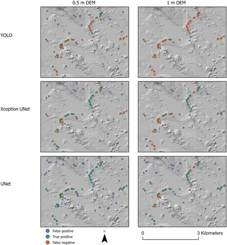
In addition to the quantitative evaluation with the test data, we also implemented the best models for each resolution in northern Sweden where a system of hunting pits had been manually mapped (Figure 6). YOLOR failed to map most of the hunting pits in the area, regardless of resolution. The Xception UNet mapped more hunting pits than YOLOR, while the UNet model captured most of the hunting pits of all models but also had the highest number of false positives.

Figure 6. Example from the demonstration area in northern Sweden where a system of manually mapped hunting pits can be seen as two main arches from southwest to northeast. There were also some hunting pits on ridges (green and red points). Each model used the best topographical index for each resolution.

Discussion

For this study, we analyzed and made openly available a large dataset of 2519 mapped hunting pits spread across 1275 km² in a landscape mainly dominated by forest. The total area of forest land in Sweden is 280,000 km². In addition to our own analysis, this dataset can be used for pre-training future models in the same manner as the moon was used in this study. Further, we demonstrated that our approach of combining deep learning with high-density ALS data to map hunting pits has accuracy close to, or equal to, that of previous studies.

Point density of ALS data

One of the research questions in this study was to investigate whether the point density of the national Swedish ALS data (1–2 points/m²) is enough to map small-scale cultural remains such as hunting pits. Gallagher and Josephs (2008) argued that there is a very strong relationship between the size of cultural remains and the detection success rates. Their results estimated that as many as 90% of the cultural remains larger than 16 m in diameter can be expected to be successfully detected. Some 41% of remains between 12 and 16 m in size were successfully detected, with a large drop to less than 9% for those measuring less than 12 m in size. This will also depend on the point density in the ALS data and DEM resolution. Hunting pits are only a few meters in diameter, and Opitz and Herrmann (2018) noted that the major weakness of automatic methods are that they are not applicable for detection of archaeological features with heterogeneous backgrounds at a large scale. However, Trier, Reksten, and Løseth (2021) demonstrated that it is possible to train accurate models that can detect small features such as hunting pits with denser ALS point clouds. While the best model presented in our study had 15% false detections, it still managed to detect 70% of all hunting pits in our test data using the Swedish ALS data with only 1–2 points/m². Trier and Pilø (2012) investigated the relationship between human detection rates and ALS point density and concluded that 1.8 ground returns/m² were required for human experts to detect hunting pits visually at a recall of 82%. This puts our model slightly below human experts in terms of recall. Trier and Pilø (2012) argued that at least 2.5 pulses per m² are required as a minimum. It is reasonable to assume that the deep learning methods would perform better with a higher point density, which stresses the need for more dense ALS data to increase the detection rate of small-scale archaeological features.

Topographical terrain indices

Another aim of this study was to evaluate the performance of different topographical indices (including traditional indices such as hill shading but also recently-developed scale-optimized surface roughness methods such as spherical standard deviation of the distribution of surface normal and multiscale elevation percentile) for mapping hunting pits with deep learning. However, we only observed small differences in performance across these topographical indices. This suggests that this kind of feature engineering is not crucial for mapping cultural remains with high-resolution ALS data. The deep learning models learn enough features using their convolution filters. In fact, a possible reason as to why the multiscale indices and the spherical standard deviation of normal indices performed worse could be that they lose too much information when combining different scales when the features we are trying to map are of the same local scale. Multiscale analytical techniques are probably more useful to map cultural remains that have a larger variation in scale than hunting pits.

The low precision in our model (15% of all detected pits are false positives) can be partly attributed to other types of pits found in the landscape. The models in this study are good tools for mapping pit-like features in the landscape, but not all pits are hunting pits. There are both anthropogenic and natural depressions that can be mistaken for hunting pits, and the point density of the Swedish ALS data was probably not high enough to separate them. Trier, Reksten, and Løseth (2021) suggested that citizen science projects could be used as a way to visually verify detected hunting pits but also mentioned that experts might be needed for a proper identification. Another way of distinguishing hunting pits from other pits without manual verification or costly archaeological field investigations is to study the spatial context in which they appear, i.e. the mutual relationships between the pits and their location in the landscape. Usually, a precondition for studying such relationships is the ability to work with large landscape areas, since catching systems can consist of hundreds of hunting pits and stretch for several kilometers. A possible way to achieve this is to add a post-processing step where decision tree-based methods are used to separate detected pits based on, for example, soil type and distance to other pits. This step could reduce the number of false positives when the model is implemented on a regional or national scale. Other considerations for large-scale implementations are trade-offs between processing time and accuracy. The best model trained on a DEM with 0.5 m resolution had an F1 score of 0.76 and recall of 70% compared to an F1 score of 0.71 and recall of 63% using a 1 m DEM. Depending on the application and scale, this decrease in accuracy might be worth considering, given that the number of pixels that have to be processed is reduced by a factor of four.

Policy implications

Due to the urgent need to detect and protect cultural remains in the forest landscape before they are destroyed by forestry activity or other forms of modern land use, it is of interest to all the involved actors that new decision support tools are developed. However, it is also important to understand and discuss the potential implications of these tools for policy and practice. As our study has shown, utilizing machine learning as tools in forestry to detect ancient monuments presents both benefits and risks. Besides the evident benefits such as a potential for increasing the degree of detection and documentation of ancient monuments with the potential to aid in forest planning and management, these methods can also enhance the efficiency in the analysis of large datasets compared to manual methods (Opitz and Herrmann 2018; Soroush et al. 2020). However, the time used to prepare a deep learning approach and interpret the results, as well as the need to do subsequent field-verifications, should not be underestimated.

However, there are also several risks associated with the application, since the algorithms—as we have seen—may occasionally misidentify natural features as cultural remains or vice versa, thus failing to recognize actual remains, which may result in misinterpretations and the potential loss of significant sites (Verschoof-van der Vaart et al. 2020). Since the algorithms used are trained on existing data, this can introduce biases from previous research or incomplete datasets and thus reduce the accuracy of detection. This became particularly visible in our study where some smaller features, such as individual hunting pits, were not properly detected. This makes hunting pits a good example of the challenges with using machine learning and ALS data to detect small-scale archaeological features. Since the Swedish ALS data only contain 1–2 points /m², there is a risk that smaller features are discriminated against in favor of larger features that are easier to detect. At the same time, a very evident benefit is that the data we can provide and deliver from our model are directly useful in forestry planning and can be directly incorporated into the maps already used for logging machines and machines undertaking soil scarification. Previous work in forest water (Lidberg, Nilsson, and Ågren 2020; Lidberg et al. 2023) has proven that such maps can have an immediate effect on forest management, even if the maps fail to capture all cultural features.

Conclusions

Mapping cultural remains such as hunting pits is an important first step to ensure their protection in accordance with the Cultural Environment Act. We showed that semantic image segmentation with deep learning from high-resolution ALS data can be used to detect 70% of hunting pits in Sweden. However, 15% of all detected hunting pits were, in fact, false positives. Most topographical indices explored in this study worked well, and the main increase in performance came from increasing the resolution of the DEM from 1 m to 0.5 m. Denser ALS point clouds would likely improve the performance of all models and reduce the risks associated with large-scale applications.

Open Scholarship

This article has earned the Center for Open Science badges for Open Data and Open Materials through Open Practices Disclosure. The data and materials are openly accessible at https://doi.org/10.5878/en98-1b29 and https://doi.org/10.5878/en98-1b29.

Data Reproducibility

Figures 4 and 5 of this manuscript, as well as the model performance output presented in Table 1, prepared by the author, were successfully reproduced in an independent process by the JFA’s Associate Editor for Reproducibility.

Acknowledgements

We thank the Swedish Forest Agency for digitizing part of the hunting pits used in this study. This work was partially supported by the Wallenberg AI, Autonomous Systems and Software Program—Humanities and Society (WASP-HS) funded by the Marianne and Marcus Wallenberg Foundation, the Marcus and Amalia Wallenberg Foundation, Kempestiftelserna, and the Swedish forest agency.

Data Availability

Data, models, and code generated or used during the study are available in a repository online in accordance with funder data retention policies. The code and trained models are available from Github (Lidberg 2023), and the data used in this study is available (Lidberg 2024).

Additional information

Notes on contributors

William Lidberg

William Lidberg (Ph.D. 2019, Swedish University of Agricultural Sciences) is an assistant professor in soil science. His research focuses on mapping small-scale features in the forest landscape using geographical data and machine learning.

Florian Westphal

Florian Westphal (Ph.D. 2020, Blekinge Institute of Technology) is an assistant professor in computer science. His research interest is focused on guided, or interactive, machine learning, which aims at developing mechanisms to allow non-machine learning experts to adapt intelligent systems to local contexts.

Christoffer Brax

Christoffer Brax (Ph.D. 2003, Umeå University) is a computer scientist at Combitech and is currently working with the Swedish Forest Agency.

Camilla Sandström

Camilla Sandström (Ph.D. 2003, Umeå University) is a professor in political science and Chairholder, UNESCO chair on biosphere reserves as labs for inclusive societal transformation. Her research is focused on the governance and management of natural resources.

Lars Östlund

Lars Östlund (Ph.D. 1994, Swedish University of Agricultural Sciences) is a professor in forest ecology, specializing in forest history. His research is focused on the cultural history of boreal forests in Scandinavia, the US, and Chile, logging history, and fire ecology in Scandinavia.

References

- Agnoletti, M., and A. Santoro. 2018. “Rural Landscape Planning and Forest Management in Tuscany (Italy).” Forests 9 (8): 473. https://doi.org/10.3390/f9080473.
- Amréus, L. 2020. Skador på Fornlämningar och övriga Kulturhistoriska Lämningar vid Skogsbruk. Riksantikvarieämbetet. https://urn.kb.se/resolve?urn=urn:nbn:se:raa:diva-6082.
- Antonić, O., D. Hatic, and R. Pernar. 2001. “DEM-Based Depth in Sink as an Environmental Estimator.” Ecological Modelling 138 (1): 247–54. https://doi.org/10.1016/S0304-3800(00)00405-1.
- Caspari, G. 2023. “The Potential of New LiDAR Datasets for Archaeology in Switzerland.” Remote Sensing 15 (6): 1569. https://doi.org/10.3390/rs15061569.
- Caspari, G., and P. Crespo. 2019. “Convolutional Neural Networks for Archaeological Site Detection – Finding “Princely” Tombs.” Journal of Archaeological Science 110 (October): 104998. https://doi.org/10.1016/j.jas.2019.104998.
- Chollet, F. 2017. “Xception: Deep Learning with Depthwise Separable Convolutions.”.
- Fiorucci, M., W. B. Verschoof-van der Vaart, P. Soleni, B. Le Saux, and A. Traviglia. 2022. “Deep Learning for Archaeological Object Detection on LiDAR: New Evaluation Measures and Insights.” Remote Sensing 14 (7): 1694. https://doi.org/10.3390/rs14071694.
- Freeland, T., B. Heung, D. V. Burley, G. Clark, and A. Knudby. 2016. “Automated Feature Extraction for Prospection and Analysis of Monumental Earthworks from Aerial LiDAR in the Kingdom of Tonga.” Journal of Archaeological Science 69 (May): 64–74. https://doi.org/10.1016/j.jas.2016.04.011.
- Gallagher, J. M., and R. L. Josephs. 2008. “Using LiDAR to Detect Cultural Resources in a Forested Environment: An Example from Isle Royale National Park, Michigan, USA.” Archaeological Prospection 15 (3): 187–206. https://doi.org/10.1002/arp.333.
- Gallwey, J., M. Eyre, M. Tonkins, and J. Coggan. 2019. “Bringing Lunar LiDAR Back Down to Earth: Mapping Our Industrial Heritage Through Deep Transfer Learning.” Remote Sensing 11 (17): 1994. https://doi.org/10.3390/rs11171994.
- Grohmann, C. H., M. J. Smith, and C. Riccomini. 2011. “Multiscale Analysis of Topographic Surface Roughness in the Midland Valley, Scotland.” IEEE Transactions on Geoscience and Remote Sensing 49 (4): 1200–1213. https://doi.org/10.1109/TGRS.2010.2053546.
- Guyot, A., M. Lennon, T. Lorho, and L. Hubert-Moy. 2021. “Combined Detection and Segmentation of Archeological Structures from LiDAR Data Using a Deep Learning Approach.” Journal of Computer Applications in Archaeology 4 (1): 1. https://doi.org/10.5334/jcaa.64.
- Hennius, A. 2020. “Towards a Refined Chronology of Prehistoric Pitfall Hunting in Sweden.” European Journal of Archaeology 23 (4): 530–46. https://doi.org/10.1017/eaa.2020.8.
- Hodgson, M., and G. Gaile. 1999. “A Cartographic Modeling Approach for Surface Orientation-Related Applications.” Photogrammetric Engineering and Remote Sensing. https://www.semanticscholar.org/paper/A-Cartographic-Modeling-Approach-for-Surface-Hodgson-Gaile/acfeaeeab769cd2892a04782f5fec6dca84c1d21.
- Huang, T., G. Yang, and G. Tang. 1979. “A Fast Two-Dimensional Median Filtering Algorithm.” IEEE Transactions on Acoustics, Speech, and Signal Processing 27 (1): 13–18. https://doi.org/10.1109/TASSP.1979.1163188.
- Ibrahim, Y., B. Nagy, and C. Benedek. 2019. “CNN-Based Watershed Marker Extraction for Brick Segmentation in Masonry Walls.” In Image Analysis and Recognition, Iciar 2019, Pt I, edited by F. Karray, A. Campilho, and A. Yu, 11662:332–44. Cham: Springer International Publishing Ag. https://doi.org/10.1007/978-3-030-27202-9_30.
- Johnson, K. M., and W. B. Ouimet. 2014. “Rediscovering the Lost Archaeological Landscape of Southern New England Using Airborne Light Detection and Ranging (LiDAR).” Journal of Archaeological Science 43 (March): 9–20. https://doi.org/10.1016/j.jas.2013.12.004.
- Li, N., Z. Guo, J. Zhao, L. Wu, and Z. Guo. 2022. “Characterizing Ancient Channel of the Yellow River from Spaceborne SAR: Case Study of Chinese Gaofen-3 Satellite.” Ieee Geoscience and Remote Sensing Letters 19: 1502805. https://doi.org/10.1109/LGRS.2021.3116693.
- Lidberg, W. 2023. “Detection of Hunting Pits Using Airborne Laser Scanning and Deep Learning.” https://github.com/williamlidberg/Detection-of-hunting-pits-using-airborne-laser-scanning-and-deep-learning.
- Lidberg, W. 2024. “Detection of Hunting Pits Using Airborne Laser Scanning and Deep Learning (Version 1) [Data set].” Swedish University of Agricultural Sciences. Available at: https://doi.org/10.5878/en98-1b29.
- Lidberg, W., M. Nilsson, and A. Ågren. 2020. “Using Machine Learning to Generate High-Resolution Wet Area Maps for Planning Forest Management: A Study in a Boreal Forest Landscape.” Ambio 49 (2), https://doi.org/10.1007/s13280-019-01196-9.
- Lidberg, W., S. S. Paul, F. Westphal, K. F. Richter, N. Lavesson, R. Melniks, J. Ivanovs, M. Ciesielski, A. Leinonen, and A. M. Ågren. 2023. “Mapping Drainage Ditches in Forested Landscapes Using Deep Learning and Aerial Laser Scanning.” Journal of Irrigation and Drainage Engineering 149 (3): 04022051. https://doi.org/10.1061/JIDEDH.IRENG-9796.
- Liedgren, L., G. Hörnberg, T. Magnusson, and L. Östlund. 2017. “Heat Impact and Soil Colors Beneath Hearths in Northern Sweden.” Journal of Archaeological Science 79 (March): 62–72. https://doi.org/10.1016/j.jas.2017.01.012.
- Lin, T.-Y., P. Goyal, R. Girshick, K. He, and P. Dollár. 2017. “Focal Loss for Dense Object Detection.” arXiv.Org. 7 August 2017. https://arxiv.org/abs/1708.02002v2.
- Lindsay, J. B. 2016. “Whitebox GAT: A Case Study in Geomorphometric Analysis.” Computers & Geosciences 95 (October): 75–84. https://doi.org/10.1016/j.cageo.2016.07.003.
- Lindsay, J. B., J. M. H. Cockburn, and H. A. J. Russell. 2015. “An Integral Image Approach to Performing Multi-Scale Topographic Position Analysis.” Geomorphology 245 (September): 51–61. https://doi.org/10.1016/j.geomorph.2015.05.025.
- Lindsay, J. B., D. R. Newman, and A. Francioni. 2019. “Scale-Optimized Surface Roughness for Topographic Analysis.” Geosciences 9 (7): 322. https://doi.org/10.3390/geosciences9070322.
- Luo, Lei, Xinyuan Wang, Huadong Guo, R. Lasaponara, Xin Zong, N. Masini, Guizhou Wang, et al. 2019. “Airborne and Spaceborne Remote Sensing for Archaeological and Cultural Heritage Applications: A Review of the Century (1907–2017).” Remote Sensing of Environment 232 (October): 111280. https://doi.org/10.1016/j.rse.2019.111280.
- Mazarico, E., D. D. Rowlands, G. A. Neumann, D. E. Smith, M. H. Torrence, F. G. Lemoine, and M. T. Zuber. 2012. “Orbit Determination of the Lunar Reconnaissance Orbiter.” Journal of Geodesy 86 (3): 193–207. https://doi.org/10.1007/s00190-011-0509-4.
- Newman, D. R., J. B. Lindsay, and J. M. H. Cockburn. 2018. “Evaluating Metrics of Local Topographic Position for Multiscale Geomorphometric Analysis.” Geomorphology 312 (July): 40–50. https://doi.org/10.1016/j.geomorph.2018.04.003.
- Norstedt, G., A.-L. Axelsson, H. Laudon, and L. Östlund. 2020. “Detecting Cultural Remains in Boreal Forests in Sweden Using Airborne Laser Scanning Data of Different Resolutions.” Journal of Field Archaeology 45 (1): 16–28. https://doi.org/10.1080/00934690.2019.1677424.
- Opitz, R., and J. Herrmann. 2018. “Recent Trends and Long-Standing Problems in Archaeological Remote Sensing.” Journal of Computer Applications in Archaeology 1 (1): 19–41. https://doi.org/10.5334/jcaa.11.
- Ögren, F. 2019. “Hantering av forn- och kulturlämningar inom SCA Norrbottens skogsförvaltning.” Second cycle, A2E. Umeå: SLU, Dept. of Forest Ecology and Management. 11 September 2019. https://stud.epsilon.slu.se/15028/.
- Östlund, L., O. Zackrisson, and A.-L. Axelsson. 1997. “The History and Transformation of a Scandinavian Boreal Forest Landscape Since the 19th Century.” Canadian Journal of Forest Research 27 (8): 1198–1206. https://doi.org/10.1139/x97-070.
- Raymond, G. 2022. “Skador på kultur- och fornlämningar i samband med förynringsaverkning - med fokus på oregisterade lämningar.” Alnarp: Swedish University of Agricultural Science. https://stud.epsilon.slu.se/18236/.
- Redmon, J., S. Divvala, R. Girshick, and A. Farhadi. 2016. “You Only Look Once: Unified, Real-Time Object Detection.” arXiv, https://doi.org/10.48550/arXiv.1506.02640.
- Reutebuch, S. E., H.-E. Andersen, and R. J. McGaughey. 2005. “Light Detection and Ranging (LIDAR): An Emerging Tool for Multiple Resource Inventory.” Journal of Forestry 103 (6): 286–92. https://doi.org/10.1093/jof/103.6.286.
- Robbins, S. J. 2019. “A New Global Database of Lunar Impact Craters >1–2 Km: 1. Crater Locations and Sizes, Comparisons with Published Databases, and Global Analysis.” Journal of Geophysical Research: Planets 124 (4): 871–92. https://doi.org/10.1029/2018JE005592.
- Ronneberger, O., P. Fischer, and T. Brox. 2015. “U-Net: Convolutional Networks for Biomedical Image Segmentation.” In Medical Image Computing and Computer-Assisted Intervention – MICCAI 2015, edited by N. Navab, J. Hornegger, W. M. Wells, and A. F. Frangi, 234–41. Lecture Notes in Computer Science. Cham: Springer International Publishing. https://doi.org/10.1007/978-3-319-24574-4_28.
- Seitsonen, O., and J. Ikäheimo. 2021. “Detecting Archaeological Features with Airborne Laser Scanning in the Alpine Tundra of Sápmi, Northern Finland.” Remote Sensing 13 (8): 1599. https://doi.org/10.3390/rs13081599.
- Shary, P. A., L. S. Sharaya, and A. V. Mitusov. 2002. “Fundamental Quantitative Methods of Land Surface Analysis.” Geoderma 107 (1): 1–32. https://doi.org/10.1016/S0016-7061(01)00136-7.
- Soroush, M., A. Mehrtash, E. Khazraee, and J. A. Ur. 2020. “Deep Learning in Archaeological Remote Sensing: Automated Qanat Detection in the Kurdistan Region of Iraq.” Remote Sensing 12 (3): 500. https://doi.org/10.3390/rs12030500.
- Štular, B., Ž Kokalj, K. Oštir, and L. Nuninger. 2012. “Visualization of Lidar-Derived Relief Models for Detection of Archaeological Features.” Journal of Archaeological Science 39 (11): 3354–60. https://doi.org/10.1016/j.jas.2012.05.029.
- Thuestad, A. E., O. Risbøl, J. I. Kleppe, S. Barlindhaug, and E. R. Myrvoll. 2021. “Archaeological Surveying of Subarctic and Arctic Landscapes: Comparing the Performance of Airborne Laser Scanning and Remote Sensing Image Data.” Sustainability 13 (4): 1917. https://doi.org/10.3390/su13041917.
- Trier, ØD, D. C. Cowley, and A. U. Waldeland. 2019. “Using Deep Neural Networks on Airborne Laser Scanning Data: Results from a Case Study of Semi-Automatic Mapping of Archaeological Topography on Arran, Scotland.” Archaeological Prospection 26 (2): 165–75. https://doi.org/10.1002/arp.1731.
- Trier, ØD, and L. H. Pilø. 2012. “Automatic Detection of Pit Structures in Airborne Laser Scanning Data: Automatic Detection of Pits in ALS Data.” Archaeological Prospection 19 (2): 103–21. https://doi.org/10.1002/arp.1421.
- Trier, ØD, J. H. Reksten, and K. Løseth. 2021. “Automated Mapping of Cultural Heritage in Norway from Airborne Lidar Data Using Faster R-CNN.” International Journal of Applied Earth Observation and Geoinformation 95 (March): 102241–102241. https://doi.org/10.1016/j.jag.2020.102241.
- Trier, ØD, M. Zortea, and C. Tonning. 2015. “Automatic Detection of Mound Structures in Airborne Laser Scanning Data.” Journal of Archaeological Science: Reports 2 (June): 69–79. https://doi.org/10.1016/j.jasrep.2015.01.005.
- Verschoof-van der Vaart, W. B., and K. Lambers. 2019. “Learning to Look at LiDAR: The Use of R-CNN in the Automated Detection of Archaeological Objects in LiDAR Data from the Netherlands.” Journal of Computer Applications in Archaeology 2 (1): 31–40. https://doi.org/10.5334/jcaa.32.
- Verschoof-van der Vaart, W. B., K. Lambers, W. Kowalczyk, and Q. P. J. Bourgeois. 2020. “Combining Deep Learning and Location-Based Ranking for Large-Scale Archaeological Prospection of LiDAR Data from The Netherlands.” ISPRS International Journal of Geo-Information 9 (5): 293. https://doi.org/10.3390/ijgi9050293.
- Wang, C.-Y., I.-H. Yeh, and H.-Y. M. Liao. 2021. “You Only Learn One Representation: Unified Network for Multiple Tasks.” arXiv, https://doi.org/10.48550/arXiv.2105.04206.
- Yang, F. 2021. “An Improved YOLO v3 Algorithm for Remote Sensing Image Target Detection.” Journal of Physics: Conference Series 2132 (1): 012028. https://doi.org/10.1088/1742-6596/2132/1/012028.