The effect of number of clusters and cluster size on statistical power and Type I error rates when testing random effects variance components in multilevel linear and logistic regression models

Abstract

When using multilevel regression models that incorporate cluster-specific random effects, the Wald and the likelihood ratio (LR) tests are used for testing the null hypothesis that the variance of the random effects distribution is equal to zero. We conducted a series of Monte Carlo simulations to examine the effect of the number of clusters and the number of subjects per cluster on the statistical power to detect a non-null random effects variance and to compare the empirical type I error rates of the Wald and LR tests. Statistical power increased with increasing number of clusters and number of subjects per cluster. Statistical power was greater for the LR test than for the Wald test. These results applied to both the linear and logistic regressions, but were more pronounced for the latter. The use of the LR test is preferable to the use of the Wald test.

Keywords:

• Statistical power
• multilevel analysis
• multilevel model
• hierarchical model
• variance components

1. Introduction

Data with a multilevel nature occur frequently in education, public health, health services research, behavioural research, and in social epidemiology. Examples include patients nested within primary care practices, students nested within schools, and employees nested within companies. A consequence of the clustering of subjects within clusters (e.g. patients clustered within primary care practices) is that subjects from the same cluster may have outcomes that are more similar than will subjects from different clusters. Researchers are increasingly using multilevel regression models to analyse clustered data [1,2]. Multilevel regression models incorporate cluster-specific random effects that account for the dependency of the data by partitioning the total individual variance into variation due to the cluster and the individual-level variation that remains [3].

An important question when analysing multilevel data is whether clustering exerts an effect on subject outcomes. Formal statistical testing of the hypothesis that the variance of the distribution of the random effects is equal to zero permits one to assess whether clustering exerts an effect on the outcome. Two different statistical tests are used frequently to test this hypothesis: the Wald test and the likelihood ratio test [4–6]. Molenberghs and Verbeke reviewed these tests, presented their asymptotic equivalence and showed how to compute their p-values taking into account the one-sided nature of variance testing [4]. Considering various statistical and computational considerations, their pragmatic guideline is that the likelihood ratio test is ‘the easiest to evaluate’ (p.27) and they recommend to ‘consider it the default’ (p.27). However, they acknowledge ‘we do not claim to have provided a definitive answer, for which both additional small sample and asymptotic evaluations, accompanied with simulations, would be needed’ (p.27). The objective of the current paper is to fill this void with a comprehensive simulation study of small-sample settings. First, we investigate the effect of the number of clusters and the number of subjects per cluster on the statistical power to detect a non-zero random effects variance. Second, we compare the type I error rate of the Wald test and the likelihood ratio test. We examine testing the random effects variance for both the linear random effects model for use with continuous outcomes and the logistic regression random effects model for use with binary outcomes.

The paper is structured as follows. In Section 2, we describe the regression models that we consider. We also describe the Wald and the likelihood ratio tests for testing whether the variance of the random effects distribution is equal to zero. In Section 3, we provide an extensive series of Monte Carlo simulations to address our study objectives. Finally, in Section 4, we summarize our findings.

2. Notation and statistical tests for null variance

In this section, we formally describe the linear and logistic random effects models under consideration. We then describe the Wald and likelihood ratio tests that have been proposed for testing whether the variance of the distribution of the random effects is statistically significantly different from zero.

2.1. The linear and logistic random effects models

2.1.1. The linear random effects model

Let $Y_{ij}$ denote a continuous outcome measured on the ith subject in the jth cluster. Let (1) $Y_{ij}={\alpha }_0+{\alpha }_{0j}+{\alpha }_1{X}_{1ij}+{\alpha }_2{X}_{2ij}+\cdots +{\alpha }_k{X}_{kij}+{\epsilon }_{ij}$(1) where ${\alpha }_{0j}\sim N(0,{\tau }^2)$ and ${\epsilon }_{ij}\sim N(0,{\sigma }^2)$ describe a linear model in which the continuous outcome variable is regressed on k predictor variables (X₁,  … , X_k). The model incorporates cluster-specific random effects (${\alpha }_{0j}$) and subject-specific random effects (${\epsilon }_{ij}$), both of which are assumed to have independent normal distributions.

2.1.2. The logistic random effects model

Let $Y_{ij}$ denote a binary outcome measured on the ith subject in the jth cluster. Let (2) $\begin{array}{rl}& Y_{ij}\sim \text{Bernoulli}\left(p_{ij}\right)\text{,}\text{where}\\ & \text{logit}\left(p_{ij}\right)={\alpha }_0+{\alpha }_{0j}+{\alpha }_1{X}_{1ij}+{\alpha }_2{X}_{2ij}+\cdots +{\alpha }_k{X}_{kij},\text{where }{\alpha }_{0j}\sim N(0,{\tau }^2)\end{array}$(2) describe a logistic regression model in which the binary outcome variable is regressed on k predictor variables (X₁, … , X_k). The model includes cluster-specific random effects (${\alpha }_{0j}$) which are assumed to follow a normal distribution.

2.2. The Wald and likelihood ratio tests

Let τ² denote a variance parameter. The hypothesis test $H_0:{\tau }^2=0\text{versus}{H}_a:{\tau }^2>0$ is a constrained one-sided test. Variances are, by definition, constrained to be non-negative. The value of the variance under the null hypotheses (${\tau }^2=0$) lies on the boundary of the space of all possible variances (0,∞)). Constrained one-sided tests require that conventional methods for hypothesis testing be modified. Molenberghs and Verbeke provide an overview of the likelihood ratio, score, and Wald tests for constrained one-sided tests [4].

In the context of multilevel regression models that incorporate random intercepts, the likelihood ratio test statistic is equal to twice the logarithm of the difference between the likelihood of the fitted model and the likelihood of the model in which random effects have been omitted (i.e. the model in which the intercept is fixed across clusters). The Wald test statistic is equal to the square of the estimated variance of the random effects divided by an estimate of its standard error.

Molenberghs and Verbeke note that the likelihood ratio test and the Wald test are asymptotically equivalent. Given that these are constrained one-sided tests, the distribution of the test statistic under the null hypothesis is a mixture of the ${\chi }_0^2$ (with all the probability mass at zero) and ${\chi }_1^2$, with each of the two components of the mixture having an equal probability of 0.5 [7]. The correct p-value can, therefore, be obtained by simply dividing the ‘naïve’ p-value based on ${\chi }_1^2$ by 2.

3. Monte Carlo simulations of power and type I error rates

We conducted an extensive series of Monte Carlo simulations to examine the effect of the number of clusters and the number of subjects per cluster on the statistical power to detect a non-zero variance of the random effects distribution. We also compared the empirical type I error rates of the Wald test with that of the likelihood ratio test. This is done separately for both the linear regression model and the logistic regression model.

3.1. Methods

We simulated data for subjects clustered in N_cluster clusters with N_subjects subjects within each cluster. For each subject in the simulated dataset, we simulated a continuous predictor variable. This can be thought of as either a single continuous covariate such as age or as a continuous risk score that summarizes a set of covariates (which can be continuous or categorical). We used a variance components model to simulate this continuous covariate so that its distribution differed systematically across clusters: (3) $x_{ij}=x_{ij}^{\mathrm{subject}}+x_j^{\mathrm{cluster}}$(3) where $x_{ij}^{\mathrm{subject}}\sim N(0,1)$ and $x_j^{\mathrm{cluster}}\sim N(0,{\sigma }^2=1/19)$. In doing so, the intraclass correlation coefficient (ICC) or variance partition coefficient (VPC) for the continuous covariate was equal to 0.05 $(0.05=1/19/(1+1/19\left)\right)$. Thus, 5% of the total variation in the covariate was due to systematic between-cluster variation.

We then simulated a continuous outcome for each subject. To do so, we first simulated a cluster-specific random effect for each cluster from a normal distribution: ${\alpha }_{0j}\sim N(0,{\tau }_{\mathrm{continous}}^2)$and a subject-specific random effect: ${\epsilon }_{ij}\sim N(0,1)$. We then simulated a continuous outcome for each subject: $Y_{ij}=-1+{\alpha }_{0j}+X_{ij}+{\epsilon }_{ij}$. The value of ${\tau }_{\mathrm{continuous}}^2$ was selected to result in a desired VPC [3]. The VPC was defined as ${\tau }_{\mathrm{continuous}}^2/({\tau }_{\mathrm{continuous}}^2+1)$. The value of the VPC was one of the factors that were allowed to vary in the simulations (see below for different values that this factor was allowed to take).

We then simulated a binary outcome for each subject. To do so, we first simulated a cluster-specific random effect for each cluster from a normal distribution: ${\alpha }_{0j}\sim N(0,{\tau }_{\mathrm{binary}}^2)$. We then simulated a binary outcome for each subject: $Y_{ij}\sim \text{Be}\left(p_{ij}\right)\text{,}\text{where}\text{ logit}\left(p_{ij}\right)=-1+{\alpha }_{0j}+X_{ij}$. The value of ${\tau }_{\mathrm{binary}}^2$ was selected to result in a desired VPC [3]. The VPC was for the binary outcome defined using the latent variable formulation as ${\tau }_{\mathrm{binary}}^2/({\tau }_{\mathrm{binary}}^2+{\pi }^2/3)$ [1,3]. We thus simulated a continuous covariate, a continuous outcome, and a binary outcome for each of N_cluster × N_subjects subjects.

For a given scenario, defined by the VPC, N_cluster, and N_subjects, we simulated N_iterations datasets. In each simulated dataset, we regressed the continuous outcome on the continuous predictor variable using a linear model with cluster-specific random intercepts. We also regressed the binary outcome on the continuous predictor variable using a logistic regression with cluster-specific random intercepts. In each simulated dataset, we used the Wald test and the likelihood ratio to test whether the variance of the distribution of the random effects was statistically different from zero (computing the likelihood ratio test statistic required that we also fit regression models in which the random effects were omitted). We assumed that the test statistic under the null hypothesis was the mixture of chi-squared distributions described above. We used a significance level of 0.05 to denote statistical significance. We estimated the empirical statistical power as the proportion of the N_iterations simulated datasets in which the null hypothesis of a zero variance was rejected. When the VPC was equal to zero, this proportion was equal to the empirical type I error rate.

The following three factors were allowed to vary in the Monte Carlo simulations: the VPC, the number of clusters (N_cluster), and the number of subjects per cluster (N_subjects). The VPC was allowed to take values from 0 to 0.1 in increments of 0.01 (for a total of 11 different values of the VPC). The number of subjects per clusters was allowed to take four different values: 10, 25, 50, and 100. The number of clusters was allowed to take values from 20 to 200 in increments of 10, for a total of 19 different values. Thus, we examined a total of 836 (11 × 4 × 19) different scenarios.

In each of the 836 scenarios, we simulated N_iterations datasets. When the VPC was not equal to zero, we set N_iterations = 1000. When the VPC was equal to zero, the variance of the random effects distribution was zero and data were simulated under the null hypothesis. Thus, in these scenarios, we were examining the type I error rate. We wanted greater precision when examining type I error rates compared to when examining statistical power. Thus, when the VPC was set equal to zero, we simulated N_iterations = 10,000 datasets. Due to the computational demands of these simulations, we were unable to use 10,000 iterations for all 836 scenarios.

Based on 10,000 simulated data sets for VPC = 0, one would expect 95% of the type I error rates to be in the interval $0.05\pm 1.96\sqrt{0.05\times 0.95/10000}=(0.046,0.054)$. Empirical type I error rates outside this interval will be statistically significantly different from the nominal type I error rate.

The simulations were conducted using the SAS/STAT (version 14.1). The random effects linear model was fit using PROC MIXED using restricted maximum likelihood estimation. The random effects logistic regression model was fit using PROC GLIMMIX using maximum likelihood estimation with an adaptive Gauss-Hermite quadrature with seven quadrature points.

3.2. Results

3.2.1. Linear random effects model

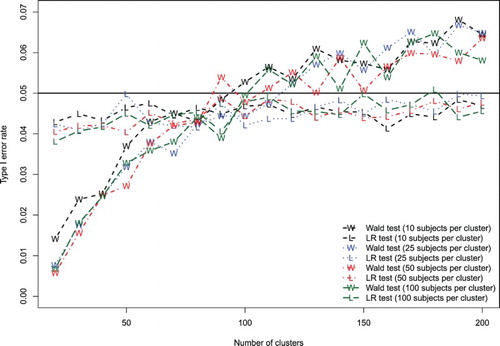
The empirical type I error rates are summarized in Figure 1. We have superimposed on this figure a horizontal line denoting the nominal type I error rate of 0.05. The likelihood ratio test tended to be slightly conservative, with empirical type I error rates that ranged between 0.038 and 0.051. The empirical type I error rate of the likelihood ratio test increased marginally, approaching the nominal type I error rate, with increasing number of clusters. In contrast to this, the Wald test was very conservative when the number of clusters was low (empirical type I error rates of less than 0.02 when there were only 20 clusters). The empirical type I error rate of the Wald test increased substantially with increasing number of clusters. When the number of clusters was large (N_cluster above 150), the null hypothesis was rejected in more than 6% of the samples. The number of subjects per cluster had no discernible impact on the empirical type I error rate of either test.

Figure 1. Effect of number of clusters on Type I error rate (linear model).

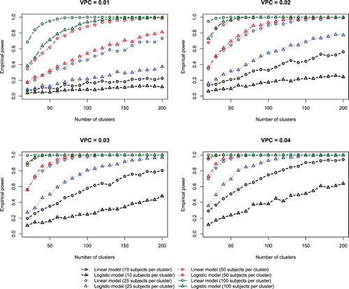
The empirical estimates of statistical power are reported in Figure 2. There is one panel for each of the 10 non-null values of the VPC. For a given value of the VPC, statistical power increased with both an increasing number of clusters and with an increasing number of subjects per cluster. When the magnitude of the effect of clustering was very weak (VPC = 0.01 or 0.02), then, for a given number of clusters, the effect of the number of subjects per cluster on statistical power was dramatic. For example, when the VPC was equal to 0.01, the statistical power was approximately 20% when there were 200 clusters with 10 subjects per cluster, whereas statistical power exceeded 90% when there were 50 or 100 subjects per cluster. When the magnitude of the effect of cluster was much stronger (VPC = 0.10), a low number of clusters (e.g. 20) combined with a low number of subjects per cluster (e.g. 10) still resulted in suboptimal statistical power (< 80% power). Finally, for any given combination of conditions the likelihood ratio test tended to have modestly greater statistical power than did the Wald test.

Figure 2. Effect of number of clusters on power to detect a non-zero variance (linear model).

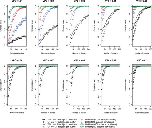
Figure 3. Effect of number of clusters on Type I error rate (logistic model).

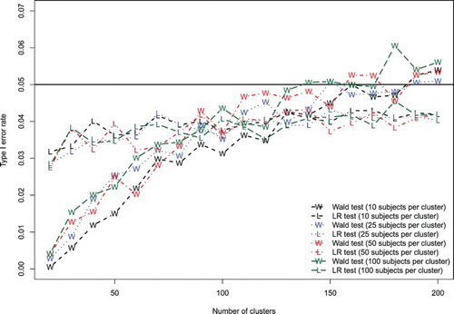
Figure 4. Effect of number of clusters on power to detect a non-zero variance (logistic model).

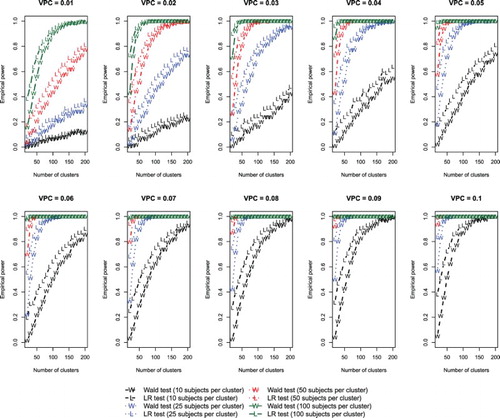
Figure 5. Comparison of LRT type I error rate: linear vs. logistic models.

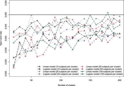
Figure 6. Comparison of LRT power for linear vs. logistic model.

3.2.2. Logistic random effects model

The results for the logistic random effects model are summarized in Figure 3 (empirical type I error rate) and Figure 4 (empirical estimates of statistical power). Patterns similar to those observed for the linear random effects model were observed.

We explored some differences between the empirical type I error rates for the linear model and the logistic model. Given the preceding results showing that the likelihood ratio test was superior to the Wald test, we restricted this comparison to empirical type I error rates for the likelihood ratio test.

In Figure 5, we compare the empirical type I error rates for the likelihood ratio tests for the linear and logistic random effects model. While the likelihood ratio test was conservative for both models, we observed that for a given number of clusters and a given number of subjects per cluster, the empirical type I error rate for the logistic model was lower than that for the linear model. The likelihood ratio test for the linear model had empirical type I error rates closer to the nominal level than did the likelihood ratio test for the logistic model.

In Figure 6, we compare estimates of empirical statistical power when using the likelihood ratio test with the linear model and the logistic model for the four lowest values of the VPC (0.01, 0.02, 0.03, and 0.04). We observed that for a given VPC, number of clusters, and number of subjects per cluster, the likelihood ratio test applied to a linear model had greater statistical power than did the likelihood ratio test applied to a logistic model.

4. Discussion

We conducted an extensive set of Monte Carlo simulations to examine the effect of the number of clusters and the number of subjects per cluster on the statistical power to detect a non-zero variance of the distribution of the random effects. We also compared the empirical type I error rate of the Wald test with that of the likelihood ratio test. We examined both the linear random effects model for use with continuous outcomes and the logistic random effects model for binary outcomes. We found that statistical power increased with both an increasing number of clusters and an increasing number of subjects per cluster. When the random effects variance was very low (VPCs of 0.05 or smaller), increasing the number of subjects per cluster had a substantial effect on power. The likelihood ratio test was slightly conservative, with empirical type I error rates that ranged between 0.038 and 0.051 for the linear random effects model over the range of conditions we explored. The Wald test had very low empirical type I error rates when the number of clusters was low (50 or below), and type I error rates that exceeded 0.05 when the number of clusters was large (150 or above).

Our finding that the statistical power increases with an increasing number of clusters is not surprising. Intuitively, as the number of clusters increases, one is able to estimate the between-cluster variation in outcomes more precisely, implicitly leading to increased power. It is less obvious that statistical power would increase with the number of subjects per cluster. However, intuitively, as the number of subjects per cluster increases, the cluster random intercepts are estimated more precisely and so their variance, in turn, is also estimated more precisely.

As noted in the Introduction, Molenberghs and Verbeke noted that while the likelihood ratio test and the Wald test are asymptotically equivalent, the former is easier to implement and should be considered the default [4]. However, they suggested that additional evaluations and simulations were necessary in order to evaluate the performance of these tests in small samples (p.27). The simulations provided in the current study address this void identified by Molenberghs and Verbeke. While these two tests are asymptotically equivalent, we have shown that they perform differently from one another when the number of clusters is less than or equal to 200 and the number of subjects per cluster is less than or equal to 100. Thus, in settings similar to those encountered by many applied researchers, these two tests should not be viewed as asymptotically equivalent. Instead, the likelihood ratio test should always be preferred.

We examined two different tests for a non-null variance of the random effects distribution. These two tests were selected as they appear to be the most commonly used. In SAS PROC GLIMMIX, the default output includes estimates of the covariance parameters and their asymptotic standard errors (thereby allowing the construction of a Wald test). We note that the mixed and melogit multilevel linear and logistic regression commands in Stata automatically report the results of the likelihood ratio test comparing the fitted model to its constrained counterpart and so the reader does not need to manually fit the constrained model each time. We provide SAS code for evaluating the likelihood ratio test for a linear model (Appendix A) and for a logistic regression model (Appendix B).

Fitzmaurice and Lipsitz proposed a permutation test for the variance components in multilevel generalized linear models. In this approach, the estimated variance is compared to the distribution of estimated variances generated when repetitively refitting the model to different versions of the original data where the cluster indices have been randomly permuted [8]. They demonstrated this method had the correct type I error rate under the null hypothesis that the variance is zero. We did not consider this test for three reasons. First, due to the rarity with which it is employed (the article has been cited only 10 times in the non-methodological literature since its publication 10 years ago [Source: Science Citation Index, date accessed: 18 October 2017]). Second, because it is not implemented in standard software for fitting multilevel models. Third (and most importantly), because it would have increased the computational complexity of the simulations by a factor of 200 (since they recommended using 200 permutations of the data to estimate the distribution of the test statistic under the null hypothesis). The current simulations required approximately 237 hours of computer time (approximately 9.9 days). Using 200 resamplings per simulated dataset would increase this by approximately 1975 days. Given that the permutation-based approach is not implemented in several popular statistical software packages, there is value in knowing in which situations the likelihood ratio test performs well.

We observed that the likelihood ratio test was more conservative for the logistic random effects model than it was for the linear random effects model. As noted above, the sampling distribution of the likelihood ratio test statistic under the null hypothesis is $0.5{\chi }_0^2+0.5{\chi }_1^2$ [4]. However, Fitzmaurice et al. suggest that this sampling distribution is only under the linear mixed model, and suggest that the appropriate mixture of chi-square distributions has yet to be derived for the generalized linear mixed model [8,p.945]. If indeed the sampling distribution of the likelihood ratio statistic under the null hypothesis does not follow a $0.5{\chi }_0^2+0.5{\chi }_1^2$distribution, this might explain why the empirical type I error rate for the logistic model is further from the nominal value than it is for the linear model. Similarly, this may explain why, for a given value of the VPC, number of clusters and number of subjects per cluster, statistical power was greater when using the likelihood ratio test with the linear model compared to with the logistic model. Another explanation for the differences in the empirical type I error rates differed between the logistic model and the linear model is the different estimation methods that were used. The linear models were estimated using restricted maximum likelihood estimation, while the logistic models were estimated using maximum likelihood estimation.

Maas and Hox conducted a series of simulations to determine sufficient sample sizes for fitting multilevel linear models [9]. They allowed the number of clusters to take three values (30, 50, and 100), the number of subjects per cluster to take three values (5, 30, and 50), and the intraclass correlation coefficient to take three values (0.1, 0.2, and 0.3). Their focus was on the effects of these factors on the accuracy of estimated regression coefficients and variance components and their associated standard errors. They found that regression coefficients and variance components were estimated without bias. However, the standard errors of the estimated variance components tended to be too small. With 30 clusters, the standard errors were approximately 15% too small. Their paper focused solely on the estimation of regression parameters, while the focus of the current paper was on statistical power. In their paper, Maas and Hox reviewed a series of unpublished manuscripts and conference proceedings that examine issues related to sample size and estimation of multilevel models. These unpublished manuscripts appeared to focus primarily on the estimation of regression parameters. The novel contribution of the current study is its focus on the effect of number of clusters and number of subjects per cluster on statistical power to detect a non-null variance component.

The primary objective of the paper was to examine the effect of the number of clusters and the number of subjects per cluster on the statistical power to detect a non-zero variance component. As a secondary objective, we compared the performance of the Wald test with that of the likelihood ratio test. Our finding that the performance of the Wald test was suboptimal is not novel. Raudenbush and Bryk suggest that the normality approximation of the sampling distribution of the Wald test statistic may be very poor when the random effects variance is close to zero [6,p.64]. A similar caution is echoed by Hox [5,p.47]. While many researchers with experience with multilevel analysis may be aware that the likelihood ratio test is preferable to the Wald test, many applied analysts may be unaware of this. Maas and Hox suggest that the use of the Wald test to test random effects variances is widespread [9]. A novel contribution of the current paper is to examine the performance of the likelihood ratio test in small-sample settings when either the number of clusters or the number of subjects per cluster is small.

In conclusion, both increasing number of clusters and increasing number of subjects per cluster are associated with increased statistical power to detect a non-null variance of the random effects. The likelihood ratio test had greater power than the Wald test. The likelihood ratio test had empirical type I error rates that were slightly conservative. These patterns of results applied to both the linear and logistic regressions, but were more pronounced for the latter. The likelihood ratio test should be used instead of the Wald test for testing whether the variance of the random effects is different from zero.

Acknowledgements

The opinions, results and conclusions reported in this paper are those of the authors and are independent from the funding sources. No endorsement by ICES or the Ontario MOHLTC is intended or should be inferred. Dr Austin is supported in part by a Career Investigator award from the Heart and Stroke Foundation.

Disclosure statement

No potential conflict of interest was reported by the authors.

Additional information

Funding

This study was supported by the Institute for Clinical Evaluative Sciences (ICES), which is funded by an annual grant from the Ontario Ministry of Health and Long-Term Care (MOHLTC). This research was supported by an operating grant from the Canadian Institutes of Health Research (CIHR) [MOP 86508].

Appendix A. SAS code for evaluating the likelihood ratio test for a linear regression model

proc mixed data=cohort;

 /* Linear model with no random effects */

 class cluster_id;

 model y = x;

 ods output FitStatistics = MLinfo1;

run;

data MLinfo1;

 set MLinfo1;

 if Descr = "\,-2 Res Log Likelihood"\;;

 Deviance_LM = Value;

 keep Deviance_LM;

run;

proc mixed data=cohort covtest;

 /* Linear model with random effects */

 class cluster_id;

 model y = x;

 random intercept /subject=cluster_id;

 ods output FitStatistics = MLinfo2;

run;

data MLinfo2;

 set MLinfo2;

 if Descr = "\,-2 Res Log Likelihood"\;;

 Deviance_LMM = Value;

 keep Deviance_LMM;

run;

data results;

 merge MLinfo1 MLinfo2;

 LRT = abs(Deviance_LM - Deviance_LMM);

 pvalue = (1 - probchi(LRT,1))/2;

run;

proc print data=results;

run;

Appendix B. SAS code for evaluating the likelihood ratio test for a logistic regression model

proc logistic data=cohort descending;

 /* Fit logistic regression model with no random effects */

 model y = x;

 ods output FitStatistics = MLinfo1;

run;

data MLinfo1;

 set MLinfo1;

 if Criterion = "\,-2 Log L"\;;

 Deviance_LR = InterceptAndCovariates;

 keep Deviance_LR;

run;

proc glimmix data=cohort method=quad (qpoints=7);

/* Fit logistic regression model with random effects */

 class cluster_id;

 model y = x /dist=binomial;

 random intercept /subject=cluster_id;

 ods output FitStatistics = MLinfo2;

run;

data MLinfo2;

 set MLinfo2;

 if Descr = "\,-2 Log Likelihood"\;;

 Deviance_GLMM = Value;

 keep Deviance_GLMM;

run;

data results;

 merge MLinfo1 MLinfo2;

 LRT = abs(Deviance_LR - Deviance_GLMM);

 pvalue = (1 - probchi(LRT,1))/2;

run;

proc print data=results;

run;

References

- Snijders T, Bosker R. Multilevel analysis: an introduction to basic and advanced multilevel modeling. London: Sage; 2012.
- Goldstein H. Multilevel statistical models. West Sussex: John Wiley & Sons; 2011.
- Goldstein H, Browne W, Rasbash J. Partitioning variation in generalised linear multilevel models. Underst Stat. 2002;1:223–232. doi: 10.1207/S15328031US0104_02
- Molenberghs G, Verbeke G. Likelihood ratio, score, and Wald tests in a constrained parameter space. Am Stat. 2007;61(1):22–27. doi: 10.1198/000313007X171322
- Hox JJ. Multilevel analysis: techniques and applications. New York (NY): Routledge, Taylor & Francis Group; 2010; p. 1–368.
- Raudenbush SW, Bryk AS. Hierarchical linear models: applications and data analysis methods. Thousand Oaks (CA): Sage; 2002.
- Self SG, Liang K-Y. Asymptotic properties of maximum likelihood estimators and likelihood ratio tests under nonstandard conditions. J Am Stat Assoc. 1987;82:605–610. doi: 10.1080/01621459.1987.10478472
- Fitzmaurice GM, Lipsitz SR, Ibrahim JG. A note on permutation tests for variance components in multilevel generalized linear mixed models. Biometrics. 2007;63:942–946. doi:10.1111/j.1541-0420.2007.00775.x.
- Maas CJ, Hox JJ. Sufficient sample sizes for multilevel modeling. Methodology. 2005;1(3):86–92. doi: 10.1027/1614-2241.1.3.86