Bayesian inference for mixtures of von Mises distributions using reversible jump MCMC sampler

Abstract

Circular data are encountered in a variety of fields. A dataset on music listening behaviour throughout the day motivates development of models for multi-modal circular data where the number of modes is not known a priori. To fit a mixture model with an unknown number of modes, the reversible jump Metropolis-Hastings MCMC algorithm is adapted for circular data and presented. The performance of this sampler is investigated in a simulation study. At small-to-medium sample sizes $(n\le 100)$, the number of components is uncertain. At larger sample sizes $(n\ge 500)$ the estimation of the number of components is accurate. Application to the music listening data shows interpretable results that correspond with intuition.

Keywords:

• Markov chain Monte Carlo
• circular statistics
• von Mises
• mixture models

2010 Mathematics Subject Classification:

• 62F15

1. Introduction

Circular data are data that can be represented as angles in two-dimensional space. Examples of measurements that result in circular data include directions on a compass ($0^{\circ }$–${360}^{\circ }$), time of day (0–24 hours) or day of year (0–365 days). These data are encountered across behavioural research [1,2] and many other scientific disciplines.

Analysis of circular data requires special statistical methods due to the periodicity of the sample space. For example, the arithmetic mean of the two time points 00:30h and 23:30h would be 12:00 h, while the circular mean is 00:00 h, which is clearly a preferable central tendency in this case. Several books on circular statistics are available, in particular Pewsey et al. [3], Mardia and Jupp [4], Fisher [5].

This paper will focus on the modelling of multi-modal circular data with mixtures with an unknown number of components. Mixture models often assume the number of mixture components to be known, although this is rarely true in practice. As a solution, the number of mixture components is usually selected by comparing information criteria such as the AIC [6] or BIC [7]. Such an approach allows selection of a mixture model with the best-fitting number of components, but entirely ignores our uncertainty about the parameter determining the number of components.

A more natural and sophisticated approach is to treat the number of modes as unknown, and obtaining the uncertainty around the number of modes jointly with the rest of the analysis. The main contribution of this paper is to provide an algorithm to perform a fully Bayesian mixture model that correctly captures the uncertainty about the number of components, as well as showing its usefulness and interpretability with a real data example.

The motivating example for this paper is a data set on music listening behaviour. The data was provided by music service 22tracks,¹ and consists of the time of day (on the 24-hour clock) at which a user played a particular song. The user is initially presented with a genre of music, which is selected uniformly random over the genres. The aim of our analysis is to determine which genres are listened to most at certain times, so the most relevant genre at a given time can be presented. In addition, a model where parameters can be directly interpreted may allow us to understand what drives music listening behaviour.

The base distribution for our circular mixture model will be the von Mises distribution, which is commonly used for analysis of circular data and can be considered the circular analogue of the Normal distribution. Von Mises mixture models with a fixed number of modes have been developed previously in a frequentist setting [8], for example using the Expectation Maximization (EM) algorithm [9,10]. Beyond fitting, some work has also been done on hypothesis testing for von Mises mixtures [11–13]. Bayesian analysis for this type of model can be performed through Markov chain Monte Carlo (MCMC) sampling [14,15]. In particular, the high-dimensional variant of this mixture model has seen some popularity due to several appealing applications such as text mining, which has led to an R package for this model [16]. Such high-dimensional circular mixtures use the von Mises-Fisher distribution on hyperspheres, with the von Mises as a special case. We will focus on the circular mixture model only.

The core difficulty in employing MCMC samplers in such applications is that the parameter space is of variable dimension. That is, if there are more components in the mixture model, there are more parameters. Therefore, the usual MCMC approaches do not provide a way to explore the whole parameter space, and we must use a solution such as Reversible jump MCMC [17,18]. In a reversible jump MCMC sampler, we allow moves between parameter spaces by use of a special case of the Metropolis-Hastings (MH) acceptance ratio [19]. This paper provides a detailed account of the adaptation of a reversible jump sampler for von Mises mixtures.

Three major contributions are made to the field of mixture modelling for circular data. First, this paper presents the first application of the reversible jump sampler to this setting, which allows us to perform inference on the amount of components in the mixture model. Second, a novel split move, which makes use of the trigonometric properties of the von Mises distribution, allows the sampler to move across the parameter space efficiently. Lastly, a simulation study is performed to show that this method performs well in common research scenarios.

Several alternative approaches for Bayesian modelling of multi-modal circular data could be considered. Most are found in the field of Bayesian non-parametrics, such as Dirichlet process mixture models [20], the Generalized von Mises distribution [21], log-spline distributions [22] or a family of densities based on non-negative trigonometric sums [23]. Such approaches generally have the advantage of making fewer assumptions about the distribution of the data. However, none of these methods provide a way for direct inference on the number of subpopulations (ie. components) making up the mixture, and the parameters in the mixture model with unknown number of components are much more interpretable.

Therefore, the approach taken in this paper can be seen as a useful in-between step between mixture models with a fixed number of components and non-parametric approaches. Compared to fixed-component mixture models, our approach is more realistic in the uncertainty about the amount of components, allows performing inference about the number of components, but also enables leaving the number of components to be uncertain. In particular, while information criteria based methods also allow selection of the most likely number of components, our approach provides a posterior probability distribution around the number of components, and as such acknowledges that the selected number of components can be wrong. Compared to non-parametric approaches, our approach features much more interpretable parameters and inference, at the cost of taking more assumptions about the shape of the distribution. Concluding, if the number of components is known or not of interest, a fixed-component mixture model can be preferred for simplicity, while if density estimation is the goal a fully non-parametric approach may be the best choice. If the number of components is not known, of interest, and interpretation of the parameters of subpopulations is of interest, our method aligns the best with these goals.

The paper is organized as follows. Section 2 describes the model and chosen priors. Section 3 contains the description and implementation of each of the steps involved in sampling the model parameters. In Section 4 the performance of the sampler is investigated in a simulation study. The sampler is applied to the 22tracks data in Section 5. Finally, the results are discussed in Section 6.

2. Von Mises mixture model

In this section, the von Mises-based mixture model will be developed. First, its general form will be given. Second, the likelihoods necessary for inference are discussed. Third, priors for this model are shortly discussed.

2.1. Von Mises mixture density

The von Mises distribution is a symmetric, unimodal distribution commonly used in the analysis of circular data. Its density is given by (1) $f_{VM}(\theta \mid \mu ,\kappa )=\frac{1}{2\pi I_0(\kappa )}\exp (\kappa \cos (\theta -\mu )),$(1) where $\theta \in [0,2\pi )$ is an angle measured in radians, $\mu \in [0,2\pi )$ is the mean direction, $\kappa \in [0,\mathrm{\infty })$ is a non-negative concentration parameter and $I_0(\cdot )$ is the modified Bessel function of the first kind and order zero.

When data consist of observations from multiple subpopulations for which the labels are not observed, the distribution of the pooled observations can be described by a mixture model. For example, times at which people listen to music are expected to coincide with daily events, such as dinner time or the daily commute, which are clustered around certain time points that show up as modes in the data set.

The density of the pooled observations can be expressed as a mixture (2) $f(\theta \mid \mathit{w},\mathit{\mu },\mathit{\kappa })=\sum _{j=1}^g{w}_j{f}_{VM}(\theta \mid {\mu }_j,{\kappa }_j),$(2) where $g\in {\mathbb{Z}}_{+}$ is the number of components in the mixture, $\mathit{\mu }=({\mu }_1,\dots ,{\mu }_g)$ and $\mathit{\kappa }=({\kappa }_1,\dots ,{\kappa }_g)$ are vectors of distribution parameters of each von Mises component and a vector $\mathit{w}=(w_1,\dots ,w_g)$ containing the relative size of each component in the total sample, called the weight vector. Weights, which are also sometimes called mixing probabilities, satisfy the usual constraints to lie on the simplex, that is $0\le w_j\le 1$ and $\sum _{j=1}^g{w}_j=1$.

2.2. Likelihood

For a dataset $\mathit{\theta }=({\theta }_1,\dots ,{\theta }_N)$ of i.i.d. observations from a mixture of von Mises components, the likelihood is (3) $\mathcal{L}(\mathit{w},\mathit{\mu },\mathit{\kappa },g\mid \mathit{\theta })=\prod _{i=1}^N\sum _{j=1}^g{w}_j{f}_{VM}({\theta }_i\mid {\mu }_j,{\kappa }_j),$(3) where it should be noted that the number of components g is treated as an unknown parameter instead of fixed, and that the lengths of $\mathit{\mu },\mathit{\kappa }$ and $\mathit{w}$ depend on g.

In order to perform inference on ($\mathit{w}$, $\mathit{\mu }$, $\mathit{\kappa }$, g), it will be convenient to include an additional latent vector $\mathit{z}=(z_1,\dots ,z_N)$ that encodes the component to which an observation in $\mathit{\theta }$ is currently attributed. The probability of being attributed to component j is given by $P(z_i=j\mid \mathit{w})=w_j,(i=1,\dots ,N;j=1,\dots ,g).$ The reason for introducing this parameter vector is that conditional on $z_i$, ${\theta }_i$ is an independent observation from its respective component j. That is, $p({\theta }_i\mid z_i=j,{\mu }_j,{\kappa }_j)=f_{VM}({\theta }_i\mid {\mu }_j,{\kappa }_j),$ where inference for ${\mu }_j$ and ${\kappa }_j$ is markedly easier than in the mixture likelihood in Equation (3(3) $\mathcal{L}(\mathit{w},\mathit{\mu },\mathit{\kappa },g\mid \mathit{\theta })=\prod _{i=1}^N\sum _{j=1}^g{w}_j{f}_{VM}({\theta }_i\mid {\mu }_j,{\kappa }_j),$(3) ), because the problem reduces to inference for a single von Mises component. The vector $\mathit{z}$ is called the allocation vector and will be updated as part of the MCMC procedure. Conditional on the allocation vector, the expression for the likelihood of the component parameters $\mathit{\mu },\mathit{\kappa }$ is simply $\mathcal{L}(\mathit{\mu },\mathit{\kappa }\mid \mathit{\theta },\mathit{z})=\prod _{i=1}^N{f}_{VM}({\theta }_i\mid {\mu }_{z_i},{\kappa }_{z_i}).$ As per usual in the Bayesian framework, inference will be performed on the posterior distribution, which is given by (4) $p(\mathit{w},\mathit{\mu },\mathit{\kappa },\mathit{z}\mid \mathit{\theta },g)\propto p(\mathit{w},\mathit{\mu },\mathit{\kappa },\mathit{z},g)\mathcal{L}(\mathit{w},\mathit{\mu },\mathit{\kappa },g\mid \mathit{\theta }),$(4) where the prior $p(\mathit{w},\mathit{\mu },\mathit{\kappa },\mathit{z},g)$ will be discussed next.

2.3. Prior distributions

Although informative priors could be used in practice, it may be difficult to do so for mixture models with an unknown number of components. That is, not knowing whether a component exists makes it unlikely that there is prior information about this component. However, one situation in which there is prior information is when all components are known to lie close to a certain angle. In that case the algorithm can easily be adapted, but we will focus on uninformative priors for simplicity. We will prioritize priors based on their mathematical and computational simplicity. The joint prior $p(\mathit{w},\mathit{\mu },\mathit{\kappa },g)$ is assumed to factor into several independent priors, which will be discussed in turn.

For the von Mises parameters ${\mu }_j$ and ${\kappa }_j$, a conjugate prior [24,25] is used. In principle, one can quite simply include prior information in the hyperparameters of this conjugate prior. However, for the reasons given above, we will focus on uninformative prior hyperparameters. For ${\mu }_j$, this is the circular uniform distribution, which we will write as $p({\mu }_j)\sim \mathcal{U}(0,2\pi ),$ where $\mathcal{U}(a,b)$ is the uniform distribution from a to b.

For ${\kappa }_j$ this is a constant prior $p({\kappa }_j)\propto 1$. Both priors represent a lack of knowledge about these parameters. A more informative prior for ${\kappa }_j$ can also be set in the conjugate prior, for example if highly concentrated von Mises distributions are not expected to represent real subpopulations.

The conjugate prior for $\mathit{w}$ is the Dirichlet distribution. We will use the uninformative $p(\mathit{w})=\mathcal{D}(1,1,\dots ,1),$ which assigns equal probability to all combinations of weights.

The prior for the number of components g is chosen as $p(g)\propto 0.05(1-0.05{)}^{gN}$. This can be seen to be the geometric distribution raised to the power N, the number of observations, used here as a method for penalizing complexity. While somewhat of a pragmatic choice, this prior performs well in practice. The prior prevents overfitting and can be interpreted as the belief that a parsimonious model is preferred, irrespective of the number of observations.

3. Reversible jump MCMC for von Mises mixtures

Bayesian inference for the von Mises mixture model will proceed by sampling from the posterior in Equation (4(4) $p(\mathit{w},\mathit{\mu },\mathit{\kappa },\mathit{z}\mid \mathit{\theta },g)\propto p(\mathit{w},\mathit{\mu },\mathit{\kappa },\mathit{z},g)\mathcal{L}(\mathit{w},\mathit{\mu },\mathit{\kappa },g\mid \mathit{\theta }),$(4) ) using MCMC sampling. As mentioned, standard MCMC will not be able to deal with the changing dimensionality in the parameter space after g changes, and therefore we will resort to reversible jump MCMC to solve this issue.

The reversible jump MCMC algorithm consists of five move types. These moves can be divided into fixed-dimension move types and dimension changing move types. The fixed-dimension moves are the standard moves for MCMC on mixture models. They do not change the component count g and thus do not alter the dimensionality of the parameter space. These moves are

1. updating the weights $\mathit{w}$;

2. updating component parameters ($\mathit{\mu }$, $\mathit{\kappa }$);

3. updating the allocation $\mathit{z}$.

When g is known for a mixture of von Mises components, a sampler consisting of just these three moves would be sufficient.

In many cases however, g is not known and should be estimated as part of the MCMC procedure. This can be achieved by including two more move types, which are the reversible jump move types. They are

1. splitting a component in two, or combining two components;

2. the birth or death of an empty component.

Both of these move types change g by 1 and update the other parameters ($\mathit{w}$, $\mathit{\mu }$, $\mathit{\kappa }$, $\mathit{z}$) accordingly. In our implementation, the move types 1–5 are performed in order. One complete pass over each of these moves will be called an iteration and is the time step of the algorithm. The chosen implementations of these move types will be discussed in detail in the following sections.

3.1. Updating the weights w

Weights $\mathit{w}$ can be drawn directly from their full conditional distribution $p(\mathit{w}\mid \mathit{\mu },\mathit{\kappa },\mathit{z},g)$, which is Dirichlet and dependent only on the current allocation $\mathit{z}$. It is given by $\mathit{w}\mid \mathit{z}\sim \mathcal{D}(n_1+1,\dots ,n_g+1),$ where $n_j$ is the number of observations allocated to component j, given by $n_j=\sum _{i=1}^N{\mathbf{1}}_{z_i=j},$ where $\mathbf{1}$ is an indicator function.

3.2. Updating component parameters μ and κ

The conditional posterior distribution of each ${\mu }_j$ is von Mises and given by (5) ${\mu }_j\mid {\kappa }_j,{\mathit{\theta }}_j\sim VM({\overline{\theta }}_j,R_j{\kappa }_j),$(5) where ${\mathit{\theta }}_j$ is the vector of observations currently allocated to component j and ${\overline{\theta }}_j$ and $R_j$ are respectively the mean direction and the resultant length of ${\mathit{\theta }}_j$.

The conditional distribution of ${\kappa }_j$ can be expressed as $f({\kappa }_j\mid {\mu }_j,{\mathit{\theta }}_j)\propto {I_0({\kappa }_j)}^{-n_j}\exp \{R_j{\kappa }_j\cos ({\mu }_j-\overline{\theta })\}.$ It is not straightforward to sample from this distribution. The method proposed by Forbes and Mardia [26] is applied, which uses a rejection sampler to produce a sample from the full conditional distribution.

3.3. Updating the allocation z

Allocation $z_i$ for each observation is sampled based on the relative densities of the components. For observation i this is given by $P(z_i=j\mid {\theta }_i,\mathit{w},\mathit{\mu },\mathit{\kappa })=\frac{w_j{f}_{VM}({\theta }_i\mid {\mu }_j,{\kappa }_j)}{\sum _{h=1}^g{w}_h{f}_{VM}({\theta }_i\mid {\mu }_h,{\kappa }_h)}.$ This is the categorical (sometimes called 'multinouilli') distribution, and is simple to sample from.

3.4. Dimensionality changing moves

For the dimensionality changing moves we make use of reversible jump moves which are a special case of a Metropolis-Hastings step [18]. The goal is to allow the sampler to move from a current state, which we'll denote by $x=(\mathit{w},\mathit{\mu },\mathit{\kappa },\mathit{z})$, to another state $x^{\prime },$ which has a different size than x. In order to move around the parameter space efficiently, it will be useful to develop several different move types, each moving in a different manner.

In general, each move is implemented by sampling a random vector $\mathit{u}$ that is independent of x, the current state of the sampler. The proposal for a new state $x^{\prime }$ can then be expressed as an invertible function $x^{\prime }(x,\mathit{u})$, to be chosen later, which maps x and u jointly to a proposal $x^{\prime }$. It is required that the move is designed as a pair, such that there also exists the reverse function $x(x^{\prime },\mathit{u})$, which is why the algorithm is called reversible jump. Essentially, we develop a bridge between two spaces of different dimensions, and as a result are able to change the dimensionality.

Given a random vector u and the invertible function $x^{\prime }(x,\mathit{u})$, we can accept or reject the proposal $x^{\prime }$ using a Metropolis-Hastings (MH) acceptance ratio, which can be written as (6) $min\{1,\frac{p(x^{\prime }|y)}{p(x|y)}\frac{r_m(x^{\prime })}{r_m(x)q(\mathit{u})}\left|\frac{\mathrm{\partial }{x}^{\prime }}{\mathrm{\partial }(x,\mathit{u})}\right|\},$(6) where $p(x^{\prime }\mid y)/p(x\mid y)$ is the ordinary ratio of posterior probability of states x and $x^{\prime }$, $r_m(x)$ is the probabilty of choosing move type m from state x, and $q(\mathit{u})$ is the density function of $\mathit{u}$, and the final term $|\mathrm{\partial }{x}^{\prime }/\mathrm{\partial }(x,\mathit{u})|$ is the Jacobian that arises from the change of parameter space from (x, $\mathit{u}$) to $x^{\prime }$. This Jacobian corrects for each state x lying in a space of different dimensionality, and will be 1 if the dimensionality does not change.

The reversible jump moves will dictate how to sample proposals for a new state $x^{\prime }$ given a vector $\mathit{u}$, after which the proposal is accepted or rejected based on the MH ratio just described. The precise form of this MH ratio depends on the move type and the chosen function $x^{\prime }(x,\mathit{u})$. Developing the move types and their associated invertible functions represents a large chunk of the work involved in implementing the reversible jump algorithm for a specific model. Next, some sensible choices for the von Mises model will be discussed.

3.4.1. Split or combine move

The split or combine move is designed as a reversible pair, as is required in the reversible jump framework. That is, any proposed split move is associated with a combine move that would undo it. A split move takes one component and replaces it with two new components. Conversely, a combine move joins two existing components into a single component.

Constructing split/combine proposals for reversible jump MCMC samplers can be done using moment matching [27], where the moments of a combined component are defined to be the sum of the moments of the split components. In the case of von Mises components, the second (linear) moment of a von Mises distribution ignores the circular geometry of this problem, and is mathematically intractable. Rather, its trigonometric moments should be used. The first trigonometric moments of a von Mises component with parameters μ and κ are given by $\alpha =E[\cos (\theta )]=\rho \cos (\mu )$ and $\beta =E[\sin (\theta )]=\rho \sin (\mu )$, where the mean resultant length is $\rho =A(\kappa )=I_1(\kappa )/I_0(\kappa )$ and $A(\kappa )$ can be approximated [4, p. 40].

To make sure that the trigonometric moments represent a valid von Mises distributions, the point described by $(\alpha ,\beta )$ must lie on the unit disc, such that (7) $\sqrt{{\alpha }^2+{\beta }^2}\le 1.$(7) This is important for the reversible jump algorithm, because whenever any dimensionality changing move occurs, any new component must also satisfy these constraints.

The constraint of mapping to valid von Mises components, along with the reversibility condition, limit the set of possible moves. However, any move that follows these limitations will be valid in the sense that it will correctly sample from the desired posterior. As long as the limitations are met, we are free to select move types based on computational efficiency, for example. Computational efficiency will be attained when the proposals are likely to be accepted, which in turn is more likely when the proposals are in some sense 'close' to the original components. This will lead the specific choices for the combine and split moves, which will be discussed next.

Combine move

In the combine move, two current components, say $j_1$ and $j_2$, are combined into a single new component $j^{\ast }$. The combine move can be obtained from a simple weighted sum of the trigonometric moments. That is, the new combined component has trigonometric moments that are a weighted average between the two components that it stems from.

The parameters of the new component are defined by their trigonometric moments and component weight, $(w_{j^{\ast }},{\alpha }_{j^{\ast }},{\beta }_{j^{\ast }})$, by computing (8) $\begin{array}{rl}{w}_{j^{\ast }}& =w_{j_1}+w_{j_2},\\ w_{j^{\ast }}{\alpha }_{j^{\ast }}& =w_{j_1}{\alpha }_{j_1}+w_{j_2}{\alpha }_{j_2},\\ w_{j^{\ast }}{\beta }_{j^{\ast }}& =w_{j_1}{\beta }_{j_1}+w_{j_2}{\beta }_{j_2}.\end{array}$(8) It can be shown that the $(w_{j^{\ast }},{\alpha }_{j^{\ast }},{\beta }_{j^{\ast }})$ correspond to a valid von Mises distribution and weight, due to the convexity of the unit disc (for ${\alpha }_{j^{\ast }},{\beta }_{j^{\ast }}$) and the convexity of the unit interval for the weight $w_{j^{\ast }}$.

Split move

In the split move, we start from joint component $j^{\ast }$ and split it into two components, $j^1$ and $j^2$. The split move must also conform to (8(8) $\begin{array}{rl}{w}_{j^{\ast }}& =w_{j_1}+w_{j_2},\\ w_{j^{\ast }}{\alpha }_{j^{\ast }}& =w_{j_1}{\alpha }_{j_1}+w_{j_2}{\alpha }_{j_2},\\ w_{j^{\ast }}{\beta }_{j^{\ast }}& =w_{j_1}{\beta }_{j_1}+w_{j_2}{\beta }_{j_2}.\end{array}$(8) ) to fulfill the requirement of reversibility, but we must be more careful than in the combine move to prevent the trigonometric moments falling outside the allowed range. We will solve this by proposing the split components from the largest possible disc that is centred at the trigonometric moments of $j^{\ast }$, while being covered by the unit disc. This last property ensures that all proposals are valid.

Next we will discuss how exactly we draw the proposals from within this disc. We can do this by drawing vector $\mathit{u}$ from $u_1\sim \mathcal{U}(0,0.5)u_2\sim \mathcal{U}(0,2\pi )u_3\sim \mathrm{Beta}(2,1),$ where $\mathrm{Beta}(a,b)$ is the Beta distribution, where we have chosen a = 2 and b = 1 to more often select proposals close to the current joint component $j^{\ast }$. Different distributions could be selected here to tune the performance of the method, but these have worked sufficiently in practice.

After drawing the vector $\mathit{u}$, we can obtain our split components by computing (9) $\begin{array}{rl}{\rho }_{max}& =u_3(1-{\rho }_{j^{\ast }})\\ w_{j_1}& =w_{j^{\ast }}{u}_1\\ {\alpha }_{j_1}& ={\alpha }_{j^{\ast }}+\cos (\varphi ){\rho }_{max}\\ {\beta }_{j_1}& ={\beta }_{j^{\ast }}+\sin (\varphi ){\rho }_{max}\end{array}\begin{array}{rl}\varphi & =u_2+\mathrm{atan}2(-{\beta }_{j^{\ast }},-{\alpha }_{j^{\ast }})\\ w_{j_2}& =w_{j^{\ast }}(1-u_1)\\ {\alpha }_{j_2}& ={\alpha }_{j^{\ast }}-\cos (\varphi ){\rho }_{max}{w}_{j_1}/w_{j_2}\\ {\beta }_{j_2}& ={\beta }_{j^{\ast }}-\sin (\varphi ){\rho }_{max}{w}_{j_1}/w_{j_2}.\end{array}$(9) As discussed, different choices are possible, but these were found to perform well in practice. To aid understanding, this procedure is given a visual representation in Figure 1, which will be discussed step by step next.

Figure 1. Construction of split proposal. In Step 1, the green vector shows the current mean resultant vector for the von Mises component to be split. In Step 2, the first split component is placed within the grey disc, by moving $u_3(1-{\rho }_{j^{\ast }})$ in direction $u_2$. Step 3 shows that the second split component (in blue) follows from a combination of trigonometric moments. (a) Step 1. (b) Step 2 and (b) Step 3.

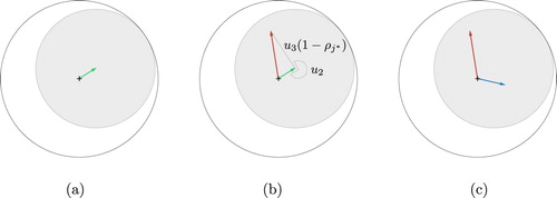
In step 1 (Figure 1(a), the von Mises component $j^{\ast }$ is represented by its trigonometric moments ${\alpha }_{j^{\ast }}$ and ${\beta }_{j^{\ast }}$ as an arrow. The two new components' trigonometric moments must fall inside the unit circle, as to satisfy constraint (7(7) $\sqrt{{\alpha }^2+{\beta }^2}\le 1.$(7) ). To do this, a disc with radius $1-{\rho }_{j^{\ast }}$ centred at $({\alpha }_{j^{\ast }},{\beta }_{j^{\ast }})$ is indicated in grey in the figure, from which the split components will be sampled.

In step 2 (Figure 1(b)), the first new von Mises component $j_1$ is placed relative to the original component. The random direction $u_2$ is rotated so that $\varphi =u_2+\mathrm{atan}2({\beta }_{j^{\ast }},{\alpha }_{j^{\ast }})$ determines the direction in which we will step to obtain a new trigonometric moment of $j_1$. The trigonometric moments of the proposal $({\alpha }_{j_1},{\beta }_{j_1})$ are then computed, in direction φ and a distance of $u_3(1-{\rho }_{j^{\ast }})$ away from $({\alpha }_{j^{\ast }},{\beta }_{j^{\ast }})$.

Step 3 (Figure 1(c)) places the second new von Mises component. Given the original component $j^{\ast }$ and the first new component $j_1$, the moments for the second component $j_2$ are placed. They are found in the opposite direction from $({\alpha }_{j^{\ast }},{\beta }_{j^{\ast }})$, that is $u_2+\pi$. The distance is determined depending on the ratio of the two weights. This can be computed as given in (8(8) $\begin{array}{rl}{w}_{j^{\ast }}& =w_{j_1}+w_{j_2},\\ w_{j^{\ast }}{\alpha }_{j^{\ast }}& =w_{j_1}{\alpha }_{j_1}+w_{j_2}{\alpha }_{j_2},\\ w_{j^{\ast }}{\beta }_{j^{\ast }}& =w_{j_1}{\beta }_{j_1}+w_{j_2}{\beta }_{j_2}.\end{array}$(8) ).

The probability of performing a split move as opposed to a combine move $r_m(x)$ is set to $\frac{1}{2}$, independent of the current state of the MCMC sampler. It then follows that the probability of the corresponding combine move $r_m(x^{\prime })=1-r_m(x)=\frac{1}{2}$ and their ratio $r_m(x^{\prime })/r_m(x)=1$. This can result in an attempted combine move when g = 1, which is immediately rejected.

The Jacobian for the split move is straightforward to derive, but long in form and given by $\begin{array}{rl}\left|\frac{\mathrm{\partial }{x}^{\prime }}{\mathrm{\partial }(x,u)}\right|& =\frac{({\rho }_{j^{\ast }}-1{)}^2{\rho }_{j^{\ast }}{w}_{j^{\ast }}(1-2u_1{)}^2{u}_3}{u_1-1}\\ & \times {(2({\rho }_{j^{\ast }}-1){\rho }_{j^{\ast }}\cos (u_2)u_3+(1-2{\rho }_{j^{\ast }})u_3^2+{\rho }_{j^{\ast }}^2(1+u_3^2))}^{-1/2}\\ & \times [(1-2{\rho }_{j^{\ast }})u_1^2{u}_3^2+{\rho }_{j^{\ast }}^2(1-2u_1+u_1^2(1+u_3^2))\\ & -2({\rho }_{j^{\ast }}-1){\rho }_{j^{\ast }}\cos (u_2)(u_1-1)u_1{u}_3{]}^{-1/2}.\end{array}$ The inverse of this Jacobian is used for the combine move.

3.4.2. Birth or death move

A birth move introduces a new component into the mixture, without assigning any observations to this component. Its inverse, a death move, removes a component that has no observations.

The proposal for a birth move consists of drawing parameters $(w_{j^{\ast }}$, ${\mu }_{j^{\ast }}$, ${\kappa }_{j^{\ast }})$ for a new component. They are chosen from a proposal distribution as $w_{j^{\ast }}\sim \mathcal{U}(0,1){\mu }_{j^{\ast }}\sim \mathcal{U}(0,2\pi ){\kappa }_{j^{\ast }}\sim {\chi }_{10}^2.$ These parameters are then used to construct vector $\mathit{u}=(w_{j^{\ast }}$, ${\mu }_{j^{\ast }}$, ${\kappa }_{j^{\ast }})$. The weights of the other components need to be rescaled such that the sum of weights remains 1. The new weights are $w_j^{\prime }=w_j(1-w_{j^{\ast }})$, for $j\in \{1,\dots ,g\}$.

Notably, as no observations are allocated to the newly created component, the likelihood of the data is unaltered by the move. Additionally, as with the split or combine move type, the probability of performing a birth move $r_m(x)$ is set equal to the probability of performing the corresponding death move $r_m(x^{\prime })$, independent of the state of the MCMC sampler. Therefore, the acceptance probability (6(6) $min\{1,\frac{p(x^{\prime }|y)}{p(x|y)}\frac{r_m(x^{\prime })}{r_m(x)q(\mathit{u})}\left|\frac{\mathrm{\partial }{x}^{\prime }}{\mathrm{\partial }(x,\mathit{u})}\right|\},$(6) ) can be simplified to $min\{1,\frac{p(x^{\prime })}{p(x)}\frac{1}{q(u)}\left|\frac{\mathrm{\partial }{x}^{\prime }}{\mathrm{\partial }(x,u)}\right|\}.$ The Jacobian for a birth move is given by $\left|\frac{\mathrm{\partial }{x}^{\prime }}{\mathrm{\partial }(x,u)}\right|=(1-w_{j^{\ast }}{)}^g.$ For a death move, vector $\mathit{u}$ is given by the component parameters of the component that is removed $j^{\ast }$, $\mathit{u}=(w_{j^{\ast }},{\mu }_{j^{\ast }},{\kappa }_{j^{\ast }})$. Its MH acceptance ratio is the inverse of the MH acceptance ratio of the corresponding birth move.

3.5. Label switching

When fitting a mixture model with a fixed number of components g, label switching [28] can occur when, for example, the means of two components are close and by random chance switch order. This can also be seen as an identifiability problem. When applying a sampler that can jump between parameter spaces and change the number of components as part of the MCMC chain, label switching is very likely to occur, regardless of the distance between means, because split moves do not define an order for the created components.

A simple method of dealing with label switching is by imposing an identifiability constraint, for example by requiring the means to be ordered. This is a crude method that does not work in the case of circular data, since two means will always be ordered the same way on a circle.

A solution is provided by Stephens [29] in the form of a post-processing step to define the most likely allocation of sampled parameters to individual components and does not rely on constraints. The second post-processing algorithm featured in the paper is applied to the samples belonging to each specific g separately.

4. Simulation study

A simulation study was performed to investigate the relative performance of the MCMC sampler in different scenarios. The sampler was implemented in R [30] using the $\mathtt{\text{circular}}$ package [31]. The source code has been made available at https://github.com/pieterjongsma/circular-rjmcmc.

4.1. Simulation scenarios

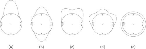
In order to assess the performance in a variety of settings, five true data generating processes were selected to represent either common or particularly difficult mixture datasets to fit. These scenarios are visualized in Figure 2 and consist of (2(a)) a single von Mises component where ${\mu }_1=0$ and ${\kappa }_1=10$, (2(b)) two von Mises components where ${\mu }_1=0$, ${\mu }_2=\pi$ and ${\kappa }_1={\kappa }_2=10$, (2(c)) two von Mises components where ${\mu }_1=-\pi /6$, ${\mu }_2=\pi /6$ and ${\kappa }_1={\kappa }_2=10$, (2(d)) three von Mises components where ${\mu }_1=-\pi /3$, ${\mu }_2=0$, ${\mu }_3=\pi /3$ and ${\kappa }_1={\kappa }_2={\kappa }_3=10$ and (2(e)) a uniform von Mises component ($\kappa =0$). Each scenario is simulated with 50, 100, 250, 500, 1000, 2500 and 10,000 observations across 1000 replications.

Figure 2. Visualization of simulation scenarios used for investigating sampler performance.

4.2. Starting values

The MCMC sampler is initialized with a single component (g = 1) and parameters for the component drawn analogous to a birth move $w=1\mu \sim \mathcal{U}(0,2\pi )\kappa \sim {\chi }_{10}^2.$ The observations are all attributed to this single component by setting the allocation vector as $z_i=1$ for $i\in \{1,\dots ,N\}$.

4.3. Convergence

The convergence of a reversible jump MCMC algorithm is difficult to assess using conventional methods such as the inspection of the sampled values of a parameter. Due to the changing dimensionality, the posterior distributions of individual component parameters depend on the component count g. The chains for these components are expected to jump with every change of g and would therefore not provide a valid measure of convergence. Instead, the likelihood $p(x\mid \mathit{\theta })$ is calculated for each iteration of the MCMC chain for which convergence of the posterior probability is assessed visually. All chains, regardless of starting value and variation in replicated data, converged within a burn-in of 10,000 iterations. After the burn-in, the next 5,000 iterations are retained and used to describe the posterior properties of the simulated dataset.

4.4. Results

For brevity, this section will be focused on the ability of the sampler to recover the number of components g correctly. In addition, performance of model parameters will be assessed for a subset of simulations.

4.4.1. Number of components g

The results for the number of components g of the simulation study are summarized in Table 1. It shows the fraction of replications in which the maximum a posteriori (MAP) estimate of g, $g_{MAP}$, which is the posterior mode, was equal to the simulated g, $g_{TRUE}$. Furthermore, the posterior distribution of g is given, averaged over all replications.

Table 1. Simulation results for each of the scenarios in Figure 2 with sample sizes ranging from n = 50 to n = 10000. Each row represents 1000 replications. The fraction of replications where the estimated g was equal to the simulated g is given under $g_{MAP}=g_{TRUE}$. In addition, the posterior distribution $p(g\mid \theta )$ is given as the average over all replications.

			$p(g\mid \mathit{\theta })$
Scenario	n	$g_{MAP}=g_{TRUE}$	g = 1	g = 2	g = 3	g = 4	$g\ge 5$
2(a)	50	0.40	0.29	0.29	0.21	0.12	0.10
	100	0.73	0.54	0.32	0.11	0.03	0.00
	250	0.88	0.69	0.27	0.04	0.00	0.00
	500	0.94	0.72	0.25	0.03	0.00	0.00
	1000	0.96	0.76	0.22	0.02	0.00	0.00
	2500	0.99	0.82	0.17	0.01	0.00	0.00
	10000	1.00	0.85	0.14	0.01	0.00	0.00
2(b)	50	0.12	0.00	0.10	0.15	0.16	0.59
	100	0.66	0.00	0.50	0.31	0.12	0.06
	250	0.91	0.00	0.81	0.18	0.01	0.00
	500	0.88	0.00	0.77	0.21	0.01	0.00
	1000	0.81	0.00	0.71	0.27	0.02	0.00
	2500	0.71	0.00	0.63	0.34	0.03	0.00
	10000	0.58	0.00	0.54	0.44	0.02	0.00
2(c)	50	0.30	0.05	0.23	0.29	0.21	0.22
	100	0.66	0.08	0.51	0.30	0.09	0.03
	250	0.93	0.03	0.83	0.13	0.01	0.00
	500	0.97	0.01	0.85	0.13	0.01	0.00
	1000	0.98	0.00	0.86	0.13	0.01	0.00
	2500	0.98	0.00	0.89	0.11	0.00	0.00
	10000	1.00	0.00	0.94	0.06	0.00	0.00
2(d)	50	0.30	0.01	0.11	0.22	0.22	0.44
	100	0.60	0.01	0.25	0.45	0.21	0.08
	250	0.84	0.00	0.15	0.78	0.07	0.00
	500	0.96	0.00	0.04	0.91	0.06	0.00
	1000	0.97	0.00	0.02	0.94	0.04	0.00
	2500	0.97	0.00	0.02	0.95	0.03	0.00
	10000	0.98	0.00	0.01	0.98	0.01	0.00
2(e)	50		0.01	0.03	0.05	0.07	0.84
	100		0.15	0.25	0.25	0.17	0.18
	250		0.34	0.37	0.20	0.07	0.02
	500		0.36	0.38	0.19	0.06	0.01
	1000		0.37	0.37	0.19	0.05	0.01
	2500		0.37	0.38	0.19	0.05	0.01
	10000		0.37	0.37	0.21	0.04	0.01

Results with few observations (n = 50) show high uncertainty about the number of components. For these replications, the mode of the posterior distribution for g was rarely equal to the simulated g. As expected, the estimation of g then improves with the number of observations. Most scenarios show a near 100% correct mode $g_{MAP}$ at 1000 observations or more. One exception is scenario 2(b) for n = 10000. Here, g is overestimated and accuracy is seemingly worse than at a smaller sample size. It should be noted that an overestimation of g does not necessarily indicate a problem with the MCMC method. A model with a higher number of components may have a higher likelihood of the data. The chosen prior for g is intended to counter this effect, such that the simpler model is favoured. The prior is seemingly not powerful enough for scenario 2(b) where n = 1000 or larger.

For the uniform scenario 2(e), the column $g_{MAP}=g_{TRUE}$, showing the correspondence between the mode of the posterior distribution and the simulated g, has been omitted. Although this data was simulated as a single component with $\kappa =0$, the interpretation of ‘true’ g of this distribution is ambiguous. For larger datasets, the method favours a small number of components, as expected.

4.4.2. Parameter estimates

Results for the recovery of the von Mises parameters $\mathit{\mu }$ and $\mathit{\kappa }$, are summarized for scenario 2(d) in Table 2. To obtain these estimates, only the MCMC states with three components are retained, so that g = 3 as in the data generating process of scenario 2(d). For each simulated data set, MAP estimates for $\hat{\mathit{\mu }}$ and $\hat{\mathit{\kappa }}$, are computed by estimating the posterior modes from the MCMC sample. Then, these MAP estimates are averaged over all simulated datasets and presented.

Table 2. Parameter estimates for scenario 2(d) with parameters ${\mu }_1=-1.05$, ${\mu }_2=0$, ${\mu }_3=1.05$ and ${\kappa }_1={\kappa }_2={\kappa }_3=10$.

n	${\hat{\mu }}_1$	${\hat{\mu }}_2$	${\hat{\mu }}_3$	${\hat{\kappa }}_1$	${\hat{\kappa }}_2$	${\hat{\kappa }}_3$
50	−0.99	0.01	1.02	183.7	82.0	192.9
100	−1.04	0.00	1.07	161.8	62.6	133.9
250	−1.05	−0.01	1.05	31.6	34.7	17.8
500	−1.05	0.00	1.06	11.9	8.0	10.6
1000	−1.05	0.00	1.05	10.7	8.2	10.5
2500	−1.04	0.01	1.04	10.0	9.7	10.1
10000	−1.04	0.00	1.04	10.0	9.7	10.0

The estimates of component parameters for scenario 2(d) show that in general the method is able to recover the true parameter estimates for μ without bias, even with small sample size (n = 50). The concentration parameter $\mathit{\kappa }$ is overestimated with small samples, but estimates are reasonable for samples where $n\ge 500$. The concentration parameter of the central component, ${\kappa }_2$, is systematically underestimated in this scenario, with ${\kappa }_1$ and ${\kappa }_3$ slightly overestimated except with very large sample sizes. Most likely, the central component is assigned some observations that belong to its two neighbours, and as a result is estimated as less concentrated than the true data generating process.

5. Illustration

As a motivating example, we will apply the reversible jump MCMC sampler to a dataset of listening behaviour, made available by 22tracks. This data will first be described and visualized in Section 5.1. Then, results from applying the sampler to the data are discussed in Section 5.2.

5.1. Dataset

The data provided by 22tracks contain metrics of all users of the service over the span of one week (January 4–10, 2016). The data consist of the time of day (00:00 h to 23:59 h) at which a user played a particular song, categorized by the genre this song was in. In this paper, a subset of the data is used as an illustration. These consist of all observations categorized under one of three genres that were selected arbitrarily. The genres are Indie Electronic, Relax and Deep House. Figure 3 shows kernel density estimates of each genre. It can be seen that depending on the genre, the data features a different number of modes, although determining the precise number of modes is difficult without running the mixture model.

Figure 3. Kernel density estimates of observations for analysed 22tracks genres, using a von Mises kernel with $\kappa =200$. The period of the circle is 24 hours. (a) Indie Electronic (n = 11, 393). (b) Relax (n = 10, 657) and (c) Deep House (n = 4, 757).

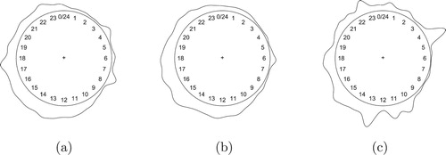
The first goal of this analysis is to estimate the genre that is most likely to be selected at any given time. Supposedly, users listen to the genres available on the 22tracks service at different times of day. For example, Pop might be a genre that users listen to throughout the day while Deep House is preferred during the night. Quantifying this behaviour is valuable for the music service, as it allows them to present the most appropriate genres to users when they visit the site at a particular time.

The second goal is to understand music listening behaviour through the parameters of our mixture components, as the times at which we listen to music are a reflection of life in our society. The mixture components are then interpreted as a subpopulation of observations that correspond to a certain category of music listening, such as listening while working, during transit, or while dancing.

5.2. Results

We apply the mixture model to each genre separately, with starting values as described in Section 4.2, using a burn-in of 10,000 iterations and retaining the next 100,000 iterations for inference. The posterior distributions for component count g are summarized in Table 3. The posteriors are quite different, with the Deep House genre showing a notably higher estimated component count, which is in accordance with the data as displayed in Figure 3.

Table 3. Posterior probability of component counts $p(g)$ for selected 22tracks genres.

	g
Genre	1	2	3	4	5	6	7	8
Indie Electronic	0.01	0.52	0.36	0.10	0.01	0.00	0.00	0.00
Relax	0.00	0.25	0.55	0.18	0.02	0.00	0.00	0.00
Deep House	0.00	0.00	0.00	0.02	0.30	0.37	0.28	0.03

To obtain estimates for the other parameters $\mathit{w}$, $\mathit{\mu }$ and $\mathit{\kappa }$, only the samples for which $g=g_{MAP}$ are used. For Deep House, these are samples where g = 6, for Indie Electronic g = 2 and for Relax g = 3. The parameters have been summarized in Table 4, ordered by the weights $\mathit{w}$.

Table 4. Estimated component parameters for individual genres in 22tracks data. LB and UB indicate the lower and upper bound of the 95% density of the data density of this von Mises component. Components have been ordered according to their respective weights.

					95% density
Genre	j	$\widehat{w_j}$	$\widehat{{\mu }_j}$	$\widehat{{\kappa }_j}$	LB	UB
Indie Electronic	1	0.72	3.73 (14:15 h)	0.89	1.04 (03:58 h)	0.15 (00:33 h)
	2	0.28	5.55 (21:13 h)	0.72	2.77 (10:36 h)	2.05 (07:50 h)
Relax	1	0.54	4.11 (15:43 h)	1.20	1.63 (06:15 h)	0.31 (01:11 h)
	2	0.33	5.49 (20:59 h)	0.85	2.78 (10:37 h)	1.93 (07:22 h)
	3	0.13	3.09 (11:49 h)	1.75	1.10 (04:12 h)	5.09 (19:27 h)
Deep House	1	0.30	3.99 (15:15 h)	2.07	2.25 (08:35 h)	5.74 (21:55 h)
	2	0.28	6.04 (23:04 h)	1.64	3.95 (15:05 h)	1.85 (07:03 h)
	3	0.17	5.13 (19:36 h)	1.59	2.99 (11:27 h)	0.98 (03:45 h)
	4	0.10	2.79 (10:41 h)	33.81	2.45 (09:23 h)	3.13 (11:59 h)
	5	0.08	1.16 (04:27 h)	635.81	1.09 (04:09 h)	1.24 (04:45 h)
	6	0.07	3.40 (12:58 h)	648.16	3.32 (12:41 h)	3.47 (13:16 h)

The Indie Electronic genre shows two broad components spanning most of the day. One is centred at the middle of the day (14:15 h) and one is centred in the evening (21:13 h), most likely corresponding to listening while working and listening at home during the evening. The components have a small concentration, suggesting only slight preference for these times. Such broad components are necessary, because listening occurs throughout the day. Similarly, the Relax genre is given three components with small concentration.

For the Deep House genre, six components provided the best fit. The first three components are broad and similar to the components found for the other genres. The central times are later in the day, as one might expect for this type of music. The sampler was also able to detect and fit the strong concentrations of observations at 10:41, 04:27 and 12:58 h. It is unlikely that these patterns have been created by actual users. More likely, they indicate a special attribute of the data. For example, a computer bot instead of an actual person could have triggered a large amount of plays in a short time span. Although this does not tell us anything about the behaviour of actual users, it is still an interesting property that the sampler detects quite well. In fact, such a component has direct financial implications for this business, as such plays can be rejected to save costs.

Compared to a kernel density model, this provides a much simpler and more interpretable summary of the data. The posterior distribution also provides uncertainty around all of these estimates, although these are not shown here for brevity.

6. Discussion

We have presented a method for Bayesian inference of von Mises mixture distribution. Previous work has assumed the number of components to be known, which is an assumption we have relaxed by employing the reversible jump MCMC algorithm. The main contributions included a novel set of dimensionality changing moves based on the trigonometric properties of the von Mises distribution. In addition, the performance of the method was investigated in a simulation study. Generally, the method performed well. An illustration was provided on music listening behaviour, showing the interpretation of this method.

Results of the simulation study showed that the estimation of the number of components g was accurate for the majority of the simulated sample sizes, so the proposed split and combine moves successfully move between parameter spaces. In one scenario (2(b)), g is overestimated at a very large sample count (n = 10000). In this case the proposed prior for g appears insufficient. A different choice of prior might be able to counter this effect and seems a topic for further investigation. It should be noted that although undesirable, an overfitted mixture is not necessarily problematic in application. The estimation of parameters $\mathit{w}$, $\mathit{\mu }$ and $\mathit{\kappa }$ of the individual components is not directly affected and these parameters remain interpretable. Furthermore, the component weights allow us to gauge the relative importance of each component.

Application to the 22tracks data provides an example for the interpretation of reversible jump MCMC sampler output. It should be noted that the observation counts in the 22tracks data were higher than what showed the most accurate estimation of the simulated component count in the simulation study and as such we did not infer much from the estimated g. Because the parametric von Mises model is easy to interpret, one can compare the results with intuition. The estimated component parameters $\mathit{\mu }$ and $\mathit{\kappa }$ in the provided example seem reasonable as they indicate listening to occur during daytime and in the evening.

In conclusion, the method presented in this paper provide a reversible jump MCMC sampler that is shown to perform well on simulated data as well as a real world example.

Disclosure statement

No potential conflict of interest was reported by the author(s).

ORCID

Kees Mulder  http://orcid.org/0000-0002-5387-3812

Additional information

Funding

This work was supported by a Vidi grant awarded to I. Klugkist from NWO, the Dutch Organization for Scientific Research (NWO 452-12-010).

Notes

1 Unfortunately this music service is now defunct. Previously it was found at http://www.22tracks.com/.

References

- Gurtman MB. Exploring personality with the interpersonal circumplex. Soc Personal Psychol Compass. 2009;3(4):601–619. doi: 10.1111/j.1751-9004.2009.00172.x
- Mechsner F, Kerzel D, Knoblich G, et al. Perceptual basis of bimanual coordination. Nature. 2001;414(6859):69–73. doi: 10.1038/35102060
- Pewsey A, Neuhäuser M, Ruxton GD. Circular statistics in R. Oxford University Press; 2013.
- Mardia KV, Jupp PE. Directional statistics. Wiley; 2000.
- Fisher NI. Statistical analysis of circular data. Cambridge: Cambridge University Press; 1995.
- Akaike H. A new look at the statistical model identification. IEEE Trans Automat Contr. 1974;19(6):716–723. doi: 10.1109/TAC.1974.1100705
- Schwarz G. Estimating the dimension of a model estimating the dimension of a model. Ann Stat. 1978;6(2):461–464. doi: 10.1214/aos/1176344136
- A Mooney J, Helms PJ, Jolliffe IT. Fitting mixtures of von Mises distributions: a case study involving sudden infant death syndrome. Comput Stat Data Anal. 2003;41(3–4):505–513. doi: 10.1016/S0167-9473(02)00181-0
- Banerjee A, Dhillon IS, Ghosh J, et al. Clustering on the Unit Hypersphere using von Mises-Fisher distributions. J Mach Learn Res. 2005;6(Sep):1345–1382.
- McLachlan G, Krishnan T. The EM algorithm and extensions. John Wiley & Sons; 2007.
- Chen J, Li P, Fu Y. Testing homogeneity in a mixture of von Mises distributions with a structural parameter. Canadian J Stat. 2008;36(1):129–142. doi: 10.1002/cjs.5550360112
- Fu Y, Chen J, Li P. Modified likelihood ratio test for homogeneity in a mixture of von Mises distributions. J Stat Plan Inference. 2008;138(3):667–681. doi: 10.1016/j.jspi.2007.01.003
- Paindaveine D, Verdebout T. Inference on the mode of weak directional signals: a Le Cam perspective on hypothesis testing near singularities. Ann Stat. 2017;45(2):800–832. doi: 10.1214/16-AOS1468
- Besag J, Green P, Higdon D, et al Bayesian computation and stochastic systems. Stat Sci. 1995;10(1):3–41. doi: 10.1214/ss/1177010123
- Tierney L. Markov chains for exploring posterior distributions. Ann Stat. 1994;22(4):1701–1728. doi: 10.1214/aos/1176325750
- Hornik K, Grün B. movMF: an R package for fitting mixtures of von Mises-Fisher distributions. J Stat Softw. 2014;58(10):1–31. doi: 10.18637/jss.v058.i10
- Green PJ. Reversible jump Markov chain Monte Carlo computation and Bayesian model determination. Biometrika. 1995;82(4):711–732. doi: 10.1093/biomet/82.4.711
- Richardson S, Green P. On Bayesian analysis of mixtures with unknown number of components. J R Stat Soc Ser B (Stat Methodol). 1997;59(4):731–792. doi: 10.1111/1467-9868.00095
- Hastings WK. Monte Carlo sampling methods using Markov chains and their applications. Biometrika. 1970;57(1):97–109. doi: 10.1093/biomet/57.1.97
- Ghosh K, Jammalamadaka R, Tiwari R. Semiparametric Bayesian techniques for problems in circular data. J Appl Stat. 2003;30(2):145–161. doi: 10.1080/0266476022000023712
- Gatto R, Jammalamadaka R. The generalized von Mises distribution. Stat Methodol. 2007;4(3):341–353. doi: 10.1016/j.stamet.2006.11.003
- Ferreira JTAS, Juárez MA, Steel MFJ. Directional log-spline distributions Directional log-spline distributions. Bayesian Anal. 2008;3(2):297–316. doi: 10.1214/08-BA311
- Fernández-Durán JJ, Mercedes Gregorio-Domínguez M. Bayesian analysis of circular distributions based on non-negative trigonometric sums. J Stat Comput Simul. 2016;86(16):3175–3187. doi: 10.1080/00949655.2016.1153641
- Guttorp P, Lockhart RA. Finding the location of a signal: A Bayesian analysis. J Am Stat Assoc. 1988;83(402):322–330. doi: 10.1080/01621459.1988.10478601
- Mardia KV, El-Atoum S. Bayesian inference for the von Mises-Fisher distribution. Biometrika. 1976;63(1):203–206. doi: 10.1093/biomet/63.1.203
- Forbes PGM, Mardia KV. A fast algorithm for sampling from the posterior of a von Mises distribution. J Stat Comput Simul. 2014;85(13):2693–2701. doi: 10.1080/00949655.2014.928711
- Brooks SP, Giudici P, Roberts GO. Efficient construction of reversible-jump Markov chain Monte Carlo proposal distributions. J R Stat Soc Ser B (Stat Methodol). 2003;65(1):3–55. doi: 10.1111/1467-9868.03711
- Jasra A, Holmes CC, Stephens DA. Markov chain Monte Carlo methods and the label switching problem in Bayesian mixture modeling. Stat Sci. 2005;20(1):50–67. doi: 10.1214/088342305000000016
- Stephens M. Dealing with label switching in mixture models. J R Stat Soc Ser B (Stat Methodol). 2000;62(4):795–809. doi: 10.1111/1467-9868.00265
- R Core Team, R: a language and environment for statistical computing [computer software manual]. Vienna, Austria. Available from: https://www.R-project.org/. 2015.
- Agostinelli C, Lund U. R package circular: circular Statistics (version 0.4-7) [computer software manual]. CA: Department of Environmental Sciences, Informatics and Statistics, Ca' Foscari University, Venice, Italy. UL: Department of Statistics, California Polytechnic State University, San Luis Obispo, California, USA. Available from: https://r-forge.r-project.org/projects/circular/. 2013.