The package: nonparametric regression using local rotation matrices in

ABSTRACT

The package implements nonparametric (smooth) regression for spherical data in , and is freely available from the Comprehensive Archive Network (CRAN), licensed under the MIT License. It can be used for regression when both the response and explanatory variables lie on the unit sphere. The model uses a flexible kernel-type regression determined by a rotation which depends on a smoothing parameter as well as the prediction point. A particular kernel is proposed and a smoothing parameter selection procedure is also provided. Finally, some examples are included in the package.

Keywords:

• Bias reduction
• local smoothing
• non-rigid rotation estimation
• singular value decomposition
• skew-symmetric matrices
• spherical kernels

1. Introduction

Statistical methods for variables that have a spherical nature occur in various fields. There are two main categories of spherical data: directional and shape data. Standard examples of directional phenomena are: directions of winds, marine currents, Earth's main magnetic field and rocket nozzle internal combustion flow. Several recent examples of spherical data – which concern genome sequence representations, text analysis and clustering, morphometrics and computer vision – have been collected by [1]. Shape analysis [2] deals with the similarity between two objects, each being represented by a set of landmarks, after superimposing them by translation, scaling and rotation. A further domain for spherical data is in the field of compositional data analysis, i.e. positive vectors whose components add to a given constant. If the latter is set to 1, a square root transformation puts these data onto the unit hypersphere.

Dependence involving spherical variables has emerged as a very interesting problem. This is the case of multivariate regression where both the explanatory ($\mathit{X}$) and response ($\mathit{Y}$) observations lie on a unit hypersphere, denoted by ${\mathbb{S}}^{d-1},d\ge 2$. For example, in geology, the dependence of one tectonic plate relative to another has been studied in [3]; in crystallography it is of interest to relate an axis of a crystal to an axis of a standard coordinates system [4]; and in the orientation of a satellite it is necessary to study dependence between directions of stars and directions in a terrestrial coordinate system [5]. In machine vision, it is interesting to compare the directions detected by two different sensors. Spherical regression was used in calibration experiments for an electromagnetic motion-tracking system, with the aim of tracking the orientation and position of a sensor moving in three-dimensional space in which the observed orientation is modelled as a rotationally perturbed version of the true one [6].

An obvious application of our methodology is to monitor and predict the movement of the magnetic north pole, which has recently been in the media [7]. The location of magnetic north at time t can be represented by a point on the 3-d sphere, and one might consider an AR-type model of the form ${\hat{\mathit{x}}}_t=f({\mathit{x}}_{t-1})$ with various representations for the function f.

Concerning the parametric framework, spherical–spherical regression has been studied by [8]. According to his model, two variates lying on ${\mathbb{S}}^{d-1}$ are related by an unknown rotation which needed to be estimated. [9] considered the case where the experimental errors follow a von Mises–Fisher distribution with a large concentration parameter and the sample size is fixed. Then, [10] proposed a spherical regression using link functions based on Möbius transformations for the case of an ordinary sphere.

Nonparametric approaches to regression of spherical data have been proposed by [11] (see also the references therein). They used a strategy which is similar to Euclidean smoothing, in which a polynomial is used to locally (splines, wavelets or Taylor-like ones) or globally (spherical harmonics) model the regression function. As a result, they generally work component-wise, when used to predict spherical responses. A serious problem with some of these approaches lies in explicitly modelling (or excluding) any correlation between dimensions, that, due to the spherical geometry, is inherent. On the other hand, it may be noted that those methods which work component-wise do not require $\mathit{x}$ and $\mathit{y}$ to lie on spheres of the same dimension. Recently, [12] propose a very flexible, simple regression model where for each location of the hypersphere a specific rotation matrix is to be estimated. This technique is based on approximations of rotation matrices based on a series expansion and leads to an iterative estimation within a Newton–Raphson learning scheme which exhibits bias reduction properties.

The aim of this paper is to introduce and describe an package, called nprotreg, that performs sphere–sphere regression models of [12] by estimating locally weighted rotations. Several packages are available in [13] for working with directional data, but most of them are devoted to the unidimensional case (circular data), and none of them allows users to perform a nonparametric regression on the sphere. The most used “circular”  packages are CircStats [14] and circular [15] which implement basic functions for circular statistics, NPCirc [16] which let users perform nonparametric methods for circular data, and CircMLE [17] for implementing the circular maximum likelihood. Other available, more specific packages are CircNNTSR [18] which implements nonnegative trigonometric sums models, isocir [19] for isotonic inference on the circle, Wrapped [20] which computes probability and cumulative distribution functions, quantile, random numbers and provides estimation for any univariate wrapped distributions, CircOutlier [21] that is useful for the detection of outliers in circular-circular regression. Concerning spherical data, the following packages are currently available: Directional [22], which includes a collection of functions for directional hypothesis testing, discriminant and regression analysis, MLE of distributions; movMF [23], which fits and simulates mixtures of von Mises–Fisher distributions; sphereplot [24] for spherical plotting; geosphere [25] for geographic applications; skmeans [26] for computing spherical k-means partitions; rotations [27] for working with rotational data and simulating from the most commonly used distributions on SO(3); SpherWave [28], which implements spherical Wavelets; SphericalCubature [29] for computing integrals of functions over the unit sphere and ball in n-dimensional Euclidean space; SphericalK [30], which contains K-function for point-pattern analysis on the sphere. A recent, complete overview of the existing R packages that are relevant for directional data analysis is given by [31].

The package nprotreg described in this paper fits a nonparametric spherical regression and simulates sphere–sphere data according to non-rigid rotation models, also including the rigid rotation as a particular case. It provides methods for bias reduction applying iterative procedures within a Newton–Raphson learning scheme. A cross-validation procedure is provided to select smoothing parameters. A particular kernel is implemented and some examples are also included in the package. The package is available from the Comprehensive Archive Network at http://CRAN.R-project.org/package=nprotreg.

The paper is organized as follows. Section 2 recalls the spherical–spherical regression using a rigid rotation, Section 3 describes the flexible regression model proposed by [12], and in Section 4 the algorithm implemented to estimate the rotation matrices is presented. Finally, in Section 5 the nprotreg package is described, first presenting the design practice and then illustrating the usage of functions, also by presenting a real data example.

2. Rigid regression

Consider a pair of random variables ($\mathit{X}$, $\mathit{Y}$), both taking values on ${\mathbb{S}}^{d-1}$, and assume that the regression of $\mathit{Y}$ on $\mathit{X}$ exists for each $\mathit{x}\in {\mathbb{S}}^{d-1}$. An obvious strategy would be to consider an ordinary least squares solution for a multivariate linear regression model $\mathit{Y}=\mathit{X}\mathit{B}+\mathit{E}$ which is given by $\hat{\mathit{B}}=({\mathit{X}}^T\mathit{X}{)}^{-1}{\mathit{X}}^T\mathit{Y}$, and then to project onto the unit sphere, giving fitted values $\hat{\mathit{y}}\mid \mathit{x}={\mathit{x}}^T\hat{\mathit{B}}/||{\mathit{x}}^T\hat{\mathit{B}}||$. However, such an approach should also take account of the inherent correlation structure induced by the spherical nature of the data.

Methods which avoid this two-step (estimation then projection) process will generally require a constrained estimation. In this case, the classical approach [8] for spherical–spherical regression is to relate the response and explanatory variables using a rotation, specified by a square orthogonal matrix of determinant 1. Specifically, suppose we have n observations, in which $({\mathit{x}}_i,{\mathit{y}}_i)\in {\mathbb{S}}^{d-1}\times {\mathbb{S}}^{d-1}$ for $i=1,\dots ,n$, and that these observations are related by a rotation matrix $\mathit{R}$. In the case that the data are error free, then the relationship would be given by ${\mathit{y}}_i={\mathit{R}}^T{\mathit{x}}_i,i=1,\dots ,n$. To introduce a model for the error structure, we recall that a rotation matrix $\mathit{R}$ can be expressed as the matrix exponential of a skew-symmetric matrix $\mathit{S}$ (i.e. ${\mathit{S}}^T=-\mathit{S}$), where $\exp (\mathit{S})=\mathit{I}+\mathit{S}+{\mathit{S}}^2/2!+{\mathit{S}}^3/3!+\cdots$. In keeping with rotation models, we will also suppose a rotation error structure in which the model then has the form: (1) ${\mathit{y}}_i=\exp (\mathrm{\Phi }({\mathit{\epsilon }}_i)){\mathit{R}}^T{\mathit{x}}_i\mathbf{,}i=1,\dots ,n,$(1) where the function $\mathrm{\Phi }(\mathit{a})$ maps a vector $\mathit{a}=(a_1,a_2,\dots ,a_{d(d-1)/2}{)}^T$ into a skew-symmetric matrix; for example, for d = 3 we could use (2) $\mathrm{\Phi }(\mathit{a})=\left(\begin{array}{ccc}0& -a_3& a_2\\ a_3& 0& -a_1\\ -a_2& a_1& 0\end{array}\right);$(2) and the ${\mathit{\epsilon }}_i$s are random error terms satisfying $\mathsf{E}[{\mathit{\epsilon }}_i\mid {\mathit{x}}_i]={\mathbf{0}}_{d(d-1)/2}$, where ${\mathbf{0}}_q$ stands for a q-dimensional vector of zeros. We then have $\mathsf{V}\mathsf{a}\mathsf{r}[{\mathit{y}}_i\mid {\mathit{x}}_i]={\mathbf{\Sigma }}_{{\mathit{x}}_i}$, with ${\mathbf{\Sigma }}_{{\mathit{x}}_i}$ some matrix of order d with finite entries. This flexible formulation, which also allows for non-isotropic errors, can be viewed as a generalization of a wrapped distribution. Observe that, if ${\mathit{\epsilon }}_i$ has entries close to zero, then $\exp (\mathrm{\Phi }({\mathit{\epsilon }}_i))\approx {\mathit{I}}_d$. An alternative error model is given by the von Mises–Fisher distribution [32].

The constrained least squares solution is described by (3) $\underset{\mathit{R}\in \mathrm{SO}(d)}{\mathrm{argmin}}\sum _{i=1}^n||{\mathit{y}}_i-{\mathit{R}}^T{\mathit{x}}_i|{|}^2,$(3) where $\mathrm{SO}(d)$ is the set of all orthogonal matrices with determinant 1. The classical way to solve this problem is to use the Singular Value Decomposition (SVD) of ${\mathit{Y}}^T\mathit{X}$, where $\mathit{X}$ and $\mathit{Y}$ are both $n\times d$ matrices and ${\mathit{x}}_i^T$ and ${\mathit{y}}_i^T$ are their respective ith rows. To preclude those solutions which include a reflection, use $\hat{\mathit{R}}=\mathit{V}\mathbf{\Delta }{\mathit{U}}^T$ in which $\mathit{U}$ and $\mathit{V}$ are obtained from the SVD: ${\mathit{Y}}^T\mathit{X}=\mathit{U}\mathit{D}{\mathit{V}}^T$, and $\mathbf{\Delta }$ is a diagonal matrix of order d with entries $(1,\dots ,1,$ det$(\mathit{V}{\mathit{U}}^T))$.

3. Nonparametric models

Model (1(1) ${\mathit{y}}_i=\exp (\mathrm{\Phi }({\mathit{\epsilon }}_i)){\mathit{R}}^T{\mathit{x}}_i\mathbf{,}i=1,\dots ,n,$(1) ) can be made more flexible by allowing the rotation matrix $\mathit{R}$ to depend on each $\mathit{x}$. In the most general version, it is clear that ${\mathit{R}}_{{\mathit{x}}_i}$ would not be uniquely defined, but if we require a smooth mapping (in the sense that, if ${\mathit{x}}_1\approx {\mathit{x}}_2$ then ${\mathit{R}}_{{\mathit{x}}_1}\approx {\mathit{R}}_{{\mathit{x}}_2}$ and so ${\mathit{y}}_1\approx {\mathit{y}}_2$) then, to find $\hat{\mathit{y}}\mid \mathit{x}={\hat{\mathit{R}}}^T\mathit{x}$ we can obtain $\hat{\mathit{R}}$ as the solution of a locally weighted least squares problem. That is, given $\mathit{x}\in {\mathbb{S}}^{d-1}$, (4) ${\hat{\mathit{R}}}_{\mathit{x}}=\underset{{\mathit{R}}_{\mathit{x}}\in \mathrm{SO}(d)}{\mathrm{argmin}}\sum _{i=1}^n||{\mathit{y}}_i-{\mathit{R}}_{\mathit{x}}^T{\mathit{x}}_i|{|}^2{K}_{\kappa }\left({\mathit{x}}_i^T\mathit{x}\right),$(4) where the weight function $K_{\kappa }({\mathit{x}}_i^T\mathit{x})$ – often referred to as a kernel function – is chosen to reflect the geodesic distance from ${\mathit{x}}_i$ to $\mathit{x}$ (the ith observation and the estimation point) scaled by the concentration parameter $\kappa >0$. Here, $1/\sqrt{\kappa }$ is roughly proportional to the width of the neighbourhood of $\mathit{x}$ containing the observations which mainly contribute to the estimation process. To avoid numeric overflows for large κ, and noting that there is no requirement to normalize, we use, as a weight function: $K_{\kappa }({\mathit{x}}_i^T\mathit{x})=\exp (\kappa ({\mathit{x}}_i^T\mathit{x}-1))$. This is a rotationally symmetric function with maximum at $\mathit{x}$, and a parameter κ which governs how rapidly the weight decays around $\mathit{x}$. As a result, ${\mathit{x}}_i$ will receive a bigger weight the closer it is to $\mathit{x}$, and for larger κ. In practice κ may be chosen by cross-validation to minimize (5) $\sum _{i=1}^n||{\hat{\mathit{y}}}_i^{(i)}-{\mathit{y}}_i|{|}^2$(5) where ${\hat{\mathit{y}}}_i^{(i)}$ is the prediction corresponding to ${\mathit{x}}_i$, when the rotation matrix is estimated using all the data except the ith observation, see Section 4. The solution to (4(4) ${\hat{\mathit{R}}}_{\mathit{x}}=\underset{{\mathit{R}}_{\mathit{x}}\in \mathrm{SO}(d)}{\mathrm{argmin}}\sum _{i=1}^n||{\mathit{y}}_i-{\mathit{R}}_{\mathit{x}}^T{\mathit{x}}_i|{|}^2{K}_{\kappa }\left({\mathit{x}}_i^T\mathit{x}\right),$(4) ) is again obtained by SVD. We find ${\hat{\mathit{R}}}_{\mathit{x}}=\mathit{V}\mathbf{\Delta }{\mathit{U}}^T$, in which $\mathit{U}\mathit{D}{\mathit{V}}^T$ is the SVD of ${\mathit{Y}}^T{\mathit{W}}_{\kappa }(\mathit{x})\mathit{X}$, with $\mathbf{\Delta }$ as before and, for $\mathit{a}\in {\mathbb{S}}^{d-1}$, ${\mathit{W}}_{\kappa }(\mathit{a})$ is a diagonal matrix of order n having $K_{\kappa }({\mathit{x}}_i^T\mathit{a})$ as its $(i,i)$-th entry.

3.1. Extensions

As described in [12], a second term in a Taylor series expansion together with the matrix exponential series leads to a second-order fit (similarly motivated as a local linear regression model for data in $\mathbb{R}$): (6) $\underset{{\mathit{R}}_{\mathit{x}}\in \mathrm{SO}(d),{\mathsf{\text{D}}}_{{\mathit{S}}_{\mathit{x}}}^{(1)}({\mathit{x}}_i,\mathit{x})\in {\mathrm{Skew}}_d}{\mathrm{argmin}}\sum _{i=1}^n{\left||{\mathit{y}}_i-{\mathit{R}}_{\mathit{x}}^T{\{{\mathit{I}}_d+{\mathsf{\text{D}}}_{{\mathit{S}}_{\mathit{x}}}^{(1)}({\mathit{x}}_i,\mathit{x})\}}^T{\mathit{x}}_i|\right|}^2{K}_{\kappa }\left({\mathit{x}}_i^T\mathit{x}\right)$(6) where ${\mathsf{\text{D}}}_{{\mathit{S}}_{\mathit{x}}}^{(1)}({\mathit{x}}_i,\mathit{x})$ is a skew-symmetric matrix of directional derivatives. There is no closed form solution to this, but although there are now $d(d+1)(d-1)/2$ terms to estimate, numerical procedures using nonlinear minimization (nlm()¹) seem quite stable for d = 3. Our implementation (only for d = 3) is described in Section 4.

3.2. Iterations

A solution of Equation (4(4) ${\hat{\mathit{R}}}_{\mathit{x}}=\underset{{\mathit{R}}_{\mathit{x}}\in \mathrm{SO}(d)}{\mathrm{argmin}}\sum _{i=1}^n||{\mathit{y}}_i-{\mathit{R}}_{\mathit{x}}^T{\mathit{x}}_i|{|}^2{K}_{\kappa }\left({\mathit{x}}_i^T\mathit{x}\right),$(4) ) or of Equation (6(6) $\underset{{\mathit{R}}_{\mathit{x}}\in \mathrm{SO}(d),{\mathsf{\text{D}}}_{{\mathit{S}}_{\mathit{x}}}^{(1)}({\mathit{x}}_i,\mathit{x})\in {\mathrm{Skew}}_d}{\mathrm{argmin}}\sum _{i=1}^n{\left||{\mathit{y}}_i-{\mathit{R}}_{\mathit{x}}^T{\{{\mathit{I}}_d+{\mathsf{\text{D}}}_{{\mathit{S}}_{\mathit{x}}}^{(1)}({\mathit{x}}_i,\mathit{x})\}}^T{\mathit{x}}_i|\right|}^2{K}_{\kappa }\left({\mathit{x}}_i^T\mathit{x}\right)$(6) ) allows us to predict a response ${\hat{\mathit{y}}}_{\mathit{x}}$ for a point $\mathit{x}$, given explanatory data $\mathit{X}$, response points $\mathit{Y}$, and concentration parameter κ. We can view this by means of a function f representing a local rotation modeller, i.e. a tool, say $f(\mathit{x},\mathit{X},\mathit{Y}\mid \kappa )$, that returns a transposed rotation ${\hat{\mathit{R}}}_{\mathit{x}}^T$ as a solution to (4(4) ${\hat{\mathit{R}}}_{\mathit{x}}=\underset{{\mathit{R}}_{\mathit{x}}\in \mathrm{SO}(d)}{\mathrm{argmin}}\sum _{i=1}^n||{\mathit{y}}_i-{\mathit{R}}_{\mathit{x}}^T{\mathit{x}}_i|{|}^2{K}_{\kappa }\left({\mathit{x}}_i^T\mathit{x}\right),$(4) ) or (6(6) $\underset{{\mathit{R}}_{\mathit{x}}\in \mathrm{SO}(d),{\mathsf{\text{D}}}_{{\mathit{S}}_{\mathit{x}}}^{(1)}({\mathit{x}}_i,\mathit{x})\in {\mathrm{Skew}}_d}{\mathrm{argmin}}\sum _{i=1}^n{\left||{\mathit{y}}_i-{\mathit{R}}_{\mathit{x}}^T{\{{\mathit{I}}_d+{\mathsf{\text{D}}}_{{\mathit{S}}_{\mathit{x}}}^{(1)}({\mathit{x}}_i,\mathit{x})\}}^T{\mathit{x}}_i|\right|}^2{K}_{\kappa }\left({\mathit{x}}_i^T\mathit{x}\right)$(6) ), so obtaining (7) ${\hat{\mathit{y}}}_{\mathit{x}}=f(\mathit{x},\mathit{X},\mathit{Y}\mid \kappa )\mathit{x}={\hat{\mathit{R}}}_{\mathit{x}}^T\mathit{x}.$(7) Given the nonrigid solution, the interpoint distances of estimated ${\hat{\mathit{y}}}_{{\mathit{x}}_i}$ will not be the same as the ${\mathit{x}}_i$, which allows us to consider a Newton–Raphson-like iterative rotation fitting procedure.

So, letting $M\ge 1$ be the number of iterations, we consider the mth iteration, for $m=1,\dots ,M$. When m = 1, i.e. in the initial iteration, we set ${\hat{\mathit{X}}}_1⟵\mathit{X}$ and obtain the first transposed rotation as ${\hat{\mathit{R}}}_{1,\mathit{x}}^T=f(\mathit{x},{\hat{\mathit{X}}}_1,\mathit{Y}\mid \kappa ).$ For subsequent iterations, i.e. when $M\ge m>1$, we build a new explanatory matrix ${\hat{\mathit{X}}}_m$ by setting its ith row as follows: ${\hat{\mathit{X}}}_m[i,]⟵{\hat{\mathit{X}}}_{m-1}[i,]f({\mathit{x}}_i,{\hat{\mathit{X}}}_{m-1},\mathit{Y}\mid \kappa {)}^T,$ where $\mathit{A}[i,]$ represents the ith row of a matrix $\mathit{A}$. Hence the mth transposed rotation ${\hat{\mathit{R}}}_{m,\mathit{x}}^T$ is set equal to $f(\mathit{x},{\hat{\mathit{X}}}_m,\mathit{Y}\mid \kappa )$.

After executing all iterations, we get the sequence of explanatory points (8) ${\hat{\mathit{X}}}_1,\dots ,{\hat{\mathit{X}}}_M,$(8) and the fitted response point at $\mathit{x}$ is obtained by a sequence of recursively obtained rotations, i.e. (9) ${\hat{\mathit{R}}}_{M,\mathit{x}}^T\dots {\hat{\mathit{R}}}_{1,\mathit{x}}^T\mathit{x}.$(9) This is reminiscent of boosting as in [33]. Also, if $\kappa =0$ – which is equivalent to the rigid solution defined by (3(3) $\underset{\mathit{R}\in \mathrm{SO}(d)}{\mathrm{argmin}}\sum _{i=1}^n||{\mathit{y}}_i-{\mathit{R}}^T{\mathit{x}}_i|{|}^2,$(3) ) – then, since interpoint distances are preserved, any $M\ge 1$ leads to the same final solution.

4. Algorithms

The basic models obtain the solution to Equation (4(4) ${\hat{\mathit{R}}}_{\mathit{x}}=\underset{{\mathit{R}}_{\mathit{x}}\in \mathrm{SO}(d)}{\mathrm{argmin}}\sum _{i=1}^n||{\mathit{y}}_i-{\mathit{R}}_{\mathit{x}}^T{\mathit{x}}_i|{|}^2{K}_{\kappa }\left({\mathit{x}}_i^T\mathit{x}\right),$(4) ) using the function svd(). This requires a separate decomposition for each $\mathit{x}$. Since obtaining ${\hat{\mathit{y}}}_i^{(i)}$ requires using an SVD for $i=1,\dots ,n$, performing a grid search (over possible κ) of the cross-validation function (5(5) $\sum _{i=1}^n||{\hat{\mathit{y}}}_i^{(i)}-{\mathit{y}}_i|{|}^2$(5) ) can be excessively time-consuming, especially for larger n. Hence, our implementation makes use of the function optimize() to search for optimal κ in a specified interval.

Minimization of (6(6) $\underset{{\mathit{R}}_{\mathit{x}}\in \mathrm{SO}(d),{\mathsf{\text{D}}}_{{\mathit{S}}_{\mathit{x}}}^{(1)}({\mathit{x}}_i,\mathit{x})\in {\mathrm{Skew}}_d}{\mathrm{argmin}}\sum _{i=1}^n{\left||{\mathit{y}}_i-{\mathit{R}}_{\mathit{x}}^T{\{{\mathit{I}}_d+{\mathsf{\text{D}}}_{{\mathit{S}}_{\mathit{x}}}^{(1)}({\mathit{x}}_i,\mathit{x})\}}^T{\mathit{x}}_i|\right|}^2{K}_{\kappa }\left({\mathit{x}}_i^T\mathit{x}\right)$(6) ) is not so straightforward, and we are not aware of any closed form solution. Our implementation has been obtained only for d = 3. In this case, there are four rotation matrices, so it would appear as a constrained minimization problem, with $(d+1)d^2=36$ parameters, chosen so that each of d + 1 $d\times d$ matrices satisfies ${\mathit{R}}^T={\mathit{R}}^{-1}$ and $|\mathit{R}|=1$. However, since any rotation matrix is the matrix exponential of a skew-symmetric matrix ($\mathit{R}=\exp (\mathit{S})$), we can re-parameterize with only $d(d+1)(d-1)/2=4\cdot 3\cdot 2/2=12$ parameters (in 4 skew-symmetric matrices) with no constraints. Specifically, given a design point $\mathit{x}$ and concentration parameter κ, let $\mathit{P}$ denote a $3\times 4$ matrix of parameters (to be obtained) and set $\mathit{M}=\mathit{P}\mathit{D}$ where $\mathit{D}=\left[\begin{array}{cc}{\mathbf{1}}_d& \mathit{x}{\mathbf{1}}_n^T-{\mathit{X}}^T\end{array}\right]$ and ${\mathbf{1}}_m$ is a vector of 1s of length m. Then, for each $i=1,\dots ,n$ obtain the fitted ${\mathit{y}}_i$ as follows: $\begin{array}{rl}\mathit{S}& =\mathrm{\Phi }(\mathit{M}[,i])\\ \theta & =||\mathit{M}[,i]||\\ \mathit{S}& =\mathit{S}/\theta \\ \mathit{R}& ={\mathit{I}}_3+\sin (\theta )\mathit{S}+(1-\cos (\theta )){\mathit{S}}^2\\ {\hat{\mathit{y}}}_i& ={\mathit{R}}^T\mathit{X}[i,]\end{array}$ after which we can compute the weighted sum as in Equation (6(6) $\underset{{\mathit{R}}_{\mathit{x}}\in \mathrm{SO}(d),{\mathsf{\text{D}}}_{{\mathit{S}}_{\mathit{x}}}^{(1)}({\mathit{x}}_i,\mathit{x})\in {\mathrm{Skew}}_d}{\mathrm{argmin}}\sum _{i=1}^n{\left||{\mathit{y}}_i-{\mathit{R}}_{\mathit{x}}^T{\{{\mathit{I}}_d+{\mathsf{\text{D}}}_{{\mathit{S}}_{\mathit{x}}}^{(1)}({\mathit{x}}_i,\mathit{x})\}}^T{\mathit{x}}_i|\right|}^2{K}_{\kappa }\left({\mathit{x}}_i^T\mathit{x}\right)$(6) ). In the above loop the function Φ, which is given by Equation (2(2) $\mathrm{\Phi }(\mathit{a})=\left(\begin{array}{ccc}0& -a_3& a_2\\ a_3& 0& -a_1\\ -a_2& a_1& 0\end{array}\right);$(2) ), returns a skew symmetric matrix using three arguments, and (as before) we use the notation $\mathit{X}[i,]$ and $\mathit{X}[,i]$ to denote vectors formed by the ith row and column of a matrix $\mathit{X}$, respectively. We have also made use of Rodrigues' rotation formula (due to [34]; see [35]) which expresses a rotation matrix in terms of an angle (θ) and an axis which can be determined from the elements of a skew symmetric matrix. An alternative (for d>3) would be to use the matrix exponential function expm() in the package expm [36]. The above algorithm is used in the function fit_regression() with the (optional) argument number_of_expansion_terms = 2 (otherwise the default value of 1 solves (4(4) ${\hat{\mathit{R}}}_{\mathit{x}}=\underset{{\mathit{R}}_{\mathit{x}}\in \mathrm{SO}(d)}{\mathrm{argmin}}\sum _{i=1}^n||{\mathit{y}}_i-{\mathit{R}}_{\mathit{x}}^T{\mathit{x}}_i|{|}^2{K}_{\kappa }\left({\mathit{x}}_i^T\mathit{x}\right),$(4) )).

5. Details of the package

5.1. Design practices

The problem addressed by the package is that of exploiting nonparametric rotations in the analysis of Sphere–Sphere regression models. The current scope of the package corresponds to the methods proposed by [12].

The requirements imposed to the package deal with specific aspects of regressing data on a hypersphere and can be detailed as follows.

• Simulate a very flexible regression model where, for each location of the manifold, a specific rotation matrix is applied to obtain a spherical response.

• Fit Sphere–Sphere regression models by allowing for approximations of rotation matrices based on a series expansion.

• Reduce estimation bias applying iterative estimation procedures within a Newton–Raphson learning scheme.

• Use cross-validation to select smoothing parameters.

These are the main goals for which the package was created. In addition, it also aims to support some tasks typical in Sphere–Sphere regressions, such as converting coordinates, weighting points, or constructing skew-symmetric matrices.

5.2. Illustrations

In this section, we describe in detail the content of the nprotreg package also providing an illustrative example. A list of the functions available in the package along with a brief description is provided in Table 1.

Table 1. Functions available in package.

Conversion functions	Description
convert_cartesian_to_spherical	Converts cartesian to spherical coordinates
convert_spherical_to_cartesian	Converts spherical to cartesian coordinates
Regression functions	Description
get_skew_symmetric_matrix	Gets a 3-by-3 skew symmetric matrix
get_equally_spaced_points	Generates equally spaced points on a 3D sphere
cross_validate_concentration	Cross-validates the concentration parameter in a 3D
	spherical regression
fit_regression	Fits a 3D nonparametric spherical regression
simulate_regression	Simulates a 3D spherical regression
simulate_rigid_regression	Simulates a rigid 3D spherical regression
weight_explanatory_points	Weights the specified explanatory points in a 3D
	spherical regression

To be able to use the package, one first has to (install and) load it:

Before showing the regression functions which represent the core of the package, we discuss the two conversion ones that have been introduced to make the package more self contained:

• convert_cartesian_to_spherical() converts the Cartesian coordinates of points on a three-dimensional unit sphere centred at the origin to the equivalent longitude and latitude coordinates, measured in radians;

• convert_spherical_to_cartesian() converts the longitude and latitude coordinates of points on a three-dimensional unit sphere centred at the origin to the corresponding Cartesian coordinates.

Coming to the regression setting, the main function of the package is fit_regression() which returns 3D spherical points obtained by locally rotating the explanatory ones, given an estimated model for local rotations and a scheme for weighting the observed data set. Here we require as arguments a first matrix of dimension $m\times d$ whose rows contain the points at which the regression will be estimated (evaluation_points), two additional matrices, $\mathit{X}$ and $\mathit{Y}$, each of dimension $n\times d$, which respectively refer to the explanatory_points and response_points, and a concentration parameter κ.

The required matrices can either be read into in the usual way or can be generated as follows. The matrix $\mathit{X}$ can be set by using the function get_equally_spaced_points(), which creates approximately equally spaced points on the unit sphere for d = 3, returning a matrix whose rows contain the Cartesian coordinates of the points. For example, a matrix $\mathit{X}$ of n = 100 approximately equally spaced spherical explanatory observations can be obtained by

Since the package has been written for the case d = 3, one could alternatively create uniformly random points on the sphere with no restriction on d using normalized normally distributed values as follows:

To generate the response matrix $\mathit{Y}$ we could either create a rotation matrix $\mathit{R}$, and then use a rigid model as in (1(1) ${\mathit{y}}_i=\exp (\mathrm{\Phi }({\mathit{\epsilon }}_i)){\mathit{R}}^T{\mathit{x}}_i\mathbf{,}i=1,\dots ,n,$(1) ), or use a non-rigid model specifying a rotation which depends on a point using the skew-symmetric matrix formalism to define ${\mathit{S}}_{\mathit{x}}$ (and so ${\mathit{R}}_{\mathit{x}}=\exp ({\mathit{S}}_{\mathit{x}})$). In the latter case, we can preliminarily use the following function that returns a 3-length numeric vector representing the independent components of a skew-symmetric matrix local to an explanatory point $\mathit{x}$, given its Cartesian coordinates (a vector of length d = 3):

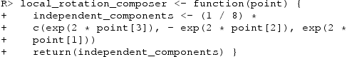
where the parameter 1/8 is chosen to create a small rotation for illustrative purposes. Next, the error model can be specified with a function which defines $\mathrm{\Phi }(\mathit{\epsilon })$ (given by Equation (2(2) $\mathrm{\Phi }(\mathit{a})=\left(\begin{array}{ccc}0& -a_3& a_2\\ a_3& 0& -a_1\\ -a_2& a_1& 0\end{array}\right);$(2) )) which acts on the vector of errors for an explanatory point $\mathit{x}$:

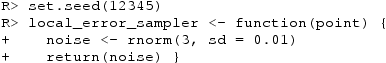
in which a very small standard deviation is used so that the rotation model dominates, and in this example the error distribution is independent of the point $\mathit{x}$. Finally, $\mathit{Y}$ is obtained using the simulate_regression() function, which returns the response points corresponding to the specified explanatory_points, given a model for local rotations (local_rotation_composer) and an error term distribution (local_error_sampler).

Note that data may be simulated with errors which have a von Mises–Fisher distribution using the function simulate_regression() as above, but with the local_error_sampler() specified to return a vector of zeroes (no errors). Then errors may be added by using the function rmovMF() in the movMF library.

We generally obtain predictions at a new matrix of points, which can be specified by the user, but for simplicity here we will use the existing $\mathit{X}$.

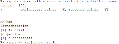
The concentration argument needs to be specified. It is a non negative scalar whose reciprocal is proportional to the square of the Euclidean bandwidth, that can be arbitrarily chosen by the user, or else chosen by cross-validation, using the function cross_validate_concentration(). This function uses optimize() to search for κ in a positive interval, with the upper bound set by concentration_upper_bound (set to 10 by default) to minimize Equation (5(5) $\sum _{i=1}^n||{\hat{\mathit{y}}}_i^{(i)}-{\mathit{y}}_i|{|}^2$(5) ). Given the matrices of explanatory and response points, cross_validate_concentration() returns the optimal choice of κ (concentration) and the corresponding objective value (objective). In our illustrative example we have:

If no scheme for weighting observed data is specified, cross_validate_concentration() uses as the weights_generator the function weight_explanatory_points() that, given the matrices of m evaluation_points, n explanatory_points and a concentration parameter, returns an $n\times m$ weight matrix ${\mathit{W}}_{\kappa }$ (whose jth column contains the weights assigned to the explanatory points whilst considering the jth evaluation point). Within the package the default kernel is $K_{\kappa }({\mathit{x}}_i^T\mathit{x})=\exp (\kappa ({\mathit{x}}_i^T\mathit{x}-1))$, which is a rotationally symmetric function with maximum at $\mathit{x}$. It can be assigned by using the aforementioned built-in function as follows:

Then, using the fit_regression() function, we can obtain the predicted values $\hat{\mathit{Y}}$, corresponding to the evaluation_points:

Other than the main arguments discussed above (evaluation_points, explanatory_points, response_points and concentration), when using the function fit_regression() it is possible to specify some additional, optional arguments that are briefly described in Table 2. Note that the function cross_validate_concentration() also has all the arguments and options listed in Table 2, therefore the best choice of κ will also depend on: the specific kernel used; the number of iterations; whether a first- or second-order expansion is used; and whether reflections are allowed. We also note that the function fit_regression() allows the user to exploit the doParallel package as this was seen to speed the computations by about 20%, but this option has not been implemented for cross_validate_concentration() since no such improvement was observed.

Table 2. Optional arguments – and their defaults – of the fit_regression() function.

argument	default	options and meaning
weights_generator	weight_explanatory_points	function to return diagonal entries of the matrix $\mathit{W}$ given matrix arguments evaluation_points and explanatory_points, and a concentration (κ)
number_of_expansion_terms	1	options are 1, which uses (4(4) ${\hat{\mathit{R}}}_{\mathit{x}}=\underset{{\mathit{R}}_{\mathit{x}}\in \mathrm{SO}(d)}{\mathrm{argmin}}\sum _{i=1}^n||{\mathit{y}}_i-{\mathit{R}}_{\mathit{x}}^T{\mathit{x}}_i|{|}^2{K}_{\kappa }\left({\mathit{x}}_i^T\mathit{x}\right),$(4) ), or 2, which uses (6(6) $\underset{{\mathit{R}}_{\mathit{x}}\in \mathrm{SO}(d),{\mathsf{\text{D}}}_{{\mathit{S}}_{\mathit{x}}}^{(1)}({\mathit{x}}_i,\mathit{x})\in {\mathrm{Skew}}_d}{\mathrm{argmin}}\sum _{i=1}^n{\left||{\mathit{y}}_i-{\mathit{R}}_{\mathit{x}}^T{\{{\mathit{I}}_d+{\mathsf{\text{D}}}_{{\mathit{S}}_{\mathit{x}}}^{(1)}({\mathit{x}}_i,\mathit{x})\}}^T{\mathit{x}}_i|\right|}^2{K}_{\kappa }\left({\mathit{x}}_i^T\mathit{x}\right)$(6) )
number_of_iterations	1	This is M, the number of iterations, as described in Section 3.2
allow_reflections	FALSE	TRUE replaces the matrix $\mathbf{\Delta }$ by the identity $\mathit{I}$, so that $\mathit{R}=\mathit{V}{\mathit{U}}^T$ – possibly an ‘improper’ rotation – may include reflections. The default prohibits $|\mathit{R}|=-1$ which would indicate that the solution contains a reflection.

Consequently, the output of the function fit_regression() is a list of length equal to the number_of_iterations M, in which, for $m=1,\dots ,M$, the mth component includes two objects, the $m\times d$ matrix of fitted values of $\mathit{Y}$ corresponding to the evaluation_points (fitted_response_points), and the data matrix ${\hat{\mathit{X}}}_m$ (explanatory_points). In our example, we use the default value of the number_of_iterations (which is set to 1), therefore to get the fitted response matrix $\hat{\mathit{Y}}$ we write:

The mean of the residual sum of squares is somewhat smaller than the leave-one-out estimate:

Two other useful functions that have been included in the package are:

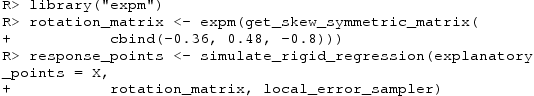
• get_skew_symmetric_matrix(), whose argument is a vector (say $\mathit{a}$) of length 3 and returns a matrix given by $\mathbf{\Phi }(\mathit{a})$ as in Equation (2(2) $\mathrm{\Phi }(\mathit{a})=\left(\begin{array}{ccc}0& -a_3& a_2\\ a_3& 0& -a_1\\ -a_2& a_1& 0\end{array}\right);$(2) );

• simulate_rigid_regression(), which is similar to simulate_regression(), but with the argument local_rotation_composer replaced by a rotation_matrix $\mathit{R}$. The error structure is the same, so this generates $\mathit{y}$ values according to model (1(1) ${\mathit{y}}_i=\exp (\mathrm{\Phi }({\mathit{\epsilon }}_i)){\mathit{R}}^T{\mathit{x}}_i\mathbf{,}i=1,\dots ,n,$(1) ).

For example, after loading the library expm [36], using these two functions and keeping the same explanatory points and error term as before, we can built a rotation matrix and generate the response points as follows:

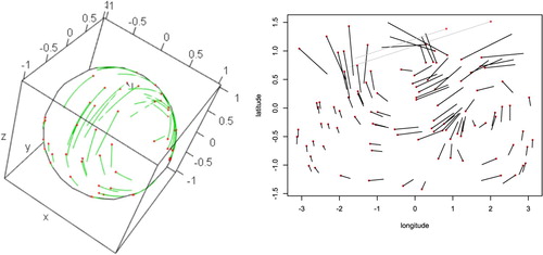
With these parameter settings (local_error_sampler error SD set to 0.01), it is easy to visualize the rotation models in a graphical plot. We can either use a projection of the sphere onto the plane, or a 3-D plot using the package rgl [37] as follows:

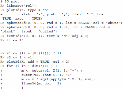
The projection plot can be obtained by first converting to spherical coordinates:

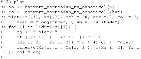
We have drawn grey lines to indicate that the shortest path is ‘around the back’. For our simulation, the above two plots are shown in Figure 1.

Figure 1. $\mathit{X}$ (red points) and fitted $\hat{\mathit{Y}}$ pairs using rgl (left) and a latitude–longitude projection in radians (right).

5.2.1. World magnetic field model

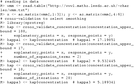
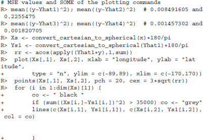
There are hundreds of observatories around the world which record the geomagnetic field every hour. The locations of these observatories can be represented as points on the sphere, as can the 3-d vector of the magnetic field observations, after suitable normalization. We use these as our explanatory points and response values, respectively. The World Magnetic Model (WMM), which was developed jointly by NCEI (formerly NGDC) and the British Geological Survey, is based on very high-order spherical polynomials fitted to such data, and can be used to predict the magnetic field at any place on the planet. Since the Earth has a molten iron core the magnetic field varies over time, and the WMM is updated every few years. To illustrate the flexibility of our nonparametric rotation model, we use historical data from 90 observatories, with recordings taken at 1am on 1st January 2008. The data are available in IAGA format from www.ngdc.noaa.gov/geomag/data.shtml, and the data we use is plotted in Figure 2.

Figure 2. Latitude–longitude projection (in degrees) for geomagnetic observations taken at 1am on 01/01/2008. Top left: locations of observatories (points) connected to response values by lines. Top right: equally spaced design points connected to predicted values for fitted first-order model. In the bottom two rows, the observatory locations are shown as points with size in relation to residuals (see R code). Middle left: rigid rotation model connecting locations to predicted values; Middle right: locations connected to predicted values using first-order model. Bottom left: iterated (first-order) solution, with 20 iterations. Bottom right: second-order solution. Connecting lines are shown in grey when the shortest distance is ‘around the back’.

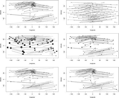
We first choose the smoothing parameter by leave-one-out cross-validation. The resulting value of κ is found to be 17.19. We also investigate the second-order model (6(6) $\underset{{\mathit{R}}_{\mathit{x}}\in \mathrm{SO}(d),{\mathsf{\text{D}}}_{{\mathit{S}}_{\mathit{x}}}^{(1)}({\mathit{x}}_i,\mathit{x})\in {\mathrm{Skew}}_d}{\mathrm{argmin}}\sum _{i=1}^n{\left||{\mathit{y}}_i-{\mathit{R}}_{\mathit{x}}^T{\{{\mathit{I}}_d+{\mathsf{\text{D}}}_{{\mathit{S}}_{\mathit{x}}}^{(1)}({\mathit{x}}_i,\mathit{x})\}}^T{\mathit{x}}_i|\right|}^2{K}_{\kappa }\left({\mathit{x}}_i^T\mathit{x}\right)$(6) ) and the iterated solution (9(9) ${\hat{\mathit{R}}}_{M,\mathit{x}}^T\dots {\hat{\mathit{R}}}_{1,\mathit{x}}^T\mathit{x}.$(9) ), again choosing the smoothing parameters by cross-validation. It should be noted that the second-order model is computationally intensive and takes many times longer to compute than even 20 iterations of the first-order iterated solution. For example, with 100 observations, the second-order model took about 200 times longer than 20 iterations of the first-order iterated solution. As with many cross-validation functions, there is the possibility of local minima. This can be mitigated by trying a few different upper bounds. After finding a good choice of κ for the first-order model this value can provide an upper bound for both iterated solutions and second-order models, since their optimal smoothing parameters will, in general, be less.

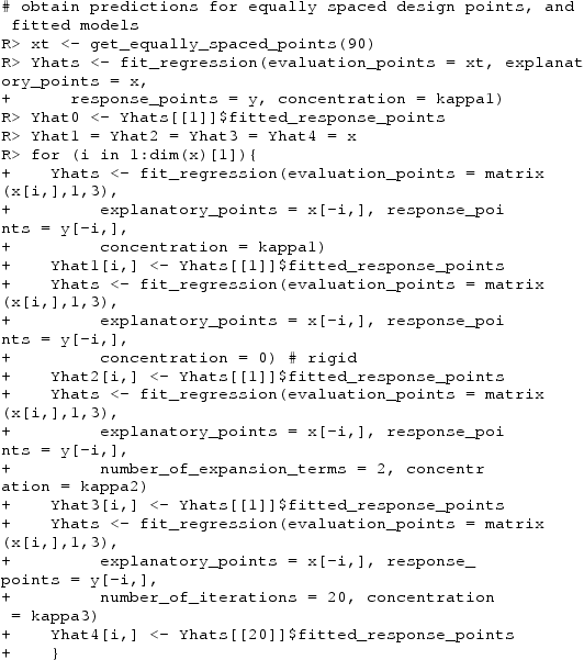
Using these values of κ we can fit each model to ‘new’ design points which are equally spaced on the sphere, and to the data, obtaining predictions by leave-one-out, and – for comparison – to a rigid rotation model ($\kappa =0$).

The fitted y values can be compared to the responses, with mean squared errors of 0.0085 and 0.226 for the flexible and rigid rotation models, respectively. For comparison, the second-order model has mean-squared error 0.0015, and the iterated solution 0.0018. Choosing the number of iterations could be done by cross-validation, but provided κ is suitably chosen, the best fit will often be for very large values of M. So, in practice we recommend trying a few values (perhaps in increments of 5), and selecting the smallest which leads to a useful improvement over the non-iterated solution (M = 1). We note that allowing reflections in the standard (first-order, M = 1) case gives a cross-validated mean squared error of 0.0072 with $\kappa =22.3$, which is quite similar to the performance when reflections are prohibited so we have not pursued this option further in these illustrations.

We can visualize the fitted models using a latitude–longitude projection. It is clear that the rigid model lacks the flexibility required for the data. For the first-order solution, the selected value of κ leads to a reasonable fit for those observations which are more dense, but – as can be seen in Figure 2 – with larger residuals for those near the equator where the observatories are more sparse. Both the second-order model and the iterated solution make improvements on this, albeit at the expense of more computational effort.

6. Summary and discussion

Regression when data are located on a sphere is a classical statistical problem attracting interest from many applied fields, in particular in Earth Sciences. As a specific case, many disciplines need to consider circular–circular data, that are of interest when studying directions, for example, in metereology and animal behaviour studies. It has been observed that parametric approaches often result in solutions which are too rigid and do not fully describe or interpret the data. As a consequence, non-parametric approaches are gaining in popularity, giving rise to the need for a package of interest to nonparametric practitioners belonging to various scientific disciplines. In this paper, the nprotreg package for the implementation of non-parametric spherical–spherical regression methods proposed by [12] is described. The method is based on local estimation of rotation matrices, assuming that a single rotation is unable to explain the regression for the whole dataset, and rotation matrices exist that explain data dependence in a local manner. The content of the package is divided into two parts: the conversion functions, that preliminarily make accessible other data formats, and the proper regression ones. Finally, the package provides useful tools for simulating sphere–sphere data according to non-rigid rotation models, including a rigid rotation as a specific case.

The results in this paper were obtained using  4.0.3. itself and all packages used are available from the Comprehensive Archive Network (CRAN) at https://CRAN.R-project.org/.

Disclosure statement

No potential conflict of interest was reported by the author(s).

Notes

1 We will not specify the origin package for functions belonging to base, stats and nprotreg.

References

- Hamsici O, Martinez AM. Spherical-homoscedastic distributions: the equivalency of spherical and normal distributions in classification. J Mach Learn Res. 2007;8:1583–1623.
- Dryden IL, Mardia KV. Statistical shape analysis: with applications in R. 2nd ed. New York: John Wiley & Sons; 2016.
- Chang T, Ko D, Royer JY, et al. Regression techniques in plate tectonics. Stat Sci. 2000;15:342–356.
- Mackenzie JK. The estimation of an orientation relationship. Acta Crystallogr. 1957;10:61–62.
- Wahba G. Problem 65-1: A least squares estimate of spacecraft attitude. SIAM Rev. 1965;7:409.
- Shin G, Chun J. Vision-based multimodal human computer interface based on parallel tracking of eye and hand motion. 2007 International Conference on Convergence Information Technology (ICCIT 2007); IEEE; 2007. p. 2443–2448.
- Witze A. Earth's magnetic field is acting up and geologists don't know why. Nature. 2019;565(7738):143–144.
- Chang T. Spherical regression. Ann Stat. 1986;14:907–924.
- Rivest L. Spherical regression for concentrated Fisher–von Mises distributions. Ann Stat. 1989;17:307–317.
- Downs T. Spherical regression. Biometrika. 2003;90:655–668.
- Di Marzio M, Panzera A, Taylor CC. Nonparametric regression for spherical data. J Am Stat Assoc. 2014;109:748–763.
- Di Marzio M, Panzera A, Taylor CC. Nonparametric rotations for sphere-sphere regression. J Am Stat Assoc. 2019;114:466–476.
- Core Team:. A language and environment for statistical computing. Vienna, Austria: Foundation for Statistical Computing; 2019. https://www.R-project.org/.
- Agostinelli C, Lund U. CircStats: Circular statistics, from topics in circular statistics. 2018. https://CRAN.R-project.org/package=CircStats.
- Agostinelli C, Lund U. circular: Circular statistics. 2017. https://r-forge.r-project.org/projects/circular/.
- Oliveira M, Crujeiras RM, Rodríguez-Casal A. NPCirc: an R package for nonparametric circular methods. J Stat Softw. 2014;61(9):1–26.
- Fitak RR, Johnsen S. Bringing the analysis of animal orientation data full circle: model-based approaches with maximum likelihood. J Exp Biol. 2017;220(3):3878–3882.
- Fernandez-Duran JJ, Gregorio-Dominguez MM. CircNNTSR: an R package for the statistical analysis of circular, multivariate circular, and spherical data using nonnegative trigonometric sums. J Stat Softw. 2016;70(6):1–19.
- Barragan S, Fernandez MA, Rueda C, et al. isocir: an R package for constrained inference using isotonic regression for circular data, with an application to cell biology. J Stat Softw. 2013;54(4):1–17.
- Nadarajah S, Zhang Y. Wrapped: an R package for circular data. PLoS ONE. 2017;12(12):1–26.
- Ghazanfarihesari A, Sarmad M. CircOutlier: Detection of outliers in circular-circular regression. 2016. https://CRAN.R-project.org/package=CircOutlier.
- Tsagris M, Athineou G, Sajib A, et al. Directional: Directional statistics. 2019. https://CRAN.R-project.org/package=Directional.
- Hornik K, Grün B. movMF: an R package for fitting mixtures of von mises-fisher distributions. J Stat Softw. 2014;58(10):1–31.
- Robotham A. sphereplot: Spherical plotting. 2013. https://CRAN.R-project.org/package=sphereplot.
- Hijmans RJ, Williams E, Vennes C. geosphere: Spherical trigonometry; 2017. https://CRAN.R-project.org/package=geosphere.
- Hornik K, Feinerer I, Kober M, et al. Spherical k-means clustering. J Stat Softw. 2012;50(10):1–22.
- Stanfill B, Hofmann H, Genschel U. rotations: an R package for SO(3) data. R J. 2014;6:68–78.
- Oh HS, Kim D. SpherWave: Spherical wavelets and sw-based spatially adaptive methods. 2007. http://stat.snu.ac.kr/heeseok/SpherWave.html.
- Nolan JP. SphericalCubature: numerical integration over spheres and balls in n-dimensions; multivariate polar coordinates. 2017. https://CRAN.R-project.org/package=SphericalCubature.
- Robeson S, Li A, Huang C. SphericalK: Spherical k-function. 2015. https://CRAN.R-project.org/package=SphericalK.
- Pewsey A. Directional statistics for wildfires. In Ley C, Verdebout T, editors. Applied directional statistics with R: An overview. Boca Raton, Florida: Chapman and Hall/CRC Press; 2018.
- Mardia KV, Jupp PE. Directional statistics. Chichester, UK: John Wiley; 2000.
- Di Marzio M, Taylor CC. On boosting kernel regression. J Stat Plan Inference. 2008;138:2483–2498.
- Euler L. Nova methodus motum corporum rigidorum determinandi. Novi Commentari Acad Imp Petrop. 1775;20:208–238.
- Cheng H, Gupta KC. A historical note on finite rotations. J Appl Mech. 1989;56:139–145.
- Goulet V, Dutang C, Maechler M, et al. expm: Computation of the matrix exponential, logarithm, sqrt, and related quantities. 2018. https://CRAN.R-project.org/package=expm.
- Adler D, Murdoch D. rgl: 3d visualization using opengl. 2018. https://r-forge.r-project.org/projects/rgl/.