Comparison of parametric and semiparametric survival regression models with kernel estimation

Abstract

The modelling of censored survival data is based on different estimations of the conditional hazard function. When survival time follows a known distribution, parametric models are useful. This strong assumption is replaced by a weaker in the case of semiparametric models. For instance, the frequently used model suggested by Cox is based on the proportionality of hazards. These models use non-parametric methods to estimate some baseline hazard and parametric methods to estimate the influence of a covariate. An alternative approach is to use smoothing that is more flexible. In this paper, two types of kernel smoothing and some bandwidth selection techniques are introduced. Application to real data shows different interpretations for each approach. The extensive simulation study is aimed at comparing different approaches and assessing their benefits. Kernel estimation is demonstrated to be very helpful for verifying assumptions of parametric or semiparametric models and is able to capture changes in the hazard function in both time and covariate directions.

Keywords:

• Survival analysis
• hazard function
• Kernel estimation
• simulations
• Cox model

1. Introduction

Survival analysis belongs to a set of statistical methods that deals with the description of time from an initial event until the occurrence of an observed event, i.e. time-to-event data. Most of the applications can be found in medical research. However, it is often also used in other fields, such as economics or engineering. Usually, the event of interest is only partially observed due to the earlier occurrence of a censored event. In such studies, the estimation of the survival and hazard function has received considerable attention. Estimation of the survival function is essential, both as a preliminary analysis and as the basic building block for further analyses such as regression models. The estimator of the survival function suggested by Kaplan and Meier [1] was an important milestone in survival analysis. However, further developments have shown that the hazard function is just as important as the survival function because it provides basic concepts for the statistical modelling of censored data. The hazard function is defined as the instantaneous probability of a given event occurring at the next time instant: $\lambda (t)=\underset{\mathrm{\Delta }t\to \mathrm{\infty }}{lim}\frac{P(t\le T<t+\mathrm{\Delta }t|T\ge t)}{\mathrm{\Delta }t}.$The survival and hazard functions provide an alternative but equivalent characterizations of the survival time distribution. Given the survival function, the density can always be obtained, and the hazard function calculated as it is shown below. The survival function can always be determined from the given hazard function. Both functions should be considered together for more beneficial interpretation. The hazard function captures the decreasing speed of the survival curve and is a measure of instantaneous potential, whereas the survival curve is a cumulative measure over time.

Several methods have been proposed in the literature to estimate this function. Estimation by non-parametric methods has the advantage of flexibility because no formal assumptions are needed about the mechanism that generates the sample order or the randomness. The most effective techniques are smoothed estimators due to the properties of the hazard function. Kernel estimation is one of many possibilities. Its advantage is that no assumptions about the distribution of survival times are necessary. Kernel smoothing is based on a real function $K(\cdot )$ called a kernel and a smoothing parameter h called the bandwidth. See, for example, books [2] or [3] for details.

In practice, survival time will often be affected by some covariates such as age, sex, or tumour marker. The influence of these covariates is usually explained using regression models. These models are based on a different estimation of the conditional hazard function defined as $\lambda (t|x)=\underset{\mathrm{\Delta }t\to \mathrm{\infty }}{lim}\frac{P(t\le T<t+\mathrm{\Delta }t|T\ge t,\mathbf{X}=\mathbf{x})}{\mathrm{\Delta }t}.$Parametric models [see][4] are useful in the case of a known survival time distribution. However, this distribution is often unknown, and its dependence on time is estimated by non-parametric methods. In the case of semiparametric models, the influence of covariates is estimated parametrically. A frequently used method has been the model suggested by Cox [5]. This model is based on the assumption of the proportionality of hazards, which is the hazard ratio between two sets of covariates is constant over time. Also, the exponential dependence of the hazard on covariates is assumed. In many cases, these assumptions are too restrictive. Other semiparametric models, such as Aalen's additive model [see][6] are also restrictive in many situations. The alternative approach is to use either spline or kernel smoothing. Comprehensive approaches to estimate the hazard function using splines are given in [7] and [8].

Kernel smoothing in the case of the hazard function can be tackled using two different approaches. Consequently, two types of estimators can be considered. The first type of estimator is referred to as an external type. This estimator is obtained as the ratio of estimators of density to a survival function. The external estimator for uncensored data and the unconditional case was introduced by Watson and Leadbetter [9,10]. Other authors made the extension to censored data, e.g. [11]. Nielsen and Linton [12] proposed the external estimator for the conditional hazard function using a counting process. Spierdijk [13] and Kim et al. [14] studied the local linear estimator for a conditional case.

The second type of estimator is referred to as an internal type and is based on the smoothing of an estimator for the cumulative hazard function. Watson and Leadbetter [9,10] introduced this estimator of the unconditional hazard function for uncensored data. The extension to censored data was studied by various authors, e.g. [15] or [16]. The internal estimator for the conditional hazard function using a counting process was described by Li [17]. Van Keilegom and Veraverbeke [18] used Gasser-Müller weights to obtain the internal estimator of the conditional hazard function in a fixed design model.

Extending kernel estimators by assuming dependence between covariates was proposed by Linton et al [19] with restriction to additive or multiplicative hazard functions. These results were extended by Wolter [20], who introduced a simulation study examining the effect of dependence on finite sample properties of the relevant estimators.

The analysis of censored data remains a cornerstone of biostatistical practice, and therefore, the literature on this broad topic is incredibly rich. On the other hand, the articles related to applications are often restricted to the best-known survival models that are also available in the standard statistical software. The paper aims to show the weaknesses of these models compared with the kernel estimation. The kernel smoothing is based on a natural idea but provides a remarkable view on data especially in the presence of a covariate. It can serve as a tool for determining the appropriate model, subsequent data manipulation, or final interpretation.

The paper is organized as follows. Both external and internal kernel estimators of the conditional hazard function based on Nadaraya–Watson type weights for a random design model are proposed. Methods for choosing the smoothing parameters are then introduced. In Section 3, the best-known parametric and semiparametric models are summarized. Standard models without further extensions are focused on. These models, along with kernel estimators, are applied to breast cancer data in Section 4. Section 5 is devoted to a simulation study where data for a specified conditional hazard function are simulated. The aim of the simulation study is to compare kernel estimates and (semi)parametric models in different situations. Finally, some conclusions are drawn in Section 6.

All analyses were performed using R software version 3.4.3 [21] and MATLAB version 2015b.

2. Kernel estimation

Let T denote a nonnegative random variable representing the survival time of an individual with the survival function $\overline{F}(\cdot )$ and the density $f(\cdot )$. Let C be a right censoring variable independent of T with the survival function $\overline{G}(\cdot )$ and the density $g(\cdot )$. Define the observable random variable $Y=min(T,C)$ and the censoring indicator $\delta =I(T\le C)$ where $I(\cdot )$ denotes the indicator function. Let $\overline{L}(\cdot )$ and $l(\cdot )$ denote the survival function and the density of Y, respectively. From the independence of T and C it follows that $\overline{L}(t)=P(Y\ge t)=P(T\ge t\wedge C\ge t)=\overline{F}(t)\overline{G}(t).$Additionally, $l(\cdot ,\cdot )$ denotes the density of $(Y,\delta )$ and $r(\cdot )=l(\cdot ,1)$ is the subdensity of the uncensored observation that can be expressed in the form $r(t)=f(t)\overline{G}(t).$The unconditional hazard function $\lambda (t)$ can be written as the ratio of the density to the survival function of survival time T, and then rewritten as the ratio of the subdensity of the uncensored observation to the survival function of the observable time Y, i.e. (1) $\lambda (t)=\frac{f(t)}{\overline{F}(t)}=\frac{f(t)\overline{G}(t)}{\overline{L}(t)}=\frac{r(t)}{\overline{L}(t)}.$(1) Let X additionally denote a covariate with the density $s(x)$. For simplicity, assume that X is a scalar, although extension to a case of higher dimension is possible. Also, assume a fixed covariate, i.e. constant over time. Let $\overline{F}(\cdot |x)$, $\overline{G}(\cdot |x)$, and $\overline{L}(\cdot |x)$ denote the conditional survival functions of T, C, and Y, respectively, given X = x. Functions $\overline{f}(\cdot |x)$, $\overline{g}(\cdot |x)$, and $\overline{l}(\cdot |x)$ are corresponding densities. The subdensity of the uncensored observation given X = x is $r(t|x)=f(t|x)\overline{G}(t|x)$.

The conditional hazard function given X = x can be written similarly to the unconditional case as (2) $\lambda (t|x)=\frac{f(t|x)}{\overline{F}(t|x)}=\frac{f(t|x)\overline{G}(t|x)}{\overline{L}(t|x)}=\frac{r(t|x)}{\overline{L}(t|x)}.$(2) The observed data are $(Y_i,{\delta }_i)$ in the unconditional case or $(X_i,Y_i,{\delta }_i)$ in the conditional case, $i=1,\dots ,n$, with the same distribution as $(Y,\delta )$ and $(X,Y,\delta )$, respectively.

The basic idea of kernel estimations can be expressed as follows: the value of the unknown function at some point can be estimated as a local weighted average of known observations in the neighbourhood of this point. The kernel function $K(\cdot )$ plays the role of the weight, and the bandwidth h determines the size of the neighbourhood. The kernel is usually a function with properties of the probability density, i.e. $K(\cdot )$ is a nonnegative function on $\mathbb{R}$ which is symmetric and integrated to one. Several types of kernel functions are commonly used, such as Epanechnikov kernel $K(u)=\frac{3}{4}(1-u^2)$ with a bounded support on the interval $[-1,1]$ or Gaussian kernel $K(u)=\frac{1}{\sqrt{2\pi }}{\mathrm{e}}^{-\frac{u^2}{2}}$ with an unbounded support.

In the case of estimation of conditional function (density, distribution or hazard), the observations in the neighbourhood of the point are considered separately in the direction of the covariate and survival time. In general, two different kernel functions with different bandwidths can be considered. Whereas the quality of kernel estimates with a fixed kernel depends mainly on the choice of the bandwidths, only the case of the same kernel function in both directions will be described. Next, denote $h_x$ and $h_t$ bandwidths in the direction of the covariate and survival time, respectively. These bandwidths are dependent on n. Assume that the non-random sequences of positive numbers $\{h_x=h_x(n)\}$ and $\{h_t=h_t(n)\}$ satisfies $\underset{n\to \mathrm{\infty }}{lim}{h}_x(n),\underset{n\to \mathrm{\infty }}{lim}{h}_t(n)=0,\underset{n\to \mathrm{\infty }}{lim}n{h}_x(n)h_t(n)=\mathrm{\infty }$. Finally, denote $W(\cdot )$ a kernel distribution function, i.e. $W(t)={\int }_{-\mathrm{\infty }}^{t}K(u)\mathrm{d}u$.

2.1. External estimator

One way to estimate the conditional hazard function $\lambda (t|x)$ is to replace the numerator and denominator in (2(2) $\lambda (t|x)=\frac{f(t|x)}{\overline{F}(t|x)}=\frac{f(t|x)\overline{G}(t|x)}{\overline{L}(t|x)}=\frac{r(t|x)}{\overline{L}(t|x)}.$(2) ) with their kernel estimators $\hat{r}(t|x)$ and $\hat{\overline{L}}(t|x)$. The kernel estimation of the conditional function combines the kernel estimation of the unconditional function and the kernel regression. An approach based on Nadaraya–Watson smoothing [see][2] is used.

The Nadaraya–Watson weights are defined by $w_i(x)=\frac{K\left(\frac{x-X_i}{h_x}\right)}{{\displaystyle \sum _{j=1}^{n}K\left(\frac{x-X_j}{h_x}\right)}},i=1,\dots ,n.$The kernel estimator of conditional subdensity of the uncensored observation $r(t|x)$ is given by $\hat{r}(t|x)=\frac{1}{h_t}{\displaystyle \sum _{i=1}^n{w}_i(x)K\left(\frac{t-Y_i}{h_t}\right){\delta }_i}$and the kernel estimator of conditional survival function of the observable time is (3) $\hat{\overline{L}}(t|x)=\sum _{i=1}^n{w}_i(x)W\left(\frac{Y_i-t}{h_t}\right).$(3) The external kernel estimator of conditional hazard function is defined as ${\hat{\lambda }}_E(t|x)=\frac{\hat{r}(t|x)}{\hat{\overline{L}}(t|x)}=\frac{\frac{1}{h_t}{\displaystyle \sum _{i=1}^n{w}_i(x)K\left(\frac{t-Y_i}{h_t}\right){\delta }_i}}{{\displaystyle \sum _{i=1}^n{w}_i(x)W\left(\frac{Y_i-t}{h_t}\right)}}.$

2.2. Internal estimator

The alternative approach to estimate the conditional hazard function is based on a convolution of the kernel function with a non-parametric estimator of the conditional cumulative hazard function.

Assume now that $Y_{(1)},Y_{(2)},\dots ,Y_{(n)}$ are ordered $Y_1,Y_2,\dots ,Y_n$, i.e. $Y_{(1)}\le Y_{(2)}\le \dots \le Y_{(n)}$, ${\delta }_{(1)},{\delta }_{(2)},\dots ,{\delta }_{(n)}$ are corresponding censoring indicators and $X_{(1)},X_{(2)},\dots ,X_{(n)}$ are corresponding covariates.

The non-parametric estimator of the conditional cumulative hazard function was introduced by Beran [22], who first studied the estimation of the cumulative hazard function in the presence of a covariate with randomly censored survival data. The main idea is the use of smoothing over the covariate space. The estimator of conditional cumulative hazard function is used in the form $\hat{\mathrm{\Lambda }}(t|x)=\{\begin{array}{ll}0& t\le Y_{(1)},\\ {\displaystyle \sum _{i:Y_{(i)<t}}\frac{{\delta }_{(i)}{w}_{(i)}(x)}{1-{\displaystyle \sum _{j=1}^{i-1}{w}_{(j)}(x)}}}& t>Y_{(1)}\end{array}$where $w_{(i)}(x)$ are Nadaraya–Watson weights corresponding to $Y_{(i)}$. Notice, that if all weights are equal to $\frac{1}{n}$, this estimator will be reduced to the Nelson–Aalen estimator [see][23].

The internal conditional estimator of the conditional hazard function is defined consequently as ${\hat{\lambda }}_I(t|x)=\frac{1}{h_t}{\displaystyle \sum _{i=1}^{n}K\left(\frac{t-Y_{(i)}}{h_t}\right)\frac{{\delta }_{(i)}{w}_{(i)}(x)}{1-{\displaystyle \sum _{j=1}^{i-1}{w}_{(j)}(x)}}.}$

2.3. Selection of bandwidths

The fundamental problem in kernel smoothing theory is the choice of suitable bandwidths. If the kernel function is chosen, the quality of the estimate will be dependent primarily on bandwidths. Notice that two bandwidths are needed in the conditional case. These smoothing parameters have a different role in the quality of the estimate. The parameter $h_x$ influences the smoothing of the estimate in the direction of the covariate. The parameter $h_t$ influences instead of that the quality of the estimate in the direction of time. However, the choice of parameters is not independent. Therefore, selecting bandwidths for the conditional case is even more difficult than for unconditional functions.

If the data distribution is known, the optimal smoothing parameters could be determined [see][13,17,24]. In practice; however, data distribution is unknown. Therefore, bandwidths must be estimated. To select bandwidths, two methods are applied. The notion behind these methods is similar for both types of estimators. A joint label for the internal and external estimator of the conditional hazard function is used, namely $\hat{\lambda }(t|x)$. Where necessary, the potential differences between estimators will be indicated.

The computational complexity of methods for selecting bandwidths is high in the conditional case. Computational time demands dramatically increase with the size of the data set. This handicap could be a motive for simplifying assumptions. One such an assumption is the equality of both parameters, i.e. $h_x=h_t$. However, this may not be suitable due to the different roles each parameter has.

Another option is offered for the external estimator. It is possible to consider estimates separately in the numerator and the denominator and choose their parameters [see][25]. In this case, there would be four generally different smoothing parameters. This approach does not have to provide good results. Although the smoothing parameters are suitable for estimating the conditional survival function and the estimate of the conditional subdensity, they may not be suitable choices for the ratio of these estimates. Conversely, this method is helpful for software with implemented functions for the kernel estimation of the density and the distribution function.

In Appendix, no limiting assumptions are considered, and two methods of bandwidths selection are introduced, namely the cross-validation method and the maximum-likelihood method. Both mentioned estimators included both bandwidth selection methods are now implemented in the R package kernhaz.

3. Overview of other approaches

The aim of this section is to briefly summarize some other approaches for estimating conditional hazard. These models are described in many books and articles [see, e.g.][4,23], are also available in standard statistical software and especially often used in practice. Each of these models has some assumptions which are often overlooked. It is necessary to note models considered in this section are only a fraction of existing survival models.

3.1. Parametric models

A parametric survival model is one in which survival time is assumed to follow a known distribution. Accelerated failure time (AFT) models [see][4,26] shall be considered. The underlying assumption for AFT models is that the effect of covariates is proportional to survival time. Specifically, it can be written as $\log T=\psi (X)+\epsilon ,$where ψ is an unknown function and ε is a random error. Most AFT models assume a linear function of a covariate. Often considered distributions are exponential, Weibull, or lognormal. AFT models are common in industrial applications where multiplicative time scales often make sense. R function survreg in the package survival can fit a range of models with various distributions. AFT models based on a non-parametric error term were proposed in [27]. The effect of the covariate in the AFT model is interpreted using a time ratio (TR) expressing the proportion of the survival time change from a one-unit increase in the covariate. TR greater than one for the covariate implies that this covariate prolongs the time to an event, while TR less than one indicates that an earlier event is more likely.

One other general family of parametric survival models is parametric proportional hazard (PH) models. These models are similar to the Cox model discussed below, except that baseline hazard is estimated parametrically. The effect of the covariate in the PH model is interpreted using a hazard ratio (HR) expressing the proportion of the hazard change from a one-unit increase in the covariate. HR greater than one means that the event is more likely to occur, and HR less than one means that an event is less likely to occur.

3.1.1. Weibull model

The conditional hazard function for the Weibull model can be written in the form $\lambda (t|x)=\nu \mu t^{\mu -1}{\mathrm{e}}^{\beta x},$where ν is a scale parameter, μ a shape parameter, and β a regression coefficient. A special case for $\mu =1$ is the exponential model. Interpretation of this model is possible using both AFT and PH models. TR can be obtained as $\mathrm{TR}=\exp (-\frac{\beta }{\mu })$ and HR as $\mathrm{HR}=\exp (\beta )$.

3.1.2. Lognormal model

The conditional hazard function in this case is given by $\lambda (t|x)=\frac{\frac{1}{\sigma t}\varphi \left(\frac{\log t-\beta x-\mu }{\sigma }\right)}{\mathrm{\Phi }\left(\frac{\beta x+\mu -\log t}{\sigma }\right)},$where μ is a location parameter, σ a scale parameter, and β a regression coefficient. Time ratio is given by $\mathrm{TR}=\exp (\beta )$.

3.2. Semiparametric models

The semiparametric models are without any survival time distribution assumption, but other assumptions remain (e.g. the relationship between survival time and the covariate or the proportionality of hazards).

3.2.1. Cox proportional hazard model

The most frequently used model in practice is based on the proportionality of hazards, i.e. the hazard ratio is constant over time. This model was introduced by Cox [5]. Furthermore, the conditional hazard function is given by $\lambda (t|x)={\lambda }_0(t){\mathrm{e}}^{\beta x},$where ${\lambda }_0(t)$ is the baseline hazard function and β is the regression coefficient. The baseline hazard is estimated by the non-parametric method, while the estimation of the parameter β is based on maximizing the partial likelihood function. The conditional hazard function is not well graphically presentable for these estimators, but smoothing techniques can be used. The hazard ratio is given by $\mathrm{HR}=\exp (\beta )$. Note that exponential dependence on the covariate is assumed for the conditional hazard function. The Cox model is available with most statistical software. In R, this model is fitted by the function coxph in the package survival.

The popularity of the Cox model may lie in the fact that to identify the effect of a covariate on the risk of death it is not necessary to specify an estimation of the baseline hazard rate. This popularity has lead to the development of many modifications (generalizations or extensions), see [28,29] or [30].

3.2.2. Gray's model

Flexible extension of the Cox proportional hazard model was introduced by Gray [31]. The conditional hazard function for this model is in the form $\lambda (t|x)={\lambda }_0(t){\mathrm{e}}^{\beta (t)x}.$Thus, contrary to Cox model, the regression coefficient β is time-varying. Gray's model uses penalized B-splines to model this effect. This model can be fitted using the R function cox.spline which is a part of the package coxspline developed by Gray. This R package provides a piecewise-constant time-varying coefficients model [see][32] which can be useful in scenarios where the PH assumption is satisfied for each of the time intervals between the successive knots.

3.2.3. Aalen's additive model

The last two semiparametric models are from class multiplicative models. The alternatives to these models can be additive hazard models. Aalen's model [see][6,33] is considered in the form $\lambda (t|x)={\lambda }_0(t)+\beta (t)x,$where $\beta (t)$ is the regression coefficient function, i.e. its values may change over time. The estimation procedures of this model are based on the least squares method. Again, smoothing methods can be used to obtain a flexible estimate of the conditional hazard function. Note that this model assumes a linear effect of the covariate for each time.

The Aalen's model is often attractive in the epidemiological application, where ${\lambda }_0$ is taken to be the baseline mortality of the population and β measured excess risk for the patients under study. This model can be fitted using the R function survreg inside the package survival.

Many other approaches try to solve the problems of the above models. Scheike and Zhang [34,35] proposed an additive-multiplicative intensity model that extends the Cox regression model as well as the additive Aalen model. Royston and Parmar [36] and Lambert and Royston [37] proposed extensions of the Weibull and log-logistic models in which natural cubic splines are used to smooth the baseline log cumulative hazard and log cumulative odds of failure functions. Talamakrouni et al. [38] introduced a hybrid estimation method that has non-parametric (kernel) and parametric ingredients at the same time, this method is used to estimate the baseline hazard in the Cox model. Oueslati and Lopez [39] assumed that the baseline hazard function is piecewise constant with unknown times of jump.

4. Application to real data

In this section, kernel estimators and parametric and semiparametric models are applied to breast cancer data. The data covers 408 patients diagnosed and/or treated with triple-negative breast cancer (TNBC) at the Masaryk Memorial Cancer Institute in Brno in the period 2004–2011. TNBC is an aggressive form of breast cancer occurring in patients of all ages but more frequently in younger patients. Basic information and results are available in [40]. However, this set is expanded by 73 patients and has a longer observation period.

The risk of death in the first four years after diagnosis and the influence of age on survival is of interest. The number of patients who died in this period was 82, i.e. the censoring rate is 80%. The subgroup of 77 patients treated by neoadjuvant therapy was considered separately (censoring rate 66%). Estimates of the conditional hazard function using different methods are shown in Figures 1 and 2 for the whole group and the subgroup of neoadjuvant-treated patients, respectively. The statistical tests of regression parameters are performed using Wald statistic at a significance level of 0.05. The Epanechnikov kernel and bandwidths estimated using maximum-likelihood method were applied for kernel estimates.

Figure 1. (A) Parametric, (B) semiparametric, and (C) kernel estimates of the conditional hazard function for triple-negative breast cancer patients.

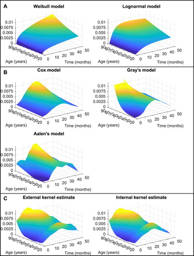
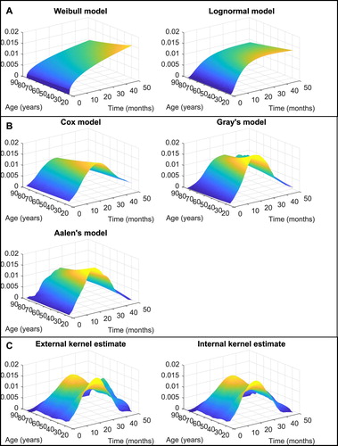
Figure 2. (A) Parametric, (B) semiparametric, and (C) kernel estimates of the conditional hazard function for triple-negative breast cancer patients treated with neoadjuvant therapy.

For the whole group, the estimate using the Weibull model shows increasing risk with time and age. The estimates of the shape and scale parameters are 0.0005 and 1.4077, respectively. The estimate of the regression coefficient of age is 0.0127, with a p-value of 0.1287. TR is 0.9910, and HR is 1.0128. Accordingly, the regression parameter is not significantly different from zero and therefore, the influence of age is not statistically relevant. However, the estimate of the regression parameter of age is $-0.01256$ with a p-value of 0.0460 using the lognormal model. Estimates of the location and scale parameters are 5.6155 and 1.2905, respectively. TR is 0.9875.

Also, semiparametric models are applied. According to Cox and Aalen's models, age is not statistically significant but is significant using Gray's model. The Cox estimate of regression parameter is 0.0126 with a p-value of 0.1269 and HR of 1.0127. The overall test for the significance of age in Aalen's model has a p-value of 0.1724. Finally, the test for the effect of age in Gray's model has a p-value of 0.0493. The estimates of the baseline hazard are similar across all semiparametric models. There is one peak at 30 months after diagnosis. Additionally, the risk of death increases with age. According to Gray's model, the influence of age is stronger in the first months after diagnosis. Note that the graph of Gray's conditional hazard function in Figure 1 is truncated due to comparability with other estimates.

Finally, external and internal kernel estimates provide a similar shape of the conditional hazard function. Unlike other estimates, the risk of death is highest for younger and older patients. Dependence on time after diagnosis is also different in these two groups. Younger patients achieve the highest risk about 25 months after diagnosis, while older patients have the greatest period of risk sooner after diagnosis.

The influence of age on the conditional hazard function is different for the neoadjuvant-treated patients. According to both parametric models, the risk of death is slightly increasing for younger patients. However, no statistical significance of regression coefficients is observed for Weibull and lognormal model ($-0.0069$, p-value 0.6201, and 0.0067, p-value 0.5282). In the Weibull model, the shape and scale parameters are 1.4223 and 0.0026, respectively. In the lognormal model, the location and scale parameters are 3.8879 and 1.0557, respectively.

Semiparametric models showed a nonsignificantly increased risk of death for the younger neoadjuvant-treated patients. The Cox estimate of regression parameter of age is $-0.0068$ with a p-value of 0.6273 and HR of 0.9932. The significance tests of the age effect have p-values of 0.5907 and 0.8454 for Aalen's and Gray's model, respectively.

Both types of kernel estimates show a high risk of death for the youngest patients but also the patients under about 50 years. This age effect is in accordance with the aggressivity of TNBC and patient selection guidelines for neoadjuvant therapy. Moreover, with longer follow-up time, the risk of older relative to younger patients increases.

Overall, the shapes of kernel estimates are closed to corresponding empirical conditional hazard function and using them may be selected a suitable parametric or semiparametric model which is easier to interpret or categorized the covariate. In the presented data, age shows a nonlinear effect on the risk of death, accordingly, categorizing could be considered.

5. Simulation study

The previous application to real data showed a significant influence of model selection on the conditional hazard estimation when interpreting the results. An incorrect choice, or simplifying assumptions, can lead to the loss of important information. The kernel estimators are more flexible in this respect. The simulation study aimed to evaluate the quality of kernel estimation for different situations. A known model was focused on, i.e. situations of known survival time distribution or the fulfilment of other assumptions. Additionally, some general situations were considered. Firstly, a 30% censoring rate was studied, then the influence of increasing the censoring rate or sample size was considered.

5.1. Structure of the simulation study and description of data generation

100 samples were simulated, each comprising 200 or 500 triples of complete data $(X_i,T_i,C_i)$ and the same number of triples of observed data $(X_i,Y_i,C_i)$ for a specified conditional hazard function $\lambda (t|x)$. The iid covariates were assumed to follow uniform distribution on the interval $(0,10)$. The iid survival times were obtained numerically by resampling the random variables $U_i$ uniformly distributed on the interval $(0,1)$, i.e. $T_i=F^{-1}(U_i|X_i),\mathrm{where}F(t|x)=1-{\mathrm{e}}^{-{\int }_0^t\lambda (u|x)}\mathrm{d}u.$The iid censoring times follow a lognormal distribution with parameters 2.5 and ${0.2}^2$, i.e. $C_i\sim \log \mathcal{N}(2.5,{0.2}^2)$ independent of the covariates and survival times. An uniform distribution of censoring times on the interval $(5,20)$ was used, but it is not referred to in this paper. See [41] for details how given censoring time distribution parameters with predefined censoring rates were determined.

The error between the true and the estimated conditional hazard function was measured by the average squared error $\mathrm{ASE}(\hat{\lambda })=\frac{1}{n}\sum _{i=1}^n{(\hat{\lambda }(Y_i|X_i)-\lambda (Y_i|X_i))}^2.$The kernel estimates were compared with parametric and semiparametric models in all simulations. Kernel smoothing was used to obtain better estimates in semiparametric models. The main idea is to use equation $\hat{\lambda }(t)=\frac{1}{h}\int K\left(\frac{t-u}{h}\right)\mathrm{d}\hat{\mathrm{\Lambda }}(u)$where a smoothed hazard is obtained from a non-parametric estimate of the cumulative hazard. This can be used to obtain ${\lambda }_0(t)$ in Cox, Gray's, and Aalen's models and the regression coefficient function $\beta (t)$ in Aalen's models.

The Epanechnikov kernel was used in all simulations. Optimal bandwidths for the external and internal kernel estimators were calculated and used in each sample [see][24]. However, obtaining optimal bandwidths for semiparametric models is not possible because the assumptions of the models are often violated. For this reason, bandwidths were selected empirically to achieve a minimum ASE. Note, however, that the effect of the smoothing parameters was not crucial with regard ASE comparison with other models.

5.2. Compared models

In this section, individual simulation cases are introduced. The conditional hazard functions with a censoring rate of 30% are summarized in Figure 3.

Figure 3. Graphs and formulas of conditional hazard functions in simulation study.

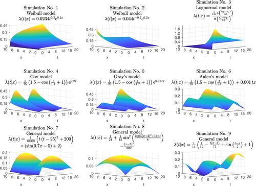
Survival times in the first simulation follow a Weibull distribution with a scale parameter of 0.018, a shape parameter of 1.3, and a regression coefficient of 0.2. The risk of death increased with time and with the value of a covariate. The second simulation is again the Weibull model but with alternative parameters, namely 0.055 and 0.8 for scale and shape parameters, respectively. The hazard function is decreasing relative to time. Conversely, the hazard function for the third simulation reached a maximum for a small covariate value and short time from the beginning. This hazard function corresponds to lognormal distribution with a zero location parameter, scale parameter of 0.5, and a regression coefficient of $\frac{1}{3}$. This is therefore the AFT model $\ln T_i=\frac{1}{3}{X}_i+{\epsilon }_i$, where ${\epsilon }_i\sim \mathcal{N}(0,{0.5}^2)$.

Simulation No. 4 to 6 have a very similar conditional hazard function. There are two peaks in the time direction and the risk of death increases with a covariate. A difference is in the shape of the dependence on the covariate values. While the case of Cox and Gray's models is an exponential dependence, a linear dependence was considered for Aalen's model. Also, this dependence is time-varying for both Gray's and Aalen's models.

The last three simulations do not correspond to any known distribution or model. In the first, the risk of death is maximum for low and high covariate values. Dependence on time has the same shape for different covariate values, increasing until it reaches a maximum and then decreasing again. This shape of the conditional hazard function was chosen based on experience from application to real data. This situation is present for cancer data where younger patients often have more aggressive tumours and therefore suffer a higher risk of death.

The second general simulation corresponds parabolic shape of the conditional hazard function. The higher risk of death is for intermediate values of the covariate. The last general simulation is more complicated. The hazard function undulates across time and the covariate, achieving maximum for low covariate values.

Note that functions in Figure 3 correspond to the 30% censoring rate. A higher censoring rate can be obtained in several ways. The first is to change the parameters of the lognormal distribution of censoring times. However, this causes shorter observed times. The conditional hazard functions will obtain different shapes and this can influence the quality of estimation methods. The effect of the censoring rate has a more complicated explanation. Thus another approach was taken. Each hazard function in Figure 3 was multiplied by a constant. Thus, different censoring rates with the same censoring time distributions are obtained. The shape of the conditional hazard is also retained. For comparability of ASEs across different censoring rates, ASEs were rescaled. Then, rescaled ASE for the multiplication of the hazard function by the constant c is $\frac{\mathrm{ASE}}{c^2}$. This approach can not be used in simulation No. 3 of the lognormal model. Therefore, simulation No. 3 was not considered for censoring rates of 60% and 90%.

5.3. Results

The results of the simulation study are summarized in Figures 4–6 for each censoring rate. Summary statistics of results can be found in Tables 1–6 of the Supplementary Material. All results are for lognormal distributed censoring times.

Figure 4. Box plots of logarithm ASE for a 30% censoring rate and the sample size of the simulated data set 200 (left box plot) and 500 (right box plot). Each figure represents one simulation of conditional hazard from Figure 3 and the estimate of the conditional hazard is performed in seven ways – Weibull, Lognormal, Cox, Gray's, Aalen's models, or external and internal types of kernel estimates. The median is always inside the box and the ends of the whiskers extend to 1.5 times the interquartile range from the box. Grey points are individual values of log ASE. The long-dashed lines correspond to the medians for the internal kernel estimates, and the dot-dashed lines are medians for the external kernel estimates.

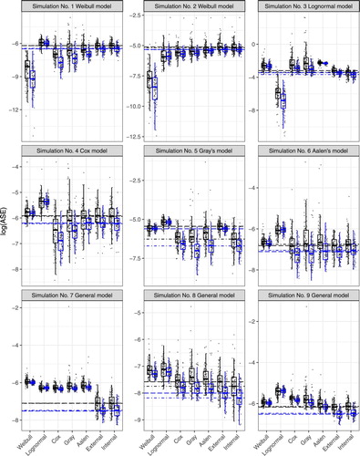
Firstly, details of the results of the study for a 30% censoring rate were dealt with. In simulations No. 1 and 2, survival times followed a Weibull distribution. The hazard ratio was also constant over time and an exponential effect of the covariate in the conditional hazard function was present. Therefore, the assumptions of Weibull, Cox, and Gray's models were satisfied. As expected, these models produced the best results. Obviously, estimates using the Weibull model were appreciably better due to satisfying stronger assumptions. In simulation No. 2, the benefit of the Weibull model is more pronounced. Also, the highest ASE values are in the lognormal model with a different survival time assumption. Both types of kernel estimates gave similar ASE values, which were slightly higher than those for semiparametric models. A similar phenomenon in the second simulation can be seen, except that the assumptions of semiparametric models were not satisfied, and the results for kernel estimates were better than using semiparametric models.

Simulations No. 4 and 5 from Cox and Gray's models have very similar results. The best estimates were produced by the models where simulated data were fully consistent with these models. Other semiparametric simulations were slightly worse, following kernel estimates. Parametric models provided the highest ASE values. The results of simulation No. 6 of Aalen's model were a bit surprising. Although the simulation data followed Aalen's model, estimates using this model were not the best. The best result was obtained using kernel estimates and the Cox model.

Finally, the simulations of general models demonstrated the benefit of kernel estimates. In these cases, survival times followed an unknown distribution, the influence of a covariate was not exponential or linear, and the hazard ratio was not constant over time. Therefore, the parametric and semiparametric models failed. Estimates of the conditional hazard function similar to the function in the application (see Figures 1–2) were considerably better using kernel estimates than others in Simulation No. 8 or 9. This difference between kernel estimates and others was not as pronounced in the last simulation, but kernel estimates still had the lowest ASE values.

Evaluation of results regards to sample size change shows consistent behaviour for greater sample size. The ASE values are lower and the differences among models are more distinct.

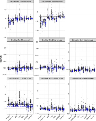
With an increasing censoring rate, ASEs increased as expected, the differences between estimates were diminished, while the relationships between estimates were mostly retained. Only in Simulation No. 9 with a 90% censoring rate were parametric models better than other estimates. The explanation of this fact will be a part of a future simulation study.

The interesting facts are also the large variability of ASE and the large number of outliers for Gray's model in most considered simulations. For this reason, the scale of y-axis in Figures 4–6 is sometimes confusing.

The simulation study was completed by repeating it with uniformly distributed censoring. The results were very similar and no fundamental differences were noticed.

Figure 5. Box plots of logarithm rescaled ASE for a 60% censoring rate and the sample size of the simulated data set 200 (left box plot) and 500 (right box plot). Each figure represents one simulation of conditional hazard from Figure 3 multiplied by a constant and the estimate of the conditional hazard is performed in seven ways – Weibull, Lognormal, Cox, Gray's, Aalen's models, or external and internal types of kernel estimates. The median is always inside the box and the ends of the whiskers extend to 1.5 times the interquartile range from the box. Grey points are individual values of log ASE. The long-dashed lines correspond to the medians for the internal kernel estimates, and the dot-dashed lines are medians for the external kernel estimates.

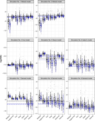
Figure 6. Box plots of logarithm rescaled ASE for a 90% censoring rate and the sample size of the simulated data set 200 (left box plot) and 500 (right box plot). Each figure represents one simulation of conditional hazard from Figure 3 multiplied by a constant and the estimate of the conditional hazard is performed in seven ways – Weibull, Lognormal, Cox, Gray's, Aalen's models, or external and internal types of kernel estimates. The median is always inside the box and the ends of the whiskers extend to 1.5 times the interquartile range from the box. Grey points are individual values of log ASE. The long-dashed lines correspond to the medians for the internal kernel estimates, and the dot-dashed lines are medians for the external kernel estimates.

The aim of this simulation study was not to compare both types of kernel estimates but to independently evaluate and compare with other methods. According to the theoretical results [see][24], both types have the same asymptotic variance, but asymptotic bias is different depending on the data. According to this simulation study, both types of kernel estimates provide similar results except Simulation No. 5. The internal type seems to be better in this case. Explanation of this behaviour can be a subject for further investigation.

Finally, note, we considered fixed bandwidths for each kernel estimate due to the time-consuming nature of bandwidths selection methods. We could obtain better results of kernel estimates by selecting more appropriate parameters for the specific sample.

6. Conclusion

In this paper, two types of kernel estimators were mentioned and subsequently compared with commonly used models using real data and the extensive simulation study. The simulation study revealed that the kernel estimator did not fail in any situation. Naturally, when data are fully consistent with the model, estimation using this model is the most advantageous. However, for real data, this situation does not occur practically. The theoretical shape of the conditional hazard function or distribution of the survival time is not known, and assumptions of semiparametric models are often violated. In these situations, kernel estimation is, therefore, a very helpful alternative.

The advantage of parametric and semiparametric models is straightforward interpretation. However, this interpretation loses its meaning when the assumptions of the models are violated (e.g. [42] discussed the impact of misspecifying fully parametric PH and AFT models). To verify these assumptions, kernel estimation can be used. Furthermore, as demonstrated by real data, it could offer possibilities to divide individuals into groups with a similar risk of death, i.e. finding thresholds of continuous variables.

Application to real data of TNBC patients showed a failure of parametric models, especially in the neoadjuvant-treated subgroup of patients. Semiparametric models were not able to capture the inconsistent risk of death in individual age groups. The effect of age could thus be nonsignificant despite possible differences. Aalen's and Gray's models were able to capture at least time-dependence age influence.

The kernel methods are able to estimate different shapes of the hazard function without limitations and smooth them out. They are able to capture any changes in the hazard function in both time and covariate directions. The disadvantages of kernel estimators can be regarded as the computational complexity of and absent standard software implementation. The kernel estimates are also influenced by bandwidths choice and care must be taken to avoid under- and oversmoothing.

The introduced two types of kernel estimators have different statistical properties, especially their asymptotic bias depending on the data distribution. However, a comparison of external and internal estimators was not the aim of this study. It deserves a more comprehensive study to identify situations when one of the types of estimates needs to be preferred.

The output of kernel estimates is not a number that could be well interpreted but a visualization of the conditional hazard function. It should not be considered to be a deficiency with respect to other non-parametric or parametric estimates because it is estimated without other restrictions. The problem arises in the case of multiple covariates. Kernel estimates are still possible, but more sophisticated visualization tools are not available for their presentation yet. It is possible to bypass it by displaying cuts of function.

In this study, in practice most commonly used right censoring independent of failure was considered. Nevertheless, this strong assumption could be violated, and alternative models could be taken into account. Parametric and semiparametric models were extended for interval censoring [see][43] or informative censoring [see][44]. Similarly, kernel estimators of hazard function were considered with alternative types of censoring [see][45–47]. The computational complexity of conditional kernel estimates exacerbated by considering different censoring is probably the reason for the lack of publication in this area.

Finally, the simulation study could be extended to consider more models. As already indicated, more attention could be given to the effect of the censoring rate. The kernel estimators could be modified, whereas their performance at boundary points differs from interior points due to boundary effects. There are two approaches to avoid this problem. The first is to use a boundary-adjusted kernel [see][48] and the second is to use asymmetric kernels [see][49,50].

Disclosure statement

No potential conflict of interest was reported by the author(s).

Additional information

Funding

This research was supported by the Ministry of Health, Czech Republic – Conceptual Development of Research Organization [grant number MMCI 00209805]; Ministry of Education, Youth and Sports, MEYS – Czech Clinical Research Infrastructure (CZECRIN) [grant number LM2018128], [grant number BBMRI–CZ LM2018125]. The work of Stanislav Katina was supported (partly) by the long-term strategic development financing of the Institute of Computer Science [grant number RVO:67985807] and specific research of Masaryk University as support for student projects [grant number MUNI/A/1615/2020].

Appendix. Methods for selection of bandwidths

A.1. Cross-validation method

The integrated squared error (ISE) is considered in the form $\mathrm{ISE}(\hat{\lambda })=\iint {(\lambda (t|x)-\hat{\lambda }(t|x))}^{2}f(t|x)s(x)\mathrm{d}x\mathrm{d}t=I_1-2I_2+I_3$where $\begin{array}{rl}{I}_1& =\iint {\hat{\lambda }}^2(t|x)f(t|x)s(x)\mathrm{d}x\mathrm{d}t,\\ I_2& =\iint \hat{\lambda }(t|x)\lambda (t|x)f(t|x)s(x)\mathrm{d}x\mathrm{d}t,\\ I_3& =\iint {\lambda }^2(t|x)f(t|x)s(x)\mathrm{d}x\mathrm{d}t.\end{array}$The aim is to minimize ISE relative to the smoothing parameters. The expression $I_3$ is not dependent on smoothing parameters and it can be left out it for these purposes. Expression $I_1$ and $I_2$ depend on unknown functions. They must be estimated from the data.

$I_2$ can be rewritten as $I_2=\iint \hat{\lambda }(t|x)\frac{r(t|x)}{\overline{L}(t|x)}f(t|x)s(x)\mathrm{d}x\mathrm{d}t.$Estimates of $I_1$ and $I_2$ using the leave-one-out principle are defined as $\begin{array}{rl}{I}_1& =\frac{1}{n}\sum _{i=1}^n\int {\hat{\lambda }}^2(t|X_i)\hat{f}(t|X_i)\mathrm{d}t,\\ I_2& =\frac{1}{n}\sum _{i=1}^n\frac{{\hat{\lambda }}_{-i}(Y_i|X_i)}{\hat{\overline{L}}(Y_i|X_i)}{\hat{f}}_{-i}(Y_i|X_i){\delta }_i,\end{array}$where ${\hat{\lambda }}_{-i}(t|x)$ is the estimate of the conditional hazard function based on the data $\{(X_j,Y_j,{\delta }_j),j\ne i\}$, $\hat{\overline{L}}(t|x)$ is the kernel estimate of the survival function of the observable time defined by (3(3) $\hat{\overline{L}}(t|x)=\sum _{i=1}^n{w}_i(x)W\left(\frac{Y_i-t}{h_t}\right).$(3) ), $\hat{f}(t|x)$ is the kernel estimate of survival density given by $\hat{f}(t|x)=\hat{\lambda }(t|x){\mathrm{e}}^{-{\int }_0^t\hat{\lambda }(u|x)\mathrm{d}u}$and ${\hat{f}}_{-i}(t|x)$ is its leave-one-out version.

The cross-validation function is defined in the form $\mathrm{CV}(h_x,h_t)=\frac{1}{n}\sum _{i=1}^n\int {\hat{\lambda }}^3(t|X_i){\mathrm{e}}^{-{\int }_0^t\hat{\lambda }(u|X_i)\mathrm{d}u}\mathrm{d}t-\frac{2}{n}\sum _{i=1}^n\frac{{\hat{\lambda }}_{-i}^2(Y_i|X_i)}{\hat{\overline{L}}(Y_i|X_i)}{\mathrm{e}}^{-{\int }_0^{Y_i}{\hat{\lambda }}_{-i}(u|X_i)\mathrm{d}u}{\delta }_i$and bandwidths are chosen to minimize this function, i.e. $({\hat{h}}_{x,\mathrm{CV}},{\hat{h}}_{t,\mathrm{CV}})=\arg \underset{(h_x,h_t)}{min}\mathrm{CV}(h_x,h_t).$Note, that the leave-one-out estimators have the forms ${\hat{\lambda }}_{-iE}(t|x)=\frac{\frac{1}{h_t}{\displaystyle \sum _{j\ne i}{w}_j(x)K\left(\frac{t-Y_j}{h_t}\right){\delta }_j}}{{\displaystyle \sum _{j\ne i}{w}_j(x)W\left(\frac{Y_j-t}{h_t}\right)}},$and ${\hat{\lambda }}_{-iI}(t|x)=\frac{1}{h_t}{\displaystyle \sum _{j\ne i}K\left(\frac{t-Y_{(j)}}{h_t}\right)\frac{{\delta }_{(j)}{w}_{(j)}(x)}{1-{\displaystyle \sum _{k=1}^{j-1}{w}_{(k)}(x)}}.}$for the external and internal estimators, respectively. In addition, weights in these estimators are based on the leave-one-out principle, too.

A.2. Maximum-likelihood method

This method is based on the conditional likelihood function and its maximization relative to the smoothing parameters. The conditional likelihood function is obtained using the conditional density of $(Y,\delta )$ given X = x, i.e. $l(t,\delta |x)$. This density can be written as $l(t,\delta |x)={[f(t|x)\overline{G}(t|x)]}^{\delta }{[g(t|x)\overline{F}(t|x)]}^{1-\delta }$due to equalities $l(t,1|x)=r(t|x)=f(t|x)\overline{G}(t|x)$ and $l(t,0|x)=g(t|x)\overline{F}(t|x)$.

Assume the distribution of censoring time is not dependent on smoothing parameters. Now, consider maximizing the likelihood as a function of $h_x$ and $h_t$ only. The function to be maximized is $\mathcal{L}(h_x,h_t)=\prod _{i=1}^n{f}^{{\delta }_i}(Y_i|X_i){\overline{F}}^{1-{\delta }_i}(Y_i|X_i)=\prod _{i=1}^n{\lambda }^{{\delta }_i}(Y_i|X_i)\overline{F}(Y_i|X_i).$This function is estimated using kernel estimation from the data. Again, the leave-one-out estimator defined previously is used. The maximum-likelihood method is then based on the modified likelihood function in the form $\mathrm{ML}(h_x,h_t)=\prod _{i=1}^n{\hat{\lambda }}_{-i}^{{\delta }_i}(Y_i|X_i){\hat{\overline{F}}}_{-i}(Y_i|X_i)$where ${\hat{\overline{F}}}_{-i}(t|x)={\mathrm{e}}^{-{\int }_0^t{\hat{\lambda }}_{-i}(u|x)\mathrm{d}u}.$Bandwidths are chosen to maximize this function, i.e. $({\hat{h}}_{x,\mathrm{ML}},{\hat{h}}_{t,\mathrm{ML}})=\arg \underset{(h_x,h_t)}{max}\mathrm{ML}(h_x,h_t).$

References

- Kaplan EI, Meier PV. Nonparametric estimation from incomplete observations. J Am Stat Assoc. 1958;53(282):457–481.
- Horová I, Koláček J, Zelinka J. Kernel smoothing in MATLAB: theory and practice of kernel smoothing. Singapore: World Scientific; 2012.
- Wand MP, Jones MC. Kernel smoothing. London: Chapman & Hall; 1994.
- Kalbfleisch JD, Prentice RL. The statistical analysis of failure time data. New York: John Wiley & Sons; 2002.
- Cox DR. Regression models and life-tables. J R Stat Soc Ser B. 1972;34(2):187–220.
- Aalen OO. A linear regression model for the analysis of life times. Stat Med. 1989;8(8):907–925.
- Kooperberg C, Stone CJ, Truong YK. Hazard regression. J Am Stat Assoc. 1995;90(429):78–94.
- Rosenberg PS. Hazard function estimation using B-splines. Biometrics. 1995;51(3):874–887.
- Watson GS, Leadbetter MR. Hazard analysis I. Biometrika. 1964;51(1/2):175–184.
- Watson GS, Leadbetter MR. Hazard analysis II. Sank Indian J Stat Ser A. 1964;26(1):101–116.
- Uzunoguallari Ü, Wang JL. A comparison of hazard rate estimators for left truncated and right censored data. Biometrika. 1992;79(2):297–310.
- Nielsen JP, Linton OB. Kernel estimation in a nonparametric marker dependent hazard model. Ann Stat. 1995;23(5):1735–1748.
- Spierdijk L. Nonparametric conditional hazard rate estimation: a local linear approach. Comput Stat Data Anal. 2008;52(5):2419–2434.
- Kim C, Oh M, Yang SJ, et al. A local linear estimation of conditional hazard function in censored data. J Kor Stat Soc. 2010;39(3):347–355.
- Tanner MA, Wong WH. The estimation of the hazard function from randomly censored data by the kernel method. Ann Stat. 1983;11(3):989–993.
- Müller HG, Wang JL. Nonparametric analysis of changes in hazard rates for censored survival data: an alternative to change-point models. Biometrika. 1990;77(2):305–314.
- Li G. Optimal rate local smoothing in a multiplicative intensity counting process model. Math Methods Stat. 1997;6(2):224–244.
- Van Keilegom I, Veraverbeke N. Hazard rate estimation in nonparametric regression with censored data. Ann Inst Stat Math. 2001;53(4):730–745.
- Linton OB, Nielsen JP, Van de Geer S. Estimating multiplicative and additive hazard functions by kernel methods. Ann Stat. 2003;31(2):464–492.
- Wolter JL. Kernel estimation of hazard functions when observations have dependent and common covariates. J Econom. 2016;193(1):1–16.
- R Core Team. R. A language and environment for statistical computing. Vienna, Austria: R Foundation for Statistical Computing; 2015. Available from: http://www.R-project.org/.
- Beran R. Nonparametric regression with randomly censored survival data. University of California at Berkeley; 1981. Technical report.
- Klein JP, Moeschberger ML. Survival analysis: techniques for censored and truncated data. New York: Springer; 2003.
- Selingerová I. Kernel estimates of hazard function (in Czech). [Dissertation]. Brno Masaryk University; 2015.
- Gámiz ML, Kulasekera KB, Limnios N, et al. Applied nonparametric statistics in reliability. London: Springer; 2011.
- Bagdonavicius V, Nikulin M. Accelerated life models: modeling and statistical analysis. Boca Raton/Florida: CRC Press; 2001.
- Wei LJ. The accelerated failure time model: a useful alternative to the Cox regression model in survival analysis. Stat Med. 1992;11(14–15):1871–1879.
- Therneau TM, Grambsch PM. Modeling survival data: extending the Cox model. New York: Springer; 2000.
- Vaida F, Xu R, et al. Proportional hazards model with random effects. Stat Med. 2000;19(24):3309–3324.
- Schemper M, Wakounig S, Heinze G. The estimation of average hazard ratios by weighted Cox regression. Stat Med. 2009;28(19):2473–2489.
- Gray RJ. Flexible methods for analyzing survival data using splines, with applications to breast cancer prognosis. J Am Stat Assoc. 1992;87(420):942–951.
- Valenta Z, Weissfeld L. Estimation of the survival function for Gray's piecewise-constant time-varying coefficients model. Stat Med. 2002;21(5):717–727.
- Aalen OO. Further results on the non-parametric linear regression model in survival analysis. Stat Med. 1993;12(17):1569–1588.
- Scheike TH, Zhang MJ. An additive–multiplicative Cox-Aalen regression model. Scand J Stat. 2002;29(1):75–88.
- Scheike TH, Zhang MJ. Extensions and applications of the Cox-Aalen survival model. Biometrics. 2003;59(4):1036–1045.
- Royston P, Parmar MK. Flexible parametric proportional-hazards and proportional-odds models for censored survival data, with application to prognostic modelling and estimation of treatment effects. Stat Med. 2002;21(15):2175–2197.
- Lambert PC, Royston P. Further development of flexible parametric models for survival analysis. Stat J. 2009;9(2):265–290.
- Talamakrouni M, Van Keilegom I, El Ghouch A. Parametrically guided nonparametric density and hazard estimation with censored data. Comput Stat Data Anal. 2016;93:308–323.
- Oueslati A, Lopez O. A proportional hazards regression model with change-points in the baseline function. Lifetime Data Anal. 2013;19:59–78.
- Svoboda M, Navrátil J, Fabian P, et al. Triple-negative breast cancer: analysis of patients diagnosed and/or treated at the Masaryk Memorial Cancer Institute between 2004 and 2009 (in czech). Klin Onkol. 2012;25(3):188–198.
- Wan F. Simulating survival data with predefined censoring rates for proportional hazards models. Stat Med. 2017;36(5):838–854.
- Hutton J, Monaghan P. Choice of parametric accelerated life and proportional hazards models for survival data: asymptotic results. Lifetime Data Anal. 2002;8(4):375–393.
- Sun J. The statistical analysis of interval-censored failure time data. New York (NY): Springer New York; 2006. Statistics for Biology and Health.
- Jackson D, White IR, Seaman S, et al. Relaxing the independent censoring assumption in the Cox proportional hazards model using multiple imputation. Stat Med. 2014;33(27):4681–4694.
- Betensky RA, Lindsey JC, Ryan LM, et al. Local EM estimation of the hazard function for interval-censored data. Biometrics. 1999;55(1):238–245.
- Rabhi Y, Asgharian M. Inference under biased sampling and right censoring for a change point in the hazard function. Bernoulli. 2017;23(4A):2720–2745.
- Scharfstein DO, Robins JM. Estimation of the failure time distribution in the presence of informative censoring. Biometrika. 2002;89(3):617–634.
- Müller HG, Wang JL. Hazard rate estimation under random censoring with varying kernels and bandwidths. Biometrics. 1994;50(1):61–76.
- Chen SX. Probability density function estimation using gamma kernels. Ann Inst Stat Math. 2000;52(3):471–480.
- Bouezmarni T, El Ghouch A, Mesfioui M. Gamma kernel estimators for density and hazard rate of right-censored data. J Probab Stat. 2011;2011: 937574.