Model fit criteria curve behaviour in class enumeration – a diagnostic tool for model (mis)specification in longitudinal mixture modelling

Abstract

The use of longitudinal finite mixture models (FMMs) to identify latent classes of individuals following similar paths of temporal development is gaining traction in applied research. However, FMM’s users may be unaware of how data features as well as the inappropriate specification of the model’s covariance structure impacts class enumeration. To elucidate this, we investigated model fit-criteria curve behaviour across an array of data conditions and covariance structures. Fit statistic patterns were variable among the fit criteria and across a range of data conditions. This variability was greatly attributable to the level of class separation and the presence/absence of random effects. Our findings support some widely held notions (e.g. BIC outperforms other criteria) while debunking others (adding random effects is not always the solution). Based on the obtained results, we present guidelines on how the behaviour of fit criteria curves can be used as a diagnostic aid during class enumeration.

KEYWORDS:

• Growth mixture model
• latent class growth analysis
• trajectory
• repeated measures
• covariance misspecification
• class extraction

1. Introduction

Longitudinal finite mixture models (FMM) are model-based clustering approaches designed to uncover latent heterogeneity in longitudinal profiles of the repeated measures type. This heterogeneity is usually represented as developmental trajectories, which comprise both inter-individual (between-subjects) and intra-individual (within-subjects) variability over time. These methods assist in identifying distinct latent classes of subjects within the population that show similar (within-class) temporal development. Assignment of subjects to such classes is typically done according to where their posterior probability (of the parameters) given the data is highest. Popular longitudinal FMMs include growth mixture models (GMM) [1], latent class growth analysis (LCGA) [2], and group-based trajectory models (GBTM) [3].

Longitudinal FMMs are increasingly used in applied sciences, particularly health sciences to understand differences in the development and aetiology of a variety of disorders and diseases, as well as subject responses to treatment. Recent studies include whether group differences in alcohol consumption are related to cardiovascular disease [4], understanding different treatment responses for adults with obsessive-compulsive disorder [5], and establishing the link between cannabis use in adolescents and a variety of health factors [6].

Nonetheless, it is often overlooked in practice that analysis results obtained with FMMs are sensitive to violations of their underlying assumptions, in particular the variance-covariance structure of the outcome variables in each class. This paper will investigate the impact of between-subject covariance misspecification on fit statistic behaviour during class extraction and, ultimately, on the choice of the number of classes. We examine, for instance, whether an inconclusive behaviour (e.g. continual improvement) of the considered model fit statistics (AIC, BIC, ssBIC and scaled entropy) as a function of increasing the number of fitted classes, a recurring phenomenon in practice [7], is evidence of such covariance misspecification. We ascertain that identified fit statistic behaviour under such misspecifications may be used as a diagnostic tool in finding an adequate covariance structure.

We conduct a simulation study in which several data features (design conditions) are manipulated (e.g. number of repeated measures, degree of class separation, trajectory shape, true covariance structure), conforming to a specific GMM, LCGA or GBTM model. We then fit models misspecified in terms of the covariance to the data to investigate (1) whether a plateauing behaviour (or other peculiar behaviour) of the fit statistics under the fitted model is a relic of covariance misspecification, (2) how sensitive in terms of class enumeration are these fit statistics to covariance misspecification under various data features (e.g. class separation, number of time points), and (3) whether identified fit statistic patterns may assist in finding the correct model. Moreover, an empirical example using alcohol consumption data is used to illustrate the fit criteria curves as a diagnostic aid during class enumeration and model specification. Such a diagnostic tool may be useful since covariance misspecification has important consequences for both class extraction and classification performance [8–14].

2. Specification of models

Longitudinal FMMs develop from the premise that within the population, K latent classes (subgroups) exist with subjects within classes following similar paths of development over time (trajectories). The marginal probability distribution $P({\mathit{y}}_i)$ of a randomly chosen trajectory is then modelled as, (1) $P({\mathit{y}}_i)=\sum _{k=1}^K{\pi }_k{P}^k({\mathit{y}}_i)$(1) where ${\mathit{y}}_i=(y_{i1},\dots ,y_{iT})$ is a vector of repeated measures for subject $i,i=1,\dots ,n$ at time $t,t=0,\dots ,T-1$, and $P^k({\mathit{y}}_i)$ is the conditional distribution of the longitudinal sequence, ${\mathit{y}}_i$, given that the subject $i$ is in class $k,k=1,\dots ,K$. Further, ${\pi }_k$ is the class membership probability and conforms to ${\pi }_k\ge 0,\sum _{k=1}^K{\pi }_k=1$, with $K>1$. These models assume K to be known, but this is difficult to deduce directly from the data.

For continuous outcomes data, $P^k({\mathit{y}}_i)$ is assumed multivariate normal (MVN) within classes, that is, (2) ${\mathit{y}}_{\mathit{i}}^{\mathit{k}}\sim \mathit{M}\mathit{V}\mathit{N}({\mathit{\mu }}^k,{\mathbf{\Sigma }}^k)$(2) with ${\mathit{y}}_{\mathit{i}}^{\mathit{k}}$ a $T\times 1$ vector of continuous outcomes for subject $i$, and ${\mathit{\mu }}^k$ and ${\mathbf{\Sigma }}^k$ are the model-implied mean vector and covariance matrix for class $k$ respectively. $P^k({\mathit{y}}_i)$ is uniquely defined by the trajectory specification per class.

A GMM is the most general of our considered longitudinal FMMs. It includes both fixed effects to quantify class specific average growth curves and random effects to allow for individual differences (inter-individual differences) from the average growth curve within classes. Its class-specific trajectories may be expressed as, (3) ${\mathit{y}}_{\mathit{i}}^{\mathit{k}}=\mathbf{\text{X}}{\mathit{\beta }}^{\mathit{k}}+\mathbf{\text{Z}}{\mathit{b}}_{\mathit{i}}^{\mathit{k}}+{\mathit{e}}_{\mathit{i}}^{\mathit{k}}$(3) where the superscript $k$ specifies the class, $\mathbf{\text{X}}$ is a $T\times b$ design matrix for the fixed effects, ${\mathit{\beta }}^k$ is a $b\times 1$ vector of fixed effects, $\mathbf{\text{Z}}$ is a $T\times q$ design matrix for the random effects, ${\mathit{b}}_{\mathit{i}}^{\mathit{k}}$ is a $q\times 1$ vector of random effects, and ${\mathit{e}}_{\mathit{i}}^{\mathit{k}}$ is a $T\times 1$ residual vector. It is assumed that ${\mathit{b}}_{\mathit{i}}^{\mathit{k}}\sim \mathit{N}(0,{\mathbf{\text{D}}}^{\mathit{k}})$ and ${\mathit{e}}_{\mathit{i}}^{\mathit{k}}\sim \mathit{N}(0,{\mathbf{\text{R}}}^{\mathit{k}})$. ${\mathbf{\text{D}}}^k$ is the model-implied $q\times q$ random effects covariance matrix (inter-individual variation) and ${\mathbf{\text{R}}}^k$ is the $T\times T$ residual covariance matrix (intra-individual variation) of the $k$-th class. Ultimately, a GMM is specified where ${\mathit{\mu }}^k=\mathbf{\text{X}}{\mathit{\beta }}^{\mathit{k}}$ and ${\mathbf{\Sigma }}^k={\mathbf{\text{R}}}^{\mathit{k}}+\mathbf{\text{Z}}{\mathbf{\text{D}}}^{\mathit{k}}{\mathbf{\text{Z}}}^{\mathrm{\prime }}$ in Eq. (2).

LCGA and GBTM are special cases of Eq. (3) in which there are no random effects i.e. $\mathbf{\text{Z}}{\mathit{b}}_{\mathit{i}}^{\mathit{k}}=0$, such that ${\mathbf{\Sigma }}^k={\mathbf{\text{R}}}^{\mathit{k}}$, with ${\mathbf{\Sigma }}^k$ diagonal [10]. Diagonal ${\mathbf{\Sigma }}^k$ implies independence between the repeated measures within a given individual. LCGA models allow for the residual variance to differ between classes and time points. The GBTM, a popular special case of the LCGA, makes the explicit assumption of the residual variance being equal for all classes and all time points i.e. ${\mathbf{\text{R}}}^{\mathit{k}}=\mathbf{\text{R}}={\sigma }^2\mathbf{\text{I}}$, where $\mathbf{\text{I}}$ is the identity matrix [3,15,16].

2.1. Class enumeration

A key outcome of FMM analysis is to identify the optimal number of classes K which adequately describe the data. Several statistical fit indices can assist in selecting K [16], a process known as class enumeration (synonymous with extraction). However, no fit statistic has yet emerged as the clear best performer [17–22]. Therefore, practitioners are often advised to use a variety of fit statistics as well as a substantive interpretation of their models during class extraction [3,23,24].

In this study, we restrict ourselves to the likelihood-based, information criterion (IC) model-fit indices most often encountered in practice (and widely available by default in most software), that is, the Akaike Information Criterion (AIC), the Bayesian Information Criterion (BIC) and sample-size adjusted BIC (ssBIC). Scaled entropy (sE), a statistic derived from entropy $E(K)$, is included as a complement to the IC indices which is customarily reported as a measure of classification certainty. Table 1 presents their equations. The first term of the AIC, BIC and ssBIC reward models for having better log-likelihoods. The second term penalizes models for lack of model parsimony. sE is scaled to be bound between zero and one [25] and is higher when models show clear classification into classes.

Table 1. Summary of fit statistic calculations.

Measure	Equation	Model selection*
AIC	$-2\log [L(K)]+2[m(K)]$	Smallest value
BIC	$-2\log [L(K)]+\log (n)[m(K)]$	Smallest value
ssBIC	$-2\log [L(K)]+\log \left({\displaystyle \frac{n+2}{24}}\right)[m(K)]$	Smallest value
sE	$1-E(K)/n\log (K)$, where $E(K)=-{\displaystyle \sum _{k=1}^K\sum _{i=1}^{n}p{p}_{ik}\log [p{p}_{ik}]\ge 0}$	Largest value

*Fit statistic calculation may differ per software.

$L(K)$: Maximum likelihood of $K$-class model. $m(K)$: Number of parameters of $K$-class model. $p{p}_{ik}$: posterior probability of subject $i$ belonging to class $k$ given the data. $E(K)$: Entropy of $K$-class model. $\log (x)$: The natural logarithm of $x$. $n$: Sample size

In an ideal situation, one would expect a clear minimum of the IC and an sE close to 1 at the true number of classes. However, in practice, these ICs often do not exhibit clear-cut behaviour (e.g. a minimum value) as a function of increasing K. For instance, a ‘plateauing’ curve is frequently observed [7] in that the IC continues to improve marginally as the fitted number of classes increases. It is to be established whether sE elicits similar behaviour. We hypothesize that such behaviour is evidence of random effect (between-subject) covariance misspecification, which can have serious consequences for class enumeration accuracy, classification performance, and model interpretability [9,10]. We ascertain whether aforesaid identified behaviour may assist in finding the correct covariance specification.

2.2. Class separation

Class separation in longitudinal FMMs typically refers to the degree of overlap between growth trajectories for latent classes [26]. This may be quantified in terms of the amount of overlap between the latent classes’ growth trajectory intercept and slope or the degree of overlap between the observed repeated measures [27].

Low class separation has been shown to play a substantial role in decreasing estimation accuracy in GMMs [22,28]. However, to date, there is no consensus on the best definition of class separation, and indeed which measure of class separation to utilize (See e.g. Nowakowska et al. [29]). As such, it is largely dependent on the researcher to decide upon given the investigation at hand [26]. This study employs the Cohen’s D (CD), which is often used to quantify effect sizes [30], as a class separation measure. We report a time-averaged version, calculated as, (4) $C{D}_{ave}=\frac{1}{T}\sum _{t=0}^{T-1}\frac{|{\mu }_{at}-{\mu }_{bt}|}{{\sigma }_t^{}}$(4) where $t=0,\dots ,T-1$ is the time point, ${\mu }_{at}$ and ${\mu }_{bt}$ is the class mean (of the observed outcome variable) at time point $t$ for class $a$ and $b$ respectively, and ${\sigma }_t^{}$ is the square root of the diagonal element of the total covariance matrix ($\mathbf{\Sigma }$) corresponding to time point $t$.

Additionally, we report the multivariate Mahalanobis distance (MD) [31], a popular class separation measure in longitudinal FMM studies [32–35]. The pairwise MD in terms of the observed repeated measures is calculated as, (5) $MD=\sqrt{{({\mathit{\mu }}^a-{\mathit{\mu }}^b)}^T{\mathbf{\Sigma }}^{-1}({\mathit{\mu }}^a-{\mathit{\mu }}^b)}$(5) where ${\mathit{\mu }}^a$ and ${\mathit{\mu }}^b$ are the mean vectors of the observed repeated measures for class $a$ and $b$ respectively, and ${\mathbf{\Sigma }}^{-1}$ corresponds to the inverse of the covariance matrix of $\mathit{y}$ which is assumed equal in both latent classes [35,36]. An MD of one and three usually reflects small and large class separation respectively found in the literature [18,32,37–39].

Lastly, we provide the overlap coefficient (OVL) [29] for class separation. We calculate this as the average over all time points of the overlap of two class distributions at each time point, (6) $OVL=\frac{1}{T}\sum _{t=0}^{T-1}\left[{\int }_{-\mathrm{\infty }}^{\mathrm{\infty }}\text{min}[f_{at}(x;{\mu }_{at},{\mathbf{\Sigma }}_{at}),f_{bt}(x;{\mu }_{bt},{\mathbf{\Sigma }}_{bt})]\text{d}x\right]$(6) where $f_{at}(x;{\mu }_{at},{\mathrm{\Sigma }}_{at})$ and $f_{bt}(x;{\mu }_{bt},{\mathrm{\Sigma }}_{bt})$ correspond to the class density function (univariate normal) at time point $t$ of class $a$ and $b$ 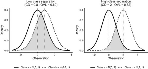respectively. Figure 1 shows low and high separation in terms of the OVL (Eq. (6)) for two univariate normal densities for a single time point. The OVL is the common area under the lower of the two density functions. The greater the overlap between the densities, the broader the $x$-axis range is where the minimum of the two densities is high. For the example of low separation, a CD of 0.8 corresponds to an OVL of 0.69 (see the grey area in the leftmost plot). For high separation, a CD of 2 results in an OVL of 0.32 (see the grey area in the rightmost plot).

Figure 1. An illustration of class separation for two univariate normal densities.

2.3. Covariance misspecification

Covariance misspecification implies assuming an incorrect structure for the random effects’ covariance matrix ${\mathbf{\text{D}}}^k$ and/or for the residual covariance matrix ${\mathbf{\text{R}}}^k$ during model estimation. Such misspecification may be broadly classified into three categories [9].

Covariance underspecification can occur when the true model includes class-specific covariance matrices (i.e. ${\mathbf{\text{D}}}^k$ and ${\mathbf{\text{R}}}^k$), but the fitted model specification constrains within-class covariance matrices to be equal across classes (i.e. ${\mathbf{\text{D}}}^k=\mathbf{\text{D}}$ or ${\mathbf{\text{R}}}^k=\mathbf{\text{R}}$) or even equal to zero (i.e. ${\mathbf{\text{D}}}^k=0$). It can also be that the true model includes equal within-class covariance matrices (i.e. ${\mathbf{\text{D}}}^k=\mathbf{\text{D}}$ and ${\mathbf{\text{R}}}^k=\mathbf{\text{R}}$), a GMM, but is specified such that ${\mathbf{\text{D}}}^k=0$, an LCGA or GBTM. Covariance overspecification can occur when the true model contains equal random effect covariance matrices across classes (i.e. ${\mathbf{\text{D}}}^k=\mathbf{\text{D}}$) or equal residual covariance matrices across classes (i.e. ${\mathbf{\text{R}}}^k=\mathbf{\text{R}}$), while the model selected for analysis allows for the estimation of class-specific matrices (i.e. ${\mathbf{\text{D}}}^k$ and/or ${\mathbf{\text{R}}}^k$). Additionally, overspecification also arises when the true model has no random effect variability within classes (i.e. ${\mathbf{\text{D}}}^k=0$) but is estimated with such variability. In this context, the true model is an LCGA or GBTM, but the assumed model is a GMM. General covariance misspecification can occur when fitting a mixture model when one is not needed, that is, where the true model consists of a single population (i.e. growth curve model), but the analysis proceeds assuming population heterogeneity (i.e. LCGA, GBTM or GMM) [9].

In our paper, we will examine the effects of under- and overspecification on fit statistic behaviour, more specifically the effect of incorrectly specifying the ${\mathbf{\text{D}}}^k$ matrix.

3. Methods

3.1. Design of the simulation study

To imitate model specifications frequently and currently used in practice [4,40–42], we limit ourselves to the case of underspecification where the true model has ${\mathbf{\text{D}}}^k=\mathbf{\text{D}}$ and ${\mathbf{\text{R}}}^k=\mathbf{\text{R}}$ (i.e. a GMM), but is estimated such that ${\mathbf{\text{D}}}^k=0$ (i.e. an LCGA or GBTM). In the case of overspecification, we investigate the impact where the true model has ${\mathbf{\text{D}}}^k=0$ with ${\mathbf{\text{R}}}^k=\mathbf{\text{R}}$ (i.e. an LCGA or GBTM), but is estimated such that ${\mathbf{\text{D}}}^k=\mathbf{\text{D}}$ (i.e. a GMM). Such equal within-class covariance matrices is the default specification of most software [16] which is often inadvertently selected by practitioners.

The (true) models for data simulation are:

• Model 1 (GBTM): With ${\mathbf{\text{D}}}^k=0$, and ${\mathbf{\text{R}}}^k=\mathbf{\text{R}}={\sigma }^2\mathbf{\text{I}}$

• Model 2 (LCGA): With ${\mathbf{\text{D}}}^k=0$, and ${\mathbf{\text{R}}}^k=\mathbf{\text{R}}={\sigma }_{{\epsilon }_t}^2\mathbf{\text{I}}$, that is, class-invariant but time-variant residual variance

• Model 3 (GMM-I): With class-invariant random intercept and random linear slope allowed to covary ${\mathbf{\text{D}}}^k=\mathbf{\text{D}}$, and ${\mathbf{\text{R}}}^k=\mathbf{\text{R}}={\sigma }^2\mathbf{\text{I}}$

• Model 4 (GMM-II): With class-invariant random intercept and random linear slope allowed to covary ${\mathbf{\text{D}}}^k=\mathbf{\text{D}}$, and ${\mathbf{\text{R}}}^k=\mathbf{\text{R}}={\sigma }_{{\epsilon }_t}^2\mathbf{\text{I}}$

We then study the effect of the chosen misspecifications by considering various fitted on true model combinations. These are shown in Table 2. The misspecification of the R matrix in terms of time-dependency (either time-variant or time-invariant) is beyond the scope of this paper, but we do note that GMM with random slopes generates heterogeneity of variance across time points and thus may resemble a time-variant in R LCGA.

Table 2. True with fitted models considered (Misspecification: a: D underspecified, b: D overspecified, c: D correctly specified).

True Model	Fitted Model
GBTM	GBTM^c	GMM-I^b
LCGA	LCGA^c	GMM-II^b
GMM-I	GMM-I^c	GBTM^a
GMM-II	GMM-II^c	LCGA^a

The design conditions underlying the data generating process are informed by previous simulation studies and applied research [13,43,44], and are summarized in Table 3 and described below.

Table 3. Primary design conditions investigated.

Design condition	Choice	Additional features
Sample size	$N=1000$
Number of repeated measures	$T=5,8$	Equally spaced
Number of classes	$K=4$
Class sizes	Equal
Class separation	Low, high	$CD=0.5,2$
Fixed effects	Same intercept and different slope (NS)	Quadratic trend
	Different intercept and different slopes (CC)
Random effects	None, or intercept and linear slope that covary	Class invariant
Errors	Time-variant or time-invariant	Uncorrelated across time, class invariant

The choice of a sample size of 1000 reflects the median condition in applied studies [44]. Furthermore, a minimum sample size of 900 is suggested under conditions of multiple classes and low class separation [45]. We also briefly investigate a sample size of 260 for a subset of models, as small sample sizes have a demonstrably negative impact on class enumeration [33], with $N=200$ being the recommended minimum for complete case data and high class separation [45].

Five repeated measures are chosen to be the lower bound at which to detect non-linear growth trajectories and to ensure model identifiability [13], especially when including full rank covariance matrices and larger $K$. This is expanded to eight to mirror the higher number of repeated measures seen in applied GMM research [33]. Moreover, it has been shown that increasing the number of time points has a positive effect on classification performance [10]. Equally spaced time values over a fixed time interval from zero to seven are chosen, and so for $T=5,t=0,1.75,3.5,5.25,7$ and for $T=8,t=0,1,2,3,4,5,6,7$. The time interval is the same for both T-values to prevent confounding of the effect of number of time points with the effect of a change of total follow-up time.

Most simulation studies in the literature consider two or three true classes. We expand upon this by including four classes. We focus primarily on equal class sizes. However, we also explore unequal class sizes $(k=1(35\text{\%})/k=2(15\text{\%})/k=3(15\text{\%})/k=4(35\text{\%}))$ for a subset of models since a substantial decrease in the class enumeration accuracy of the BIC compared to the AIC and ssBIC has been noted when one class is considerably smaller [22].

We will impose a $C{D}_{ave}$ of approximately 0.5 and 2 to reflect low and high class separation respectively. The data will be constructed in such a way that each class will be at least $C{D}_{ave}$ units away from each other. $MD$ and $OVL$ are also reported.

Fixed effects’ parameters are altered according to the degree of class separation (low or high) corresponding with our chosen Cohen’s D separation metric. We have chosen a second-order polynomial in the fixed effects as it is a flexible function which can capture many patterns across time, including monotonic trends, and u- and n-shaped trends as well as parts thereof. Two conditions of trajectory growth are studied. One in which trajectories comprise the same intercept but different slopes between classes (natural starting (NS) point) and the second includes both different intercepts and different slopes between classes. The second condition’s functional form mimics the ‘cat’s cradle’ (CC) phenomenon often identified in applied health research with a small number of time points [46–48]. Sher et al. [46] present this pattern empirically in terms of alcohol use over time. Subjects’ alcohol consumption in one class starts high and remains high (chronically bad), in a second class it starts low and remains low (unaffected/non-drinkers), in a third class it starts high but reduces over time (recovery), and in the fourth class it starts low but increases over time (delayed onset).

Lastly, we impose an $\mathbf{\text{R}}$ that is diagonal, equal across classes, and either time-variant (TV) or time-invariant (TI). For the $\mathbf{\text{R}}$ matrix of the GBTM model, each diagonal element is set to equal the average of the sum of the diagonals of the full $\mathbf{\Sigma }$ matrix of the GMM. For the LCGA specification, the diagonal elements of the $\mathbf{\text{R}}$ matrix are set equal to the corresponding diagonal elements of the $\mathbf{\Sigma }$ of the GMM. This strategy is effected so that the total average diagonal variation is similar across the design conditions. For conditions with a non-zero $\mathbf{\text{D}}$ matrix (i.e. where the true model is a GMM), the proportion of total average diagonal variation explained by the random effects was set to a fixed proportion of approximately 0.5. We enforce a weak positive correlation of 0.1 between random intercept and random linear slope, in line with previous studies [8,13,26,27,49].

The data generated are of the following general form, (7) $y_{it}^k=(b_{0i}^k+{\beta }_0^k)+(b_{1i}^k+{\beta }_1^k)t+{\beta }_2^k{t}^2+{\epsilon }_{it}^k$(7) with $k=1,..,K$, $i=1,\dots ,n$, ${\beta }_0^k,{\beta }_1^k$ and ${\beta }_2^k$ are fixed effects quantifying the population average growth curve for class $k$, and $b_{0i}^k$ and $b_{1i}^k$ are random effects that allow for individual differences from the average growth curve of class $k$. 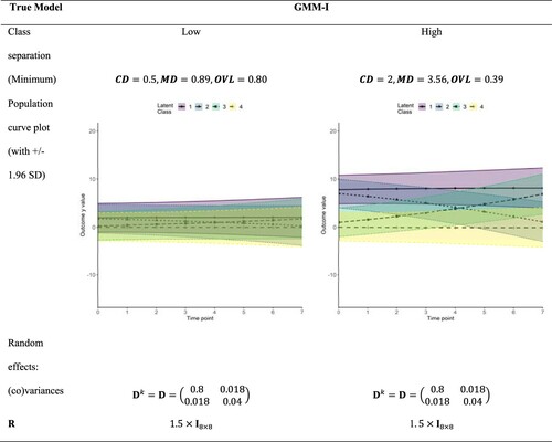In the case of LCGA and GBTM, random effects are not included. Figures 2 and 3 show the different trajectory shapes of selected true GMM-I models for different parameter sets. All considered models’ parameters are found in the supplementary material.

Figure 2. True GMM-I with NS scenario for fixed effects, $\mathit{T}=8$ and time-invariant $\mathit{R}$.

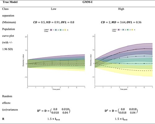
Figure 3. True GMM-I with CC scenario for fixed effects, $\mathit{T}=8$ and time-invariant $\mathit{R}$.

3.2. Simulation procedure

Longitudinal repeated measures data conforming to our true models were generated in R v3.6.3. The fitted models were estimated using the R package Mplus Automation [50], which interfaces directly with Mplus [51]. We used Mplus v7.3 for our analysis and ggplot2 in R [52] for the plotting of figures.

Subjects were first assigned to classes according to the chosen class size, e.g. for $N=1000,K=4$ and equal classes, there were exactly 250 subjects in each class. Then, a vector of random effects for each subject in a class was generated according to ${\mathit{b}}_i^k\sim MVN(0,{\mathbf{\text{D}}}^k)$. A vector of continuous repeated measures $({\mathit{y}}_i)$ for that subject within a class was then generated according to Eq. (7). This process was repeated 200 times for each of the 32 design conditions in Table 3 to generate independent datasets, giving a total of 6400 simulated datasets. Each generated dataset was used as input in the subsequent Mplus Automation step where both the true and misspecified ${\mathbf{\text{D}}}^k$ models, as given in Table 2, were fitted over $K=1,2,\dots ,10$ producing 6 400 × 2x10 = 128 000 estimated models. Anticipating that 200 replications may be too few, we ran 1000 replications for select conditions but did not observe marked differences in the results. We, therefore, adhered to 200 replications, which is in line with other published FMM research [35,53,54].

For model estimation, we bore in mind that longitudinal FMMs are notoriously sensitive to starting values for model parameters [54]. Selecting too few starting values may negatively impact the chance of finding the global solution, whilst too many may return improbable combinations, likely leading to nonconverged solutions and zero class sizes. Therefore, in line with research [13,54] and practical [51] recommendations, for a thorough investigation of the likelihood surface, we instructed Mplus to use 100 random sets of starting values for all model parameters of a given model on a given run. The programme was then ordered to run through 20 iterations on each of these sets. Next, the programme was directed to use the 10 sets yielding the highest log-likelihood from the first stage as starting values in the final stage optimization until convergence criteria were met. The model with the highest log-likelihood from this stage was used as the basis for further analysis. Any nonconverged solutions were discarded, with the proportion of non-convergence out of all 200 runs computed per design combination per true model per fitted number of classes never exceeding 5%. For 96% of the cases, nonconvergence was below 1% (See Supplement Section S.2.). If non-convergence exceeded 2%, this was always for true or fitted model GMM, T=8, low separation, and number of fitted classes exceeding 5 (See Supplement Table S.3).

4. Results

4.1. Accuracy of class extraction in relation to design conditions and D misspecification

The impact of design conditions and D misspecification on the probability of class extraction was investigated with two logistic regression analyses; one using as outcome correct versus incorrect extraction and including all cases (logistic model 1 – LM-I), and one using as outcome over- versus underextraction and including only cases of incorrect extraction (logistic model 2 – LM-II). The K chosen from the fitted models corresponded to that K at which the IC value was lowest or the sE highest. The abundance of interactions found in these analyses between true model and every other design factor in Table 3 justified separate logistic regression analyses on subsets of the data to facilitate interpretation. Subset (a) included true GMM-I and GMM-II, whilst subset (b) considered true GBTM and LCGA. These subsets corresponded to examining under- and over-specification of D respectively (See Supplementary Section S.3.1 for full logistic regression results).

In the subset analyses, two-way interactions were included to test whether the effect of D misspecification on K extraction depended on the level of the design condition (e.g. low versus high class separation) and also on the fit statistic (e.g. AIC versus BIC). Further, interactions between the fit statistic and design conditions were also considered. Likelihood ratio tests were conducted to ascertain whether the included interactions yielded a significantly better fit. Many of these interactions were significant. Of particular note were; the interactions between (1) the fit statistic and class separation across all logistic regression analyses, (2) the fitted D and fit statistic in all logistic models (except LM-II(b)), and (3) the fitted D and class separation level across all logistic models (except for LM-II (a)). These interactions are displayed in Figure 4 (to be discussed in greater detail) and Appendix Figures A.1-A.3, which show the patterns and sizes of the effects of the design conditions on class enumeration performance for each criterion.

Figure 4. Estimated probabilities of K correct (upper half) or of overextraction given incorrect K (lower half) for true by fitted model under low/high class separation given conditions: Natural starting point, T=8 repeated measures. Left half concerns models GMM-I and GBTM, right half concerns models GMM-II and LCGA.

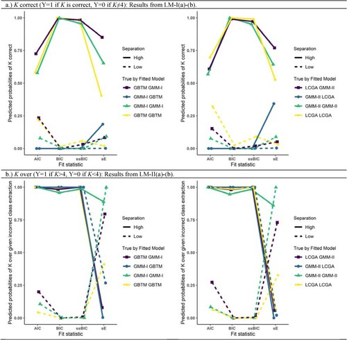
Figure 4 presents the estimated probabilities of K extraction for the fit statistics under natural starting point (NS) and eight time points (T=8) for all logistic models considered. The remaining combinations of NS/CC and T=5/T=8 are presented in the Appendix. These figures were chosen since they respect the prominent interactions of fitted D with class separation and fit statistic.

The findings of LM-I (outcome: correct class extraction) displayed in Figure 4 (a) are multifaceted. First, it shows that, irrespective of class separation, all IC fit statistics had a low probability of selecting the true K when D was underspecified (i.e. true model is GMM, fitted model is GBTM/LCGA). Further, under high class separation, BIC and ssBIC performed almost perfectly for fitted models with D overspecification (i.e. true model is GBTM/LCGA, fitted model is GMM) or correct specification, whereas the AIC and sE performed substantially worse. By contrast, all fit statistics performed poorly under low class separation irrespective of the D specification, although the AIC generally performed slightly better than the other fit statistics if D was correctly specified or overspecified. The effect of the number of time points, time-variant versus time-invariant R for all fitted models and fit statistics on correct class extraction was inconspicuous compared to the effect of class separation (See the Appendix).

Figure 4 (b) shows the results of LM-II (over- versus underextraction). Here, regardless of class separation, for underspecified D, the IC fit statistics had a 100% probability of overextraction (given incorrect extraction). For D over- or correct specification, all IC fit statistics showed a high probability to overextract under high separation and underextract under low separation. sE, however, showed converse behaviour, under- and overextracting under high and low separation respectively.

To conclude, all fit statistics performed poorly in terms of correct K extraction under low separation, with BIC and ssBIC performing the worst. Under high separation, BIC performs best, followed by the ssBIC. Furthermore, under high separation, underspecification of D is associated with a high risk of incorrect class extraction for the IC fit statistics, whereas overspecification of D for all fit statistics shows little risk of incorrect K extraction, particularly for the BIC and ssBIC. Moreover, among the cases that were incorrectly extracted, underspecification of D is associated with a high risk of overextraction by the IC statistics regardless of class separation. For over- and correct specification of D, IC fit statistics tended to overextract under high separation and underextract under low separation, among the subset of cases with incorrect extraction.

4.2. Identifiable patterns of fit statistic curves across all conditions

4.2.1. Screeplot behaviour

Each of the 32 simulation design conditions considered in Table 3 for the true model yielded fit statistic curves and summary bar charts. Given space constraints, only two of these conditions are presented in Figures 5 and 6, but the corresponding figures for all design conditions are provided in Supplement S.4. Each figure condenses the output information of 200 simulations (runs) for one design condition. For each fit criterion (rows), three distinct plots are shown (columns): the fit statistic curve given as the average over 200 runs at each number of classes (left), frequency distribution of the number of turning points of the fit statistics’ curve of a single run (middle), and frequency distribution of the final selected K (right). This information is provided in each subplot separately for each fitted model. A turning point for AIC, BIC and ssBIC is defined as a point K where $IC(K)<IC(K-1)$ and $IC(K)<IC(K+1)$. For sE this is defined as a point K where $sE(K)>sE(K-1)$ and $sE(K)>sE(K+1)$.

Figure 5. Fit statistic behaviour for true 4 class GMM-I with natural starting point, high class separation and $\mathit{T}=8$. Left column: The average fit statistic value over all runs (ordinate axis) against the number of estimated classes (abscissa); middle column: Frequency of the number of turning points in the individual fit statistic curves (n=200 runs); right column: frequency of specific K being selected.

Note: Turning point for AIC, BIC and ssBIC is defined as a point K where both $\mathit{I}\mathit{C}(\mathit{K})<\mathit{I}\mathit{C}(\mathit{K}-1)$ and $\mathit{I}\mathit{C}(\mathit{K})<\mathit{I}\mathit{C}(\mathit{K}+1)$. For sE, a turning point is defined as a point K where both $\mathit{s}\mathit{E}(\mathit{K})>\mathit{s}\mathit{E}(\mathit{K}-1)$ and $\mathit{s}\mathit{E}(\mathit{K})>\mathit{s}\mathit{E}(\mathit{K}+1)$.

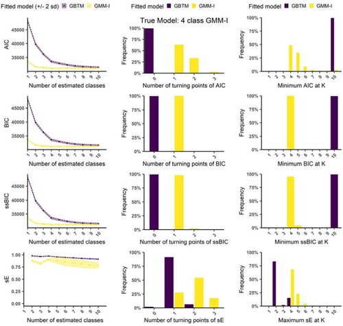
Figure 6. Fit statistic behaviour for true 4 class GBTM with natural starting point, high class separation and $\mathit{T}=8$. Left column: The average fit statistic value over all runs (ordinate axis) against the number of estimated classes (abscissa); middle column: Frequency of the number of turning points in the individual fit statistic curves (n=200 runs); right column: frequency of specific K being selected.

Note: Turning point for AIC, BIC and ssBIC is defined as a point K where both $\mathit{I}\mathit{C}(\mathit{K})<\mathit{I}\mathit{C}(\mathit{K}-1)$ and $\mathit{I}\mathit{C}(\mathit{K})<\mathit{I}\mathit{C}(\mathit{K}+1)$. For sE, a turning point is defined as a point K where both $\mathit{s}\mathit{E}(\mathit{K})>\mathit{s}\mathit{E}(\mathit{K}-1)$ and $\mathit{s}\mathit{E}(\mathit{K})>\mathit{s}\mathit{E}(\mathit{K}+1)$.

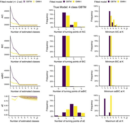
Figure 5 (true model = GMM-I) shows that when a GBTM is fitted (i.e. underspecified $\mathbf{\text{D}}$), the IC statistics exhibit clear plateauing behaviour given their continual improvement as K increases (left column). Furthermore, the general absence of turning points (middle column) highlights their proclivity to overextract as the maximum considered K=10 is always selected (right column). This conforms with the findings in Figure 4, showing the ICs’ high probability of incorrect extraction for underspecified in D models (Figure 4 (a)), see True: GMM-I Fitted: GBTM, specifically overextraction (Figure 4 (b)). This pattern is repeated throughout conditions where underspecified models are fitted (see Supplement S.4). For a correctly specified GMM, both the BIC and ssBIC are highly accurate and stable showing a large majority of one turning point at K=4. sE exhibits erratic and inaccurate performance compared to the BIC and ssBIC for the true model. AIC shows a tendency to overextract, even under the correct model. Again, these observations conform to the logistic regression results (Figure 4) which highlights the poor accuracy of the AIC and sE relative to the BIC and ssBIC.

In Figure 6 (true model = GBTM), the BIC and ssBIC of both correct and overspecified models extract the correct K. In contrast, the sE for correct D and the AIC for both correct D and overspecified D shows lower accuracy. The BIC and ssBIC do not show plateauing behaviour as there is a single turning point. This pattern recurs in similar cases (see Supplement S.4) indicating that the risk of an incorrect K under overspecification appears small with high separation.

It is noticeable that the average scree plot of the various IC fit statistics (which approximately matched the individual scree plots, one per simulated dataset) (See Supplement S.4) is smooth (i.e. gradual improvement in IC) for underspecified models, that is, when the true model is a GMM and a GBTM or LCGA is fitted. By contrast, the curves are jagged (i.e. quick uneven improvement in IC to an elbow, with no or hardly any improvement in the IC beyond the true K) for correct or overspecified models, that is, when a GBTM or LCGA is the true model underlying the data and a GBTM, LCGA or GMM is fitted. This noticeable pattern may assist practitioners in refining their model’s covariance structure as the smoothness indicates the necessity for random effects or a respecification of the covariance structure.

4.2.2. Fit statistic behaviour across all simulation conditions

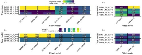
Figure 4 summarizes the results of only four of all 32 simulation conditions whilst Figures 5 and 6 do so for one condition each. Therefore, to visualize patterns within the data for all 32 simulation conditions, heatmaps [55] are presented. These heatmaps summarize the outputs of all the crossed true model by fitted model simulations for time-invariant (Figure 7) and time-variant (Appendix Figure A. 4) $\mathbf{\text{R}}$ conditions respectively. The results of the 200 simulations per design condition (rows), per fitted model and per fit criterion (columns) are summarized by two cells in separate but complementary heatmaps within Figure 7 (respectively Appendix Figure A. 4):

• each cell in panel A (for IC fit statistics) or panel C (for scaled entropy) displays the proportion of correct K extracted by the fit statistic out of all runs for each design condition,

• each cell in panel B (for IC fit statistics) or panel D (for scaled entropy) shows the modal K (i.e. the most frequent K extracted by a fit statistic) for each design condition

Figure 7. Heatmaps of the proportion correct K=4 (panels A and C) and modal K (panels B and D) extracted by different fit statistics for different fitted models under time-invariant R conditions (GBTM, GMM-I). Ordinate axis coded as H/L_NS/CC_8/5 indicating: Class separation: H(igh) or L(ow), Trajectory shape: N(atural) S(tart) or C(at’s) C(radle), and Time points: 8 or 5. All panels: Quadrants clockwise from upper left: (1) Underspecified GBTM, (2) Correctly specified GMM, (3) Overspecified GMM, (4) Correctly specified GBTM.

Combined, the two cells for a given condition inform whether the fit statistics performed well in terms of extracted K accuracy (panels A and C) under each design by fitted model condition, while simultaneously hinting at their underlying fit statistic curve behaviour (panels B and D).

Each panel is divided into 4 quadrants. The top left quadrant corresponds to underspecification of D, the bottom right quadrant represents overspecification of D, and the remaining two quadrants correspond to correct specification. Within panels, the $x$-axis corresponds to the fitted model and its associated fit statistic, e.g. GBTM (ssBIC) shows that a GBTM was fitted with its ssBIC output given. The $y$-axis shows the true model and its underlying design conditions, with the naming convention of TrueModel_Trajectory shape_Degree of class separation_Number of repeated measures. For example, the performance of the AIC for a GBTM fitted to a true GMM-I with a natural starting point and high class separation for 8 measurements (row 1 in Figure 5) corresponds to the coordinate (Panel: A and C, Row: GMM-I_NS_H(igh)_T=8, Column: GBTM(AIC)) in Figure 7. The results in the heatmaps are arranged such that the upper half of each panel corresponds to true GMM models, and the lower half to either true GBTM (Figure 7) or LCGA (Appendix Figure A. 4) models. Within each half, the results are further divided by class separation, then trajectory shape, and finally the number of repeated measures.

To facilitate interpretation, consider light cells in panel A of Figure 7. These cells have low proportions of correct K extraction. However, these cells on their own do not indicate whether the fit statistics extracted more or fewer classes than the correct K, just that K=4 was selected hardly ever in all the 200 runs. The additional nuance of under- or overextraction is found in the corresponding cell in panel B. Here, given A, if the cell in B is also light, e.g. for (GMM-I_NS_H_T=8, GBTM(AIC)) the modal K=10, this signifies class overextraction. This occurs mainly if the true model is GMM and the fitted model is GBTM, that is, if the covariance matrix D is underspecified. The fact that this overextraction is accompanied by a plateauing behaviour of the fit statistic curve is confirmed by considering both the left and middle columns of Figure 5 (or associated Supplemental figures) as discussed previously. By contrast, if the cell is light in A, but dark in B (bottom right quadrant), this is an indication of underextraction by the fit statistic i.e. the fit statistic curve reached a minimum point before the correct K. This occurs if D is correctly specified or overspecified, combined with low class separation.

Consider now the darkest cells in panel A which display the highest accuracy of correct K extracted (upper half of top right quadrant and of both bottom quadrants). Their counterparts in panel B confirm that the fit statistics excelled in selecting a modal K=4. This optimal extraction performance again transpires in exemplar Figure 6 (considering GBTM_NS_H_T=8, GBTM(BIC,ssBIC)): these IC fit statistics curve had a clear (elbow) minimum turning point at the correct K=4, with no improvement in the curve beyond the true K (left) and highest frequency of one turning point (middle).

The heatmaps thus encapsulate unfolding fit statistic patterns over increasing K, while directing attention to specific combinations of design conditions and fitted models (x- and y-axes), in which standout curve behaviours are observed.

Information criteria (IC) for time-invariant R (Figure 7A and B): What is immediately apparent is the large number of zero proportion correct K in panel A. These are seen when fitted models are underspecified in D (the upper left quadrant of panel A) or for low class separation (rows 5–8 and 13–16 from the top) independent of whether D is over-, under- or correctly specified. For high separation (rows 1–4 and 9-12), we notice with correct specification of D (upper half of upper right quadrant and of lower left quadrant of panel A) and with overspecification of D (upper half of the bottom right quadrant of panel A) high accuracy of the ICs, which in most cases exceeds 98% correct. However, the AIC is considerably less accurate than the BIC and ssBIC.

Linking the above-identified behaviour to panel B, we see that under high class separation and underspecified D this is associated with a modal K=10 in a vast majority of cases – in line with plateauing behaviour (see appendix scree and turning point bar plots) and the associated risk of overextraction. Under low class separation, underspecified D is still associated with overextraction exhibiting a high modal K where most cases exceed K=8. Therefore, when the IC of fitted GBTM selects considerably more classes than a fitted GMM, this may point to underspecification in terms of D. For high separation, the overspecified or correctly specified in D models (associated with the darker regions) show a low risk of overextraction where they almost always have a modal K at the true K. Moreover, under conditions of low separation for correctly specified and overspecified models we notice the tendency of ICs to under-extract classes.

sE for time-invariant R: sE also performs better under high class separation, but its performance is inconsistent. In particular, the sE does not appear to perform better in class extraction if the correct model is fitted than if an under- or overspecified model is fitted.

The findings of time-variant R (shown in Appendix Figure A. 4) are similar to time-invariant R. This is in line with our logistic regression results, which confirms that the effect of the level of R is small relative to those of class separation and of D specification.

To conclude, it appears that when the true model is fitted under high class separation, the best IC fit statistic is most often observed at or close to the true K showing a clear elbow. If an underspecified model, GBTM respectively LCGA, is fitted to a true GMM-I and GMM-II respectively, it is frequently observed that the AIC, BIC and ssBIC fit statistics continue to improve as K increases (plateauing behaviour). No useful fit curve behaviour for sE can be found. Lastly, fit statistic class enumeration behaves poorly under low class separation, but the patterns identified under high separation repeats in the low separation conditions, however with the modal K being lower (see Supplement S.4).

4.3. Unequal class sizes and small sample size

Whether the patterns identified above also hold for select models with unequal class sizes (two classes of 35%, two of 15%) or small sample size (N=260) was briefly investigated. Only conditions of high separation (as low separation has already been shown to be detrimental to class extraction), NS and CC, T=8 and time-invariant R, were considered.

The ICs perform similarly under unequal classes (Appendix Figure A. 5). However, compared to equal classes, the overextraction behaviour of underspecified models in D is more pronounced under unequal classes given cat’s cradle as they show a higher relative frequency of modal K=10. The BIC remains accurate with correctly specified and overspecified models. sE again performs poorly and erratically under correctly fitted models. Finally, the plateauing and elbow behaviour identified previously also holds under unequal class sizes (see Supplement S.4.3).

Under small sample conditions (Appendix Figure A. 6), the previously identified behaviour of the ICs is retained. The BIC performs better than the other ICs, but does suffer a decrease in accuracy under correctly specified GMM-I and over-specified GMM-I under CC compared to the large sample condition. We also take note of the decrease in accuracy of the ssBIC under small samples, which is noticeable given that it is meant to perform better under small samples [56]. The sE appears to perform better in small samples than in large samples, with 8/12 of the crossed models having a modal K=4 frequency of above 50%, but in general, remains an unreliable class enumeration measure. Moreover, plateauing and elbow behaviour of the IC fit statistics associated with the level of D specification is still clearly evident under small sample sizes (Supplement S.4.4).

5. Application

In this section, we will show how an appropriate covariance structure for a longitudinal finite mixture model can be selected using the fit statistic behaviour as an aid. We consider the log-transformed self-reported alcohol consumption ($A{C}_{it}^{\ast }=\text{log}(A{C}_{it}+1)$) of n=908 individuals from a former longitudinal FMM study [4]. $A{C}_{it}$ is the total volume of weekly consumption (in glasses) of subject $i$ measured at four time intervals (t = 1 Youth: 12–18 years, t = 2 Young adult: 19–27 years, t = 3 Adult: 28–44 years, t = 4 Middle age: 45–60 years). The specifications of the models fitted to the data conform to GBTM, LCGA, GMM-I and GMM-II considered in this paper. Model pairings for comparison in line with our study would be GBTM with GMM-I and LCGA with GMM-II. In line with a previous study [16], each class trajectory is modelled as a quadratic function of time, such that, (8) $A{C}_{it}^{\ast k}=({\beta }_0^k+b_{0i}^k)+(b_{1i}^k+{\beta }_1^k)tim{e}_{it}+{\beta }_2^{k}tim{e}_{it}^2+{\epsilon }_{it}^k$(8) with the specific polynomial and equation parameters conforming to Eq. (7). The objective of such an exercise is to identify classes of individuals following distinct trajectories of alcohol consumption over time.

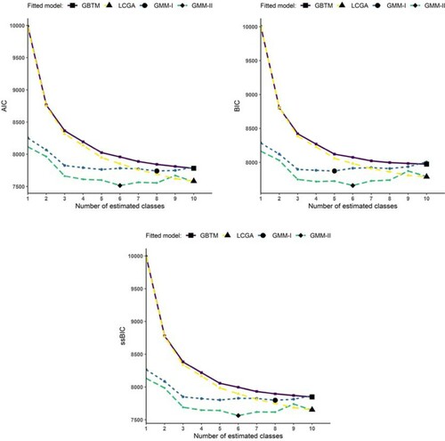
The IC fit statistic curves of the estimated models are displayed in Figure 8. We exclude sE as we have established that it exhibits no discernible pattern in identifying covariance misspecification. A plateauing behaviour of the IC statistics for the fitted GBTM and LCGA is evident, as all curves have a minimum value at K=10 (which is the maximum K examined). For the ICs, both GMM models show clear turning points at a K consistently lower than the associated GBTM or LCGA. The ICs for GMM-I suggest a K between 5 and 8 classes, whilst for GMM-II they all point to 6 classes. This preliminary evidence, taken together, hints at the LCGA and GBTM being underspecifications of the covariance structure of the data. They are, therefore, inconclusive. When presented with such fit statistic behaviour, the researcher is advised to explore models that allow for a more complex covariance structure. Accordingly, good candidate models to explore further include the GMM-I and GMM-II with their more general covariance structure. These models can then be further refined in sequential steps as has been suggested by other authors [16,24,57,58]. Such refinements would include (amongst others) inspection of models for non-convergence, non-identifiability, checking the significance of fixed effects parameters, class separation, and ascertaining distinctiveness of trajectories [16]. As an illustration, using the available OVL R code (Supplementary material), we computed the magnitude of the class separation among the K=6 trajectories (shown in the Supplement) for the GMM-II model. This yielded OVLs ranging from 0.197 (between trajectories 2 and 4) to 0.73 (between 3 and 4), indicative of high to moderately low class separation levels (See appendix).

Figure 8. Fit statistic curves of estimated models (optimum fit statistic value at bold shape).

6. Discussion

6.1. Research questions recalled

Given the above results, we can answer our research questions:

1. Is a plateauing behaviour (or other peculiar behaviour) of the fit statistics under the fitted model a relic of covariance misspecification?

We find that underspecification of the D matrix (random effects structure) across all considered design conditions leads to a continual improvement, and associated plateauing behaviour in the IC fit statistic (AIC, BIC, ssBIC) as fitted K increases. These underspecified models do not adequately capture the underlying variability (contained in D), which increases the likelihood of overextraction. This covariance misspecification is, thus, encapsulated as spurious latent classes [59]. No useful consistent pattern for sE fit curves across fitted models is easily identifiable.

1. How sensitive in terms of class enumeration are these fit statistics to covariance (D) misspecification under various data features (e.g. class separation, number of time points)?

The ICs, especially the BIC and ssBIC, of overspecified and correctly specified models enumerate accurately under high separation. The sE under similar conditions performs worse than the BIC and ssBIC. However, under low separation, all fit statistics perform poorly with the ICs tending to underextract whilst the sE overextracts. For all levels of D misspecification, the effect of the number of repeated measures, time-variant versus time-invariant R, and NS versus CC on correct K extraction by IC fit statistics is considerably lower than the effect of class separation.

1. Do identified fit statistic patterns assist in finding the correct model?

We posit that if the ICs of a fitted GBTM or LCGA continually improve as K increases, then this is indicative of covariance underspecification. This position is even more compelling if a GMM fitted to the same data yields a better fit in terms of IC fit statistics at a considerably lower K. In this case, the guidance provided by the ICs (namely the number of classes) for the GBTM or LCGA may be misleading and prone to overextraction. A thorough investigation of the proposed covariance structure and model is then warranted.

If an overspecified GMM is fitted where an LCGA or GBTM would suffice, the value of the IC fit statistics for all three fitted models tend to be lowest and similar at the true K motivating the selection of the more parsimonious (i.e. GBTM or LCGA) model. This can be confirmed using likelihood ratio tests (LRTs) [16] such as the adjusted Lo-Mendell-Rubin LRT (aLMR) [19]. Finally, no identifiable diagnostic pattern for the sE was found.

6.2. Fresh insights and recommendations

Some further insights can be gleaned from our results, which debunk, confirm and/or complement several widely held opinions about FMM class extraction:

• Firstly, although the ICs of an overspecified GMM are less likely to extract spurious classes than the ICs of an underspecified GBTM or LCGA under high separation, they, all perform poorly under low class separation. Here, the ICs of the overspecified GMM underextracts, while the ICs of the underspecified GBTM and LCGA continue to overextract, which complements established research [22,35,60]. Crucially, with low separation, the addition of random effects is not a panacea and could potentially collapse clinically meaningful classes with distinct patterns of change into a single class.

• Secondly, under high separation, the AIC shows a greater tendency to incorrectly extract classes (compared to BIC and ssBIC), even under correctly specified models. The BIC was the most accurate class enumeration fit statistic, followed by the ssBIC, but as with AIC, they tend to overextract when D is underspecified. Under low separation, all fit statistics perform poorly.

• Thirdly, the use of sE for model selection during class enumeration has been cautioned against [61]. Our findings warrant this cautionary tone.

• Fourthly, the notion that the risk of overextraction is high in particular for larger samples (N>1000) [9,21,48,53] is not fully correct. We have shown that underspecification of D can lead to overextraction even for smaller sample sizes (N=260).

Additionally, it must be emphasized that the fit statistic criteria only serve as a guide in determining the number of classes. The final decision of how many classes to extract is not an automatic process and demands considerable involvement from the researcher at every step of model fitting. This includes the judicious use of statistical analysis and substantive interpretation [24,57]. Considering our research findings, we recommend that:

• If a plateauing behaviour of ICs for GBTM and LCGA is evident, a visual inspection of the estimated mean trajectories within each class is warranted (particularly if practitioners do not have access to GMM capable software). Higher K solutions showing classes not substantively different from each other (e.g. trajectories that are either parallel, have especially low class separation, or exhibit very small or null class sizes) should be discarded and a more parsimonious model selected. Example code for OVLs, i.e. the class separation index, is provided in the supplementary material. Researchers are advised to compute the OVLs among the trajectories as an adjunct to assess the quality of class extraction.

• If there are multiple candidates for K based on the BIC, then likelihood ratio tests such as the adjusted Lo-Mendell-Rubin LRT (aLMR), substantive interpretation and visual inspection of trajectories could assist in further refining K [16,24,57,58].

• In scenarios suggesting underextraction, in particular under low-class separation, researchers are advised to carefully evaluate the distinctiveness of the longitudinal profiles of candidate models, while considering their theoretical relevance. One could check for multimodality or a wide mode of the residual distribution per time point (for GBTM), or of the random effect distribution of the intercept and slope (for GMM), with deviations from normality being indicative of possible underextraction. Failure to address this may lead to wrong inferences such as an incorrect standard error of the class trajectory slope and the slope itself may be biased. We have, however, not explored this possibility in this paper.

6.3. Class enumeration: reification and validation

In empirical sciences, FMMs are widely used for clustering purposes. Lesser known is that FMMs can be used to approximate oddly shaped distributions using a mixture of normal distributions, with specific applications in handling non-normal data including missing values [62,63] and outlier detection [64]. In a clustering context, however, this ability to approximate a non-normal distribution becomes a liability. In 2003, Bauer and Curran [49] drew attention to this by demonstrating that FMMs uncover spurious latent classes in one-class, non-normal data. Since then, other studies have replicated GMMs’ over-extracting tendency [65] within a clustering context, with a solution for that developed and implemented using robust non-normal skewed distributions [66–68]. We did not address models’ and fit criteria’ performances under violations of distributional assumptions, and further simulations should explore whether our findings can be replicated under such circumstances.

Moreover, the vicissitudes of class enumeration make the ‘reification fallacy’ [69] admonition as relevant as ever. The caution that one should refrain from interpreting latent classes as true entities, particularly in exploratory studies, is seldom misplaced. However, this issue pertains more to the external (as against internal) validation of the classes. For instance, two recent developments in FMMs applications substantiate a more theoretically founded interpretation of identified trajectories, specifically through criterion validity (genotyping) [70,71] or replicability of findings (meta-analyses) [72]. In these cases, a more lenient posture towards classes’ reification may be justified.

6.4. Limitations

We acknowledge the limitations of this study, which includes the focus on continuous repeated measures as encapsulated by a multivariate normal link function (as in Eq. (2)). It would be instructive to investigate such emergent fit statistic patterns for different data types (e.g. count and binary data). Parameter recovery of the extracted trajectories when the correct K is selected was not considered as our focus was on establishing fit statistic curve behaviour under different D misspecification. However, preliminary visual inspection of the trajectories when the known simulated K is selected (under high separation, correct and overspecified D) suggests that the recovery of trajectories’ temporal paths and class sizes is sound.

7. Conclusion

This paper has shown via extensive simulation that fit statistic curve behaviour can be a valuable diagnostic tool assisting model selection. Hence, practitioners of longitudinal FMM are advised to plot and inspect the fit statistics’ patterns of change as a function of increasing K during class enumeration. These plots engender a better understanding of data features which underlie problematic behaviour of model fit statistical indices, helping to identify possible covariance misspecification. Notably, a continual improvement of the IC for fitted GBTM and LCGA as the researcher increases the number of classes is a clear indication of the models not adequately capturing the underlying covariance structure (underspecification), which then manifests into spurious latent classes. As a tool, these plots represent an additional step in following a transparent and methodological approach when fitting longitudinal FMM [3,16,24,57].

Finally, the OVL may serve an ancillary role in model fitting by first establishing the level of class separation between extracted trajectories, and thus the quality of class extraction before further refinements in the model fitting process. For cases of low separated classes, researchers will need to go beyond fit criteria to transparently substantiate their choices, such as using complementary criteria (e.g. theoretical justification, residual plots).

Software acknowledgements

Additional packages not previously cited but used to conduct our research includes; brglm2 [73], dplyr [74], ggeffects [75], lme4 [76], stargazer [77], viridis [78].

Disclosure statement

No potential conflict of interest was reported by the author(s).

Appendix

Figure A1. Estimated probabilities of K correct (upper half) or of overextraction given incorrect K (lower half) for true by fitted model under low/high class separation given conditions: Cat’s cradle, T=5 repeated measures. Left half concerns models GMM-I and GBTM, right half concerns models GMM-II and LCGA.

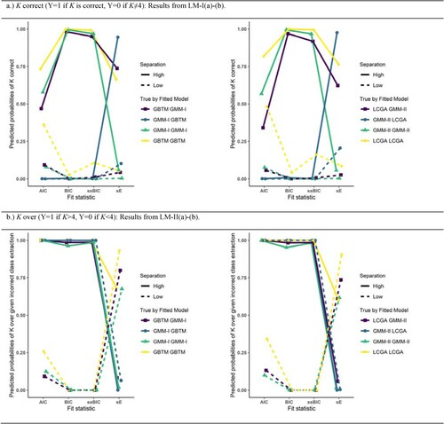
Figure A2. Estimated probabilities of K correct (upper half) or of overextraction given incorrect K (lower half) for true by fitted model under low/high class separation given conditions: Natural starting point, T=5 repeated measures. Left half concerns models GMM-I and GBTM, right half concerns models GMM-II and LCGA.

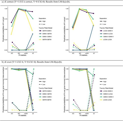
Figure A3. Estimated probabilities of K correct (upper half) or of overextraction given incorrect K (lower half) for true by fitted model under low/high class separation given conditions: Cat’s cradle, T=8 repeated measures. Left half concerns models GMM-I and GBTM, right half concerns models GMM-II and LCGA.

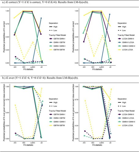
Table A1. OVL for 6-class GMM-II. Each cell corresponds to the OVL between corresponding classes given in row and column headings.

Class	k=2	k=3	k=4	k=5	k=6
k=1	0.68	0.291	0.29	0.664	0.676
k=2		0.316	0.197	0.495	0.394
k=3			0.73	0.582	0.585
k=4				0.519	0.532
k=5					0.514

Figure A4. Heatmaps of the proportion correct K=4 (panels A and C) and modal K (panels B and D) extracted by different fit statistics for different fitted models under time-variant R conditions (LCGA, GMM-II). Ordinate axis coded as H/L_NS/CC_8/5 indicating: Class separation: H(igh) or L(ow), Trajectory shape: N(atural) S(tart) or C(at’s) C(radle), and Time points: 8 or 5. All panels: Quadrants clockwise from upper left: (1) Underspecified LCGA (2) Correctly specified GMM (3) Overspecified GMM (4) Correctly specified LCGA.

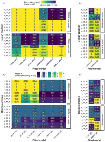
Figure A5. Heatmaps of the proportion correct K=4 (panels A and C) and modal K (panels B and D) extracted by different fit statistics for time-invariant R with unequal class sizes (35%/15%/15%/35%) (GBTM, GMM-I). Ordinate axis coded as GMM-I/GBTM_NS/CC_H/L_NS/CC_T=8/5 indicating: True Model: GMM-I or GBTM, Trajectory shape: N(atural) S(tart) or C(at’s) C(radle), Class separation: H(igh) or L(ow), and Time points: 8 or 5. All panels: Quadrants clockwise from upper left: (1) Underspecified GBTM, (2) Correctly specified GMM, (3) Overspecified GMM, 4.) Correctly specified GBTM.

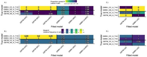
Figure A6. Heatmaps of the proportion correct K=4 (panels A and C) and modal K (panels B and D) extracted by different fit statistics for time-invariant R for N=260 (GBTM, GMM-I). Ordinate axis coded as GMM-I/GBTM_NS/CC_H/L_NS/CC_T=8/5 indicating: True Model: GMM-I or GBTM, Trajectory shape: N(atural) S(tart) or C(at’s) C(radle), Class separation: H(igh) or L(ow), and Time points: 8 or 5. All panels: Quadrants clockwise from upper left: (1) Underspecified GBTM, (2) Correctly specified GMM, (3) Overspecified GMM, (4) Correctly specified GBTM.

References

- Muthén BO, Shedden K, Muthén B, et al. Finite mixture modeling with mixture outcomes using the EM algorithm. Biometrics. 1999;55:463–469. Available from: https://onlinelibrary.wiley.com/doi/pdf/https://doi.org/10.1111/j.0006-341X.1999.00463.x.
- Berlin KS, Parra GR, Williams NA. An introduction to latent variable mixture modeling (part 2): longitudinal latent class growth analysis and growth mixture models. J Pediatr Psychol. 2014;39:188–203. Available from: https://academic.oup.com/jpepsy/article-lookup/doi/https://doi.org/10.1093/jpepsy/jst084.
- Nagin DS. Group-based modeling of development. Cambridge (MA): Harvard University Press; 2005. Available from: http://www.degruyter.com/view/books/9780674041318/9780674041318/9780674041318.xml.
- Lima Passos V, Klijn S, van Zandvoort K, et al. At the heart of the problem - a person-centred, developmental perspective on the link between alcohol consumption and cardio-vascular events. Int J Cardiol. 2017;232:304–314. Available from: https://doi.org/http://doi.org/10.1016/j.ijcard.2016.12.094.
- Falkenstein MJ, Nota JA, Krompinger JW, et al. Empirically-derived response trajectories of intensive residential treatment in obsessive-compulsive disorder: a growth mixture modeling approach. J Affect Disord. 2019;245:827–833. Available from: https://linkinghub.elsevier.com/retrieve/pii/S0165032718314083.
- Grevenstein D, Kröninger-Jungaberle H. Two patterns of cannabis use among adolescents: results of a 10-year prospective study using a growth mixture model. Subst Abus. 2015;36:85–89. Available from: http://www.tandfonline.com/doi/abs/https://doi.org/10.1080/08897077.2013.879978.
- Erosheva EA, Matsueda RL, Telesca D. Breaking bad: two decades of life-course data analysis in criminology, developmental psychology, and beyond. Annu Rev Stat Its Appl. 2014;1:301–332. Available from: http://www.annualreviews.org/doi/https://doi.org/10.1146/annurev-statistics-022513-115701.
- Enders CK, Tofighi D. The impact of misspecifying class-specific residual variances in growth mixture models. Struct Equ Model. 2008;15:75–95.
- Diallo TMO, Morin AJS, Lu HZ. Impact of misspecifications of the latent variance–covariance and residual matrices on the class enumeration accuracy of growth mixture models. Struct Equ Model. 2016;23:507–531. Available from: http://www.tandfonline.com/doi/full/https://doi.org/10.1080/10705511.2016.1169188.
- Davies CE, Glonek GFV, Giles LC. The impact of covariance misspecification in group-based trajectory models for longitudinal data with non-stationary covariance structure. Stat Methods Med Res. 2017;26:1982–1991. Available from: http://journals.sagepub.com/doi/https://doi.org/10.1177/0962280215598806.
- Morin AJS, Maïano C, Nagengast B, et al. General growth mixture analysis of adolescents’ developmental trajectories of anxiety: the impact of untested invariance assumptions on substantive interpretations. Struct Equ Model A Multidiscip J. 2011;18:613–648. Available from: http://www.tandfonline.com/doi/abs/https://doi.org/10.1080/10705511.2011.607714.
- Sijbrandij JJ, Hoekstra T, Almansa J, et al. Identification of developmental trajectory classes: comparing three latent class methods using simulated and real data. Adv Life Course Res. 2019;42:100288. Available from: https://linkinghub.elsevier.com/retrieve/pii/S1040260818301898.
- McNeish D, Harring JR. The effect of model misspecification on Growth Mixture Model class enumeration. J Classif. 2017;34:223–248. Available from: http://link.springer.com/https://doi.org/10.1007/s00357-017-9233-y.
- Sijbrandij JJ, Hoekstra T, Almansa J, et al. Variance constraints strongly influenced model performance in growth mixture modeling: a simulation and empirical study. BMC Med Res Methodol. 2020;20:276. Available from: https://bmcmedresmethodol.biomedcentral.com/articles/https://doi.org/10.1186/s12874-020-01154-0.
- Nagin DS, Land KC. Age, criminal careers, and population heterogeneity: specification and estimation of a nonparametric, mixed poisson model. Criminology. 1993;31:327–362.
- van der Nest G, Lima Passos V, Candel MJJM, et al. An overview of mixture modelling for latent evolutions in longitudinal data: modelling approaches, fit statistics and software. Adv Life Course Res. 2020;43:100323. Available from: https://linkinghub.elsevier.com/retrieve/pii/S1040260819301881.
- Brame R, Nagin DS, Wasserman L. Exploring some analytical characteristics of finite mixture models. J Quant Criminol. 2006;22:31–59. Available from: http://link.springer.com/https://doi.org/10.1007/s10940-005-9001-8.
- Kim ES, Wang Y. Class enumeration and parameter recovery of growth mixture modeling and second-order growth mixture modeling in the presence of measurement noninvariance between latent classes. Front Psychol. 2017;8, Available from: http://journal.frontiersin.org/article/https://doi.org/10.3389/fpsyg.2017.01499/full.
- Lo Y, Mendell NR, Rubin DB. Testing the number of components in a normal mixture. Biometrika. 2001;88:767–778.
- Muthén BO. Statistical and substantive checking in growth mixture modeling: comment on Bauer and Curran (2003). Psychol Methods. 2003;8:369–377. Available from: http://doi.apa.org/getdoi.cfm?doi=https://doi.org/10.1037/1082-989X.8.3.369.
- Nylund KL, Asparouhov T, Muthén BO. Deciding on the number of classes in latent class analysis and growth mixture modeling: a Monte Carlo simulation study. Struct Equ Model A Multidiscip J. 2007;14:535–569. Available from: https://www.tandfonline.com/doi/full/https://doi.org/10.1080/10705510701575396.
- Tofighi D, Enders CK. Identifying the correct number of classes in growth mixture models. In: Hancock GR, Samuelsen KM, editors. Adv latent var mix model. Greenwich (CT): Information Age; 2008. p. 317–341.
- Grimm KJ, Mazza GL, Davoudzadeh P. Model selection in finite mixture models: a k -fold cross-validation approach. Struct Equ Model A Multidiscip J. 2017;24:246–256. Available from: https://doi.org/http://doi.org/10.1080/10705511.2016.1250638.
- van de Schoot R, Sijbrandij M, Winter SD, et al. The GRoLTS-checklist: guidelines for reporting on latent trajectory studies. Struct Equ Model. 2017;24:451–467. Available from: https://doi.org/http://doi.org/10.1080/10705511.2016.1247646.
- Celeux G, Soromenho G. An entropy criterion for assessing the number of clusters in a mixture model. J Classif. 1996;13:195–212. Available from: http://link.springer.com/https://doi.org/10.1007/BF01246098.
- Depaoli S. Mixture class recovery in GMM under varying degrees of class separation: frequentist versus Bayesian estimation. Psychol Methods. 2013;18:186–219. Available from: http://doi.apa.org/getdoi.cfm?doi=https://doi.org/10.1037/a0031609.
- Tolvanen A. hideLatent growth mixture modeling: a simulation study [Internet]. Unpublishe. University of Jyvaskyla, Finland; 2007. Available from: http://urn.fi/URN:ISBN:951-39-2971-8.
- Li M, Harring JR. Investigating approaches to estimating covariate effects in growth mixture modeling: a simulation study. Educ Psychol Meas. 2017;77:766–791. Available from: http://journals.sagepub.com/doi/https://doi.org/10.1177/0013164416653789.
- Nowakowska E, Koronacki J, Lipovetsky S. Tractable Measure of Component Overlap for Gaussian Mixture Models. 2014;1–24. Available from: http://arxiv.org/abs/1407.7172.
- Cohen J. Statistical power analysis for the behavioral sciences. 2nd ed Hillsdale (NJ): Lawrence Erlbaum Associates; 1988.
- McLachlan GJ. Mahalanobis distance. Resonance. 1999;4:20–26. Available from: https://link.springer.com/content/pdf/https://doi.org/10.1007/BF02834632.pdf.
- Lubke G, Neale MC. Distinguishing between latent classes and continuous factors: resolution by maximum likelihood? Multivariate Behav Res. 2006;41:499–532. Available from: http://www.tandfonline.com/doi/abs/https://doi.org/10.1207/s15327906mbr4104_4.
- Diallo TMO, Morin AJS, Lu HZ. Performance of growth mixture models in the presence of time-varying covariates. Behav Res Methods. 2017;49:1951–1965. Available from: https://doi.org/http://doi.org/10.3758/s13428-016-0823-0.
- Martin DP, von Oertzen T. Growth mixture models outperform simpler clustering algorithms when Detecting longitudinal heterogeneity, even with small sample sizes. Struct Equ Model A Multidiscip J. 2015;22:264–275. Available from: https://doi.org/http://doi.org/10.1080/10705511.2014.936340.
- Peugh J, Fan X. How well does growth mixture modeling identify heterogeneous growth trajectories? A simulation study examining GMM’s performance characteristics. Struct Equ Model A Multidiscip J. 2012;19:204–226. Available from: http://www.tandfonline.com/doi/abs/https://doi.org/10.1080/10705511.2012.659618.
- McLachlan G, Peel D. Finite mixture models [Internet]. Wiley Ser. Probab. Stat. Appl. Probab. Stat. Sect. Hoboken, NJ, USA: John Wiley & Sons, Inc.; 2000. Available from: http://doi.wiley.com/https://doi.org/10.1002/0471721182.
- Tueller S, Lubke G. Evaluation of structural equation mixture models: parameter estimates and correct class assignment. Struct Equ Model A Multidiscip J. 2010;17:165–192. Available from: http://www.tandfonline.com/doi/abs/https://doi.org/10.1080/10705511003659318.
- He J, Fan X. Evaluating the performance of the K-fold cross-validation approach for model selection in growth mixture modeling. Struct Equ Model. 2018; 00:1–14. Available from: https://doi.org/https://doi.org/10.1080/10705511.2018.1500140.
- Liu Y, Luo F, Liu H. Factors of piecewise growth mixture model: distance and pattern. Acta Psychol Sin. 2014;46:1400. Available from: http://pub.chinasciencejournal.com/article/getArticleRedirect.action?doiCode=https://doi.org/10.3724/SP.J.1041.2014.01400.
- Mattsson M, Maher GM, Boland F, et al. Group-based trajectory modelling for BMI trajectories in childhood: a systematic review. Obes Rev. 2019;20:998–1015. Available from: https://onlinelibrary.wiley.com/doi/abs/https://doi.org/10.1111/obr.12842.
- Watson L, Belcher J, Nicholls E, et al. Latent class growth analysis of gout flare trajectories: a three-year prospective cohort study in primary care. Arthritis Rheumatol. 2020;72:1928–1935. Available from: https://onlinelibrary.wiley.com/doi/https://doi.org/10.1002/art.41476.
- Coyne SM, Padilla-Walker LM, Holmgren HG, et al. Instagrowth: a longitudinal growth mixture model of social media time Use across adolescence. J Res Adolesc. 2019;29:897–907.
- Hu J, Leite WL, Gao M. An evaluation of the use of covariates to assist in class enumeration in linear growth mixture modeling. Behav Res Methods. 2017;49:1179–1190. Available from: http://link.springer.com/https://doi.org/10.3758/s13428-016-0778-1.
- Morgan GB, Hodge KJ, Baggett AR. Latent profile analysis with nonnormal mixtures: a Monte Carlo examination of model selection using fit indices. Comput Stat Data Anal. 2016;93:146–161. Available from: https://linkinghub.elsevier.com/retrieve/pii/S0167947315000602.
- Kim SY. Sample size requirements in single- and multiphase growth mixture models: a Monte Carlo Simulation study. Struct Equ Model. 2012;19:457–476.
- Sher KJ, Jackson KM, Steinley D. Alcohol Use trajectories and the ubiquitous Cat’s cradle: cause for concern? J Abnorm Psychol. 2011;120:322–335.
- Bonanno GA. Loss, trauma, and human resilience: have we underestimated the human capacity to thrive after extremely aversive events? Am Psychol. 2004;59:20–28. Available from: http://doi.apa.org/getdoi.cfm?doi=https://doi.org/10.1037/0003-066X.59.1.20.
- McNeish D, Harring J. Covariance pattern mixture models: eliminating random effects to improve convergence and performance. Behav Res Methods. 2019. Available from: http://link.springer.com/https://doi.org/10.3758/s13428-019-01292-4.
- Bauer DJ, Curran PJ. Distributional assumptions of growth mixture models: implications for overextraction of latent trajectory classes. Psychol Methods. 2003;8:338–363. Available from: http://doi.apa.org/getdoi.cfm?doi=https://doi.org/10.1037/1082-989X.8.3.338.
- Hallquist MN, Wiley JF. Mplusautomation : an R Package for Facilitating Large-Scale LateNT VARIable analyses in M plus. Struct Equ Model A Multidiscip J. 2018;25:621–638. Available from: https://www.tandfonline.com/doi/full/https://doi.org/10.1080/10705511.2017.1402334.
- Muthén LK, Muthén BO. MPlus user’s guide. eighth Edi. Los Angeles (CA): Muthén & Muthén; 2017.
- Wickham H. ggplot2: elegant graphics for data analysis. New York: Springer-Verlag; 2016. Available from: https://ggplot2.tidyverse.org.
- Li L, Hser Y-I. On inclusion of covariates for class enumeration of growth mixture models. Multivariate Behav Res. 2011;46:266–302. Available from: http://www.tandfonline.com/doi/abs/https://doi.org/10.1080/00273171.2011.556549.
- Hipp JR, Bauer DJ. Local solutions in the estimation of growth mixture models. Psychol Methods. 2006;11:36–53. Available from: http://doi.apa.org/getdoi.cfm?doi=https://doi.org/10.1037/1082-989X.11.1.36.
- Engle S, Whalen S, Joshi A, et al. Unboxing cluster heatmaps. BMC Bioinformatics. 2017;18:63. Available from: http://bmcbioinformatics.biomedcentral.com/articles/https://doi.org/10.1186/s12859-016-1442-6.
- Henson JM, Reise SP, Kim KH. Detecting mixtures from structural model differences using latent variable mixture modeling: a comparison of relative model fit statistics. Struct Equ Model. 2007;14:202–226.
- Lennon H, Kelly S, Sperrin M, et al. Framework to construct and interpret latent class trajectory modelling. BMJ Open. 2018;8:e020683. Available from: http://bmjopen.bmj.com/.
- Ram N, Grimm KJ. Methods and measures: growth mixture modeling: a method for identifying differences in longitudinal change among unobserved groups. Int J Behav Dev. 2009;33:565–576. Available from: http://www.ncbi.nlm.nih.gov/pmc/articles/PMC3718544/pdf/nihms482397.pdf.
- Kreuter F, Muthén BO. Analyzing criminal trajectory profiles: bridging multilevel and group-based approaches using growth mixture modeling. J. Quant. Criminol. 2008.
- Lubke G, Muthén BO. Performance of factor mixture models as a function of model size, covariate effects, and class-specific parameters. Struct Equ Model A Multidiscip J. 2007;14:26–47. Available from: http://www.leaonline.com/doi/abs/https://doi.org/10.1207/s15328007sem1401_2.
- Masyn KE. Latent class analysis and finite mixture modeling. In: Little TD, editor. Oxford handb quant methods. 2013;2:784.
- Dodge HH, Shen C, Ganguli M. Application of the pattern-mixture latent trajectory model in an epidemiological study with non-ignorable missingness. J Data Sci. 2008;6:247–259. Available from: http://www.ncbi.nlm.nih.gov/pubmed/20401339.
- Little RJA. Pattern-mixture models for multivariate incomplete data. J Am Stat Assoc. 1993;88:125. Available from: https://www.jstor.org/stable/2290705?origin=crossref.
- Bouguessa M. A mixture model-based combination approach for outlier detection. Int J Artif Intell Tools. 2014;23:1460021. Available from: https://www.worldscientific.com/doi/abs/https://doi.org/10.1142/S0218213014600215.
- Guerra-Peña K, Steinley D. Extracting spurious latent classes in growth mixture modeling with nonnormal errors. Educ Psychol Meas. 2016;76:933–953. Available from: http://journals.sagepub.com/doi/https://doi.org/10.1177/0013164416633735.
- Depaoli S, Winter SD, Lai K, et al. Implementing continuous non-normal skewed distributions in latent growth mixture modeling: an assessment of specification errors and class enumeration. Multivariate Behav Res. 2019;54:795–821. Available from: https://www.tandfonline.com/doi/full/https://doi.org/10.1080/00273171.2019.1593813.
- Nam Y, Hong S. Growth mixture modeling with nonnormal distributions: implications for data transformation. Educ Psychol Meas. 2021;81:698–727. Available from: http://journals.sagepub.com/doi/https://doi.org/10.1177/0013164420976773.
- Elmer J, Jones BL, Nagin DS. Using the beta distribution in group-based trajectory models. BMC Med Res Methodol. 2018;18:152. Available from: https://bmcmedresmethodol.biomedcentral.com/articles/https://doi.org/10.1186/s12874-018-0620-9.
- Nagin DS, Tremblay RE. Developmental trajectory groups: fact or fiction? Criminology. 2005;43:873–904.
- Lubke GH, Miller PJ, Verhulst B, et al. A powerful phenotype for gene-finding studies derived from trajectory analyses of symptoms of anxiety and depression between age seven and 18. Am J Med Genet Part B Neuropsychiatr Genet. 2016;171:948–957. Available from: https://onlinelibrary.wiley.com/doi/https://doi.org/10.1002/ajmg.b.32375.
- Hall TO, Stanaway IB, Carrell DS, et al. Unfolding of hidden white blood cell count phenotypes for gene discovery using latent class mixed modeling. Genes Immun. 2019;20:555–565. Available from: http://www.nature.com/articles/s41435-018-0051-y.
- De Rubeis V, Andreacchi AT, Sharpe I, et al. Group-based trajectory modeling of body mass index and body size over the life course: a scoping review. Obes Sci Pract. 2021;7:100–128. Available from: https://onlinelibrary.wiley.com/doi/https://doi.org/10.1002/osp4.456.
- Kosmidis I. brglm2: bias reduction in generalized linear models [Internet]. 2020. Available from: https://cran.r-project.org/package=brglm2.
- Wickham H, François R, Henry L, et al. dplyr: a grammar of data manipulation [Internet]. 2020. Available from: https://cran.r-project.org/package=dplyr.
- Lüdecke D. Ggeffects: tidy data frames of marginal effects from regression models. J Open Source Softw. 2018;3:772. Available from: http://joss.theoj.org/papers/https://doi.org/10.21105/joss.00772.
- Bates D, Mächler M, Bolker B, et al. Fitting linear mixed-effects models using lme4. J Stat Softw. 2015;67, Available from: http://www.jstatsoft.org/v67/i01/.
- Hlavac M. stargazer: well-formatted regression and summary statistics tables [Internet]. Bratislava, Slovakia: Central European Labour Studies Institute (CELSI); 2018. Available from: https://cran.r-project.org/package=stargazer.
- Garnier S. viridis: default color maps from “matplotlib” [Internet]. 2018. Available from: https://cran.r-project.org/package=viridis.