Robust ranking by ensembling of diverse models and assessment metrics

Abstract

We propose an ensemble of classification models formed using different assessment metrics. For a given metric, a classifier performs feature selection and combines models based on different subsets of feature variables which we call phalanxes. This first step, which employs the algorithm of phalanx formation, identifies strong and diverse subsets of feature variables. A second phase of ensembling aggregates classifiers across diverse assessment metrics. The proposed method is applied to protein homology data to mine homologous proteins, where the feature variables used for developing classifiers are various measures of similarity scores of proteins, and found robust for ranking both evolutionary close and distant homologous proteins.

Keywords:

• Machine learning
• classification and clustering
• data mining
• feature selection
• robustness

1. Introduction

Ranking rare-class items in a highly unbalanced two-class problem is common in data mining and knowledge discovery [1–5]. Examples include finding fraudulent activities in credit card transactions [6,7], intrusion detection in internet surveillance [8–12], detection of terrorist attacks or threats [13–15], searching information on the world wide web [16–19], and ranking drug-candidate biomolecules in a chemical library [20–22].

In data mining, when the class of interest is rare, metrics of prediction accuracy need to go beyond minimizing misclassification error or maximizing accuracy [23,24]. For example, consider a dataset containing 1000 objects out of which 5 belong to the rare class. A naive classifier that predicts all the objects are from the majority class would therefore achieve a $0.5\mathrm{\%}$ misclassification rate or $99.5\mathrm{\%}$ accuracy when in practice it has no power to identify the rare class instances. Therefore, instead of minimizing misclassification rate, we evaluate a classifier by its ability to rank the rare class objects such that the rare class instances appear at the top of a ranked list [25,26]. The object with the largest probability has rank 1, and the object with the second largest probability has rank 2, and so on. There are several ways to assess the quality of a ranked list of the rare class instances, detailed in Section 2, leading to different metrics for building models and evaluating them.

The different metrics focus on diverse aspects of a ranked list of the rare class instances. Some metrics are heavily focused on performance at the beginning of the list: Are the top-ranked candidates actually rare class instances? Success at the beginning of the list is more likely for the rare class instances that are easy-to-spot as measured by the feature variables and assessment metrics [27,28]. In contrast, another metric – called rank last – records the position in the list of the last true rare class instance. Optimization of rank last helps a better ranking of the difficult-to-spot rare class instances [26,29]. Thus, aggregating the ensemble of phalanxes (EPX) [22,30] models across the diverse metrics aims to achieve good ranking performance for all the rare class instances, whether they are easy or difficult to spot. The results in Section 5 show that it is possible to find a single robust ensemble that performs well, to rank rare class instances, according to all measures.

Several machine learning methods have been applied to detect rare class items in binary classification problems, such as hidden Markov models [31], support vector machines (SVMs) and neural networks [32], and Markov random fields [33]. Yen and Lee [34] proposed an under-sampling method for the majority class objects to improve classification accuracy for the minority class objects in several imbalanced class distribution problems. Liu et al. (2017) [35] introduced a novel method for over-sampling minority class examples with application to medical data relating Glioblastoma patient survival. These methods are based on one trained model only and are not ensembles of classifiers.

Ensemble methods that combine multiple models are generally considered more powerful for any prediction problem [36–40]. In a binary classification problem, Chawla et al. (2003) [41] presented a novel approach for learning from imbalanced datasets, based on a combination of the synthetic minority over-sampling technique (SMOTE) algorithm and the boosting [39] procedure, where the latter is an ensemble method. The method of weighted random forests [42], which assigns large and small weights to the minority and majority class instances, respectively, is motivated by applications with imbalanced data. Lin and Nguyen [43] alleviated the data imbalance problem in a boosting ensemble via a hybrid-sampling method involving oversampling and undersampling to decrease the amount of data in majority classes and increase the amount of data in minority classes.

It is well recognized that ensembling is the most effective when diverse models are combined [36,38,44–46]. Popular methods for creating diversity are random perturbation of the training data possibly combined with random perturbation or clustering of the feature variables [22,30,36,38,47–49], or random projections of subsets of the feature variables [40,50]. In this article, we introduce statistical diversity by ensembling several logistic-regression models based on diverse and disjoint subsets of feature variables called phalanxes [22,30,49], which makes use of high-dimensional features even when the response data are sparse. As an analogy for the usefulness of diverse subsets of features, in the case of credit card frauds [6,7], there could be some who are rather blunt and relatively easy to spot by models based on some subsets of features versus others who are more sophisticated and better exposed by models based on other subsets of features. In this article, in addition to statistical diversity based on subsets of features, further diversity is created by building different ensembles of phalanxes for each of several assessment metrics (see Section 2.5).

First, for a given metric, following the idea presented in [22,30], we construct an ensemble of phalanxes (EPX). Phalanxes are disjoint subsets of features chosen in a data-adaptive way using the metric in an objective function. One classifier is fit to each phalanx, and their various estimates of the probability for the rare class are averaged for an EPX classifier. Second, different metrics in phalanx formation lead to different EPX models; their probability estimates are again averaged in an ensemble of metrics (EOM). We call the overall classifier an ensemble of phalanxes and metrics EPX-EOM. We are unaware of any previous work on injecting diversity into ensembles through a variety of evaluation objectives, especially of the ranking for the rare class instances. The advantages of these multiple levels of diversity in statistical modelling results in the detection of a wider range of rare class instances (see Section 5.4).

The proposed methodology has been applied to the problem of ranking homology status of proteins. Two or more proteins are homologous if they share a common evolutionary origin or ancestry. Understanding homology status helps scientists to infer evolutionary sequences of proteins [51,52]. It is also important in bioinformatics [53,54], with widespread applications in prediction of a protein's function, 3D structure, and evolution [55–61]. In protein homology, some homologous proteins are easy and difficult to rank correctly, and hence appear well up and down the ranked list, because they are ‘close’ and ‘remote’ with respect to their native proteins. There is interest in mining both types of proteins to infer functions of uncharacterized proteins and improve genomic annotations [53,62–64]. Moreover, the collection of different kinds of homologous sequences contains important information about the structure and function of unknown proteins [65]. Our proposed method has been found robust in ranking both easy-to-spot ‘close’ homologues and difficult-to-spot ‘distant’ homologues.

In short, the objectives of this paper are: (i) proposing a novel procedure for building ensembles of diverse models to mine a minority class of instances (e.g. homologous proteins) which are rare and challenging to detect, and (ii) discovering novel knowledge as to how and why ensembling across diverse evaluation metrics helps to achieve robust ranking of the rare class of instances.

The rest of the article is organized as follows. Section 2 defines three evaluation metrics specific to ranking rare class instances and illustrates how their diverse characteristics are potentially helpful for developing methodology. Section 3 describes the algorithm for the construction of an ensemble of phalanxes: how to find phalanxes of variables to serve in base logistic-regression models and how both phalanxes and complementary evaluation metrics are used in an overall ranking ensemble to detect rare class items. Section 4 describes the protein homology data and the feature variables available for developing the classifiers. Section 5 showcases the results of the ensemble and makes comparisons with multiple winners of the KDD Cup competitions (completed and ongoing) and other state-of-the-art ensembles (random forests, ensemble of phalanxes using random forests). Finally, Section 6 discusses the results and draws conclusion.

2. Assessment metrics for mining rare class and their diversity

We present the ranking problem as follows. Let Y be the response variable, taking value 1 for the rare class and 0 otherwise. Let $\mathbf{x}=(x_1,\dots ,x_d{)}^T$ be the set of feature variables used for developing models to estimate the probability $\pi (\mathbf{x})$ that Y = 1, that is, $\pi (\mathbf{x})=E(Y\mid \mathbf{x})$. We build our model using training data for which y and $\mathbf{x}$ are both known. The trained model is then used to predict the unknown class status y in a test set for which only $\mathbf{x}$ is known. The performance of a model is then assessed in terms of how well the estimated probabilities for the rare class in a list of objects place the rare class objects ahead of the majority class objects. After providing some visual intuition, we describe three metrics to measure specific ranking properties of a ranked list, to be used for training an algorithm and assessment.

2.1. Hit curves

We visualize the overall ranking performance of a classifier using a hit curve. Suppose that the n cases in a test set are ranked by a classifier to have nonincreasing estimated probability for the rare class. Let h be the number of rare class objects to be found in the test set, and among the top t ranked objects let $h_t\in \{0,1,2,\dots ,min(h,t)\}$ be the number of rare class objects or ‘hits’ found. The plot of $h_t$ against t for the n test cases is called a hit curve. For example, Figure 1(a) illustrates three hit curves of a particular dataset of n = 861 objects, of which h = 50 belong to the rare class. Hit curve A is uniformly better than hit curve B, as $h_t^A\ge h_t^B$ for every $t\in \{1,\dots ,n\}$. On the other hand, a classifier C with a hit curve close to the diagonal line shows performance similar to random ranking. Ideally, we want hit curves that demonstrate an initial maximal slope of 1 hit per candidate until all the hits are exhausted.

Figure 1. Example hit curves. Panel (a) shows curves A, B and C. Hit curve A is superior to B, while C has performance only comparable with random ranking. In panel (b) hit curves D and E cross each other at several locations making their comparison more difficult.

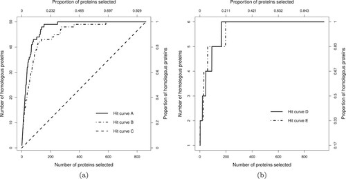
Hit curves are difficult to optimize numerically as they are hard to characterize by a unique scalar objective. Sometimes they cross each other, making comparison even more difficult. For instance, Figure 1(b) shows hit curves D and E for another dataset with n = 949 and h = 6. The curves cross at several points, and hence neither is uniformly superior. Using several numerical summaries of a hit curve provides an opportunity to ensemble classification models trained for different ranking aspects of a curve. We used three evaluation metrics to assess the ranking performance of a hit curve for which the definitions are described next.

2.2. Average precision

Average precision (APR) is a variant of the metric average hit rate [66], and its application is common in information retrieval [19]. If there are $h_t$ ‘hits’ (rare class objects) among the first t ranked objects, then $h_t/t\in [0,1]$ is the precision (or hit rate) computed at t. Let $1\le t_1<t_2<\cdots <t_h\le n$ be the positions in the ranked list where the h rare class objects are found. Then APR is defined as (1) $\mathrm{APR}=\frac{1}{h}(\frac{1}{t_1}+\frac{2}{t_2}+\cdots +\frac{h}{t_h}).$(1) APR averages ‘precisions’ at the ranking positions of the rare class objects. It considers the ranking of rare class objects in the entire test set and is similar to the area under the ROC curve. A larger APR value implies better predictive ranking, with the maximum 1 reached if and only if all of the rare class objects appear at the beginning of the list, i.e. $j=t_j$ for all $j=1,\dots ,h$ in Equation (1(1) $\mathrm{APR}=\frac{1}{h}(\frac{1}{t_1}+\frac{2}{t_2}+\cdots +\frac{h}{t_h}).$(1) ). APR is highly influenced by the ranking performance at the beginning of the list. For instance, if the first hit is found in the second versus first positions, its contribution to APR is halved from $(1/h)(1/1)$ to $(1/h)(1/2)$.

2.3. Rank last

As the name implies, the metric rank last (RKL) is the position of the last rare class object found in the entire ranked list. Therefore, it is a measure of worst-case ranking accuracy, and smaller values are better. Ties are treated conservatively: if the last ranked rare class object is in a group of objects with tied probabilities, the last member of the tied group determines the RKL. Therefore, RKL is always at least h, and the maximum possible value is the size of the dataset.

2.4. TOP1

If the top-ranked candidate is a rare class object, TOP1 scores 1 for success, otherwise, it is 0. TOP1 is calculated conservatively when there are ties: if the largest estimated probability occurs multiple times, all the objects in the tied group must belong to the rare class to score 1; any majority class object in the tied group leads to a TOP1 score of 0. Therefore, it is never beneficial to have tied probabilities. The goal is to maximize TOP1.

2.5. Diversity in assessment metrics

The following toy example illustrates how the three assessment metrics are complementary to each other in terms of ranking rare class objects: Some metrics are good for easy-to-spot rare class objects and others are good for difficult-to-spot rare class objects. Table 1 shows APR, RKL, and TOP1 from five classifiers ranking two rare class objects in a large number of objects.

Table 1. A toy example showing complementary ranking behaviour of the evaluation metrics.

	Ranks of the		Metrics
Classifier	rare objects		APR	RKL	TOP1
1	1	2	1	2	1
2	1	20	0.55	20	1
3	2	4	0.50	4	0
4	8	200	0.0675	200	0
5	10	50	0.0070	50	0

Classifier 1 ranks both of the rare class objects at the head of the list and is therefore optimal according to all evaluation metrics. Classifiers 2 and 3 have similar APR scores because classifier 2 obtains a large APR contribution from the rare class object ranked 1, which more than offsets the relatively poor rank of 20 for the second rare class object. Similarly, TOP1 favours classifier 2 over 3, but RKL gives a large penalty to classifier 2 because the second rare class object is not found until position 20. Rows 4 and 5 show much weaker classifiers. TOP1 cannot separate these classifiers, and they have similarly poor APR scores. Their RKL values better reflect the weaker worst-case ranking performance of classifier 4, however, which does not find the second rare class object until position 200 in the ranked list. We also note from this example that APR and TOP1 both give considerable weight to the head of the ranked list, but the very discrete TOP1 fails to separate the fairly good performance of classifier 3 from the much poorer performances of classifiers 4 and 5. Even though the metrics TOP1 and RKL seem trivial, they along with APR provide important information for the different kinds of rare class objects in the ranked list of objects.

3. Method of ensembling across phalanxes and assessment metrics

We describe the two levels of ensembling, first across phalanxes of features for a fixed assessment metric, and then across assessment metrics.

3.1. Ensemble of phalanx formation

The method for hierarchical clustering of features into phalanxes is adapted from [22,30]. For a fixed assessment metric, the algorithm of phalanx formation generates a set of phalanxes, where the feature variables in a phalanx will give one prediction model for mining rare homologous proteins, and those models are ensembled. See Algorithm 1 for the algorithm of phalanx formation maximizing an assessment metric a. While the algorithm of phalanx formation minimizing an assessment metric r is reported in the appendix (Algorithm 2), we next provide rationale for the adaptations.

3.1.1. Base classifier: logistic regression

The algorithm of phalanx formation chooses subsets of feature variables to be used by a base classifier. Thus there is flexibility to choose a base classifier that performs well for the given application. A submission to the KDD Cup by the research group [67] predicted the same protein-homology data fairly well using logistic regression (LR). Their preliminary analysis used feature selection to LR, which is not necessary here as the step-wise construction of candidate phalanxes and their final screening provides implicit feature selection. Another advantage of LR is that it is computationally much faster than RF and many other classification methods. As well as improving predictive ranking performance with reduced computational burden, the use of LR demonstrates that EPX is adaptable to a base learner other than the previously used RF.

3.1.2. Cross-validation instead of out-of-bag

The clusters of feature variables (phalanxes) were chosen using cross-validated probabilities obtained from the training data. To evaluate predictive ranking performance of an LR model for the training data, throughout we use the same 10-fold cross-validation (CV). Note that the use of CV is necessary here as RF's out-of-bag option does not apply to LR.

3.1.3. Criterion for merging groups of feature variables

Let a be an assessment metric (larger the better predictive ranking for definiteness), and at any iteration of phalanx formation let ${\mathbf{g}}_i$ for $i=1,\dots ,s$ be a group of the feature variables. Initially, each ${\mathbf{g}}_i$ contains one of the available feature variable.

Consider two distinct groups ${\mathbf{g}}_i$ and ${\mathbf{g}}_j$; their two LR models have metric values $a_i$ and $a_j$, respectively. If the groups are merged, their single LR model gives $a_{ij}$ for the metric, whereas ensembling (i.e. averaging probabilities for the rare class) their two respective LR models gives $a_{\overline{ij}}$. To avoid degrading the performance of a group of important feature variables by merging it with another containing less useful feature variables, our criterion for merging combines the two groups that minimize $m_{ij}=\frac{max(a_{\overline{ij}},a_i,a_j)}{a_{ij}}$over all possible pairs i and j. If $a_{ij}>max(a_{\overline{ij}},a_i,a_j)$, the performance of the new single model using the union of the feature variables is better than their ensemble performance, i.e. (2) $a_{ij}>a_{\overline{ij}}$(2) and better than the individual performances, i.e. (3) $a_{ij}>a_i\mathrm{and}{a}_{ij}>a_j.$(3) When both Equation (2(2) $a_{ij}>a_{\overline{ij}}$(2) ) and Equation (3(3) $a_{ij}>a_i\mathrm{and}{a}_{ij}>a_j.$(3) ) hold, $m_{ij}$ is less than 1 and the groups of feature variables ${\mathbf{g}}_i$ and ${\mathbf{g}}_j$ are merged together. After each merge, the number of groups s is reduced by 1, and one of the new groups is the union of two old groups. The algorithm of [30] minimizes $m_{ij}=a_{\overline{ij}}/a_{ij}$, thus taking account of Equation (2(2) $a_{ij}>a_{\overline{ij}}$(2) ) but not Equation (3(3) $a_{ij}>a_i\mathrm{and}{a}_{ij}>a_j.$(3) ).

The algorithm continues until $m_{ij}\ge 1$ for all i, j, suggesting that merging either degrades individual performances or ensembling performance for mining rare class objects. At completion, s and the ${\mathbf{g}}_i$ define c = s candidate phalanxes of feature variables ${\mathbf{x}}_i={\mathbf{g}}_i$ for $i=1,\dots ,c$, to pass to the next step.

3.1.4. Criterion for filtering the candidate phalanxes

Our algorithm identifies candidate phalanxes that help all other phalanxes in the final ensemble; other candidate phalanxes are filtered out. To detect weak and harmful phalanxes, the following criterion is minimized (4) $f_{ij}=\frac{a_{\overline{ij}}}{max(a_i,a_j)}$(4) over all possible pairs of candidate phalanxes ${\mathbf{x}}_i$ and ${\mathbf{x}}_j$. If $a_{\overline{ij}}<max(a_i,a_j)$, the ensembling performance of candidate phalanxes ${\mathbf{x}}_i$ and ${\mathbf{x}}_j$ is weaker than that of the better performing individual phalanx. Equality of $a_{\overline{ij}}$ and $max(a_i,a_j)$ shows that the ensemble of the two does not improve upon individual performances. In these cases, $f_{ij}\le 1$ and the weaker phalanx among ${\mathbf{x}}_i$ and ${\mathbf{x}}_j$ (with smaller a) is filtered out. After filtering out the weaker phalanx, the number of candidate phalanxes c is reduced by 1, and the algorithm iterates until $f_{ij}>1$ (i.e. ensembling across ${\mathbf{x}}_i$ and ${\mathbf{x}}_j$ improves over individual phalaxes) or c = 1 (i.e. there is only one phalanx). Such filtering always retains the strongest among the candidate phalanxes, and all p phalanxes in the final set $\{{\mathbf{x}}_{(1)},{\mathbf{x}}_{(2)},\dots ,{\mathbf{x}}_{(p)}\}$ help each other for the overall ensembling performance.

The previous algorithm of [30] keeps a candidate phalanx in the final ensemble if the phalanx is strong by itself or strong in an ensemble with any other phalanx. The old algorithm is vulnerable to including phalanxes that are strong individually but harmful to other phalanxes in the ensemble. Such weaknesses are avoided by the new criterion set by Equation (4(4) $f_{ij}=\frac{a_{\overline{ij}}}{max(a_i,a_j)}$(4) ).

3.2. Ensembling across phalanxes

Let $\hat{\pi }({\mathbf{x}}_{(i)})$ be the vector of probabilities for the test objects obtained from an LR applied to the phalanx ${\mathbf{x}}_{(i)}$. The overall vector for the ensemble of phalanxes (EPX) is the following (5) ${\hat{\pi }}_{\mathrm{EPX}}=\frac{\hat{\pi }({\mathbf{x}}_{(1)})+\hat{\pi }({\mathbf{x}}_{(2)})+\cdots +\hat{\pi }({\mathbf{x}}_{(p)})}{p},$(5) which is used to compute assessment metrics to measure the performance of EPX for ranking rare class objects.

3.3. Ensembling across phalanxes and assessment metrics

Let ${\hat{\pi }}_{\mathrm{EPX},m}$ be the probability vector obtained from an ensemble of phalanxes (EPX) optimized on metric m of M metrics. Here, M – the number of diverse evaluation metrics to ensemble – is application dependent. We exploit the diversity in M assessment metrics to construct our proposed overall probability vector from an ensemble of phalanxes and metrics (EPX-EOM) as follows: (6) ${\hat{\pi }}_{\mathrm{EPX}-\mathrm{EOM}}=\frac{\sum _{m=1}^M{\hat{\pi }}_{\mathrm{EPX},m}}{M}.$(6) A schematic diagram of the proposed methodology for the ensemble of phalanxes and metrics (EPX-EOM) is shown in Figure 2. The aggregation across phalanxes and assessment metrics leads to results with novel knowledge and important implications. The ranking from EPX-EOM will be assessed in Section 5 along with the rankings of EPX models for individual metrics.

Figure 2. Given an assessment metric, d feature variables are formed into p phalanxes to be used into an ensemble of phalanxes. The M ensemble of phalanxes, one for each assessment metrics, are then aggregated across assessment metrics into an ensemble of phalanxes and metrics (EPX-EOM).

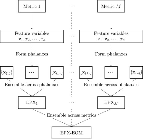
For the protein homology application below, we consider APR and RKL, hence M = 2. TOP1 is evaluated in Section 5 but not used in the ensemble of metrics; as noted in Section 2.5, APR provides better training discrimination of ranking performance at the beginning of the list.

4. Application

In our protein homology application, the proteins are either homologous or not, hence ranking of homologous proteins is a binary classification problem. Furthermore, homologous proteins are rare, and predictive ranking of a rare class is often called detection [22,30,66]. Evolutionarily related homologous proteins have similar amino-acid sequences, 3D structures and functions. Therefore, the feature variables $x_1,\dots ,x_d$ available for ranking of homology status are based on similarity scores between a candidate protein and the target native protein [68].

The protein homology dataset is downloaded from the knowledge discovery and data mining (KDD) cup competition website .¹ Registration is required to download the data and submit predictions for test proteins where only the feature variables are known. The site reports back the performance measures for ranking homologous proteins for the test data.

The dataset is organized in blocks, where the proteins in a block relate to one native protein. In total, there are 303 blocks randomly divided into training and test sets with 153 and 150 blocks/native proteins, respectively. The minimum, first quartile, median, third quartile and maximum block sizes are 612, 859, 962, 1048 and 1244, respectively, in the training set and 251, 847, 954, 1034 and 1232 in the test set.

The response variable $y\in \{0,1\}$ is 1 if a candidate protein is homologous to the block's native protein, and 0 otherwise. The homology status is known for the 145,751 proteins in the training set and unknown for the 139,658 proteins in the test set. The training dataset contains very few homologous proteins relative to non-homologous proteins. For example, the minimum, first quartile, median, third quartile and maximum of the within-block proportions of homologous proteins in the training dataset are 0.00080, 0.00143, 0.00470, 0.01206 and 0.05807, respectively. More than $75\mathrm{\%}$ of the blocks in the training set contain at most 2 homologous proteins per 100 candidates.

The 74 continuous feature variables available in the training and test sets for developing classifiers represent similarity scores of amino acid sequences between a native protein and a candidate protein. The feature variables include measures of global and local sequence alignment, global and local structural fold similarity (protein threading), position-specific scoring and profile (PSI-BLAST), and so forth. The description of the feature variables is available at the KDD cup competition website², and Teodorescu et al. (2004) [69] and the appendix of Vallat et al. (2008) [70] provide further details. The KDD Cup feature variables are still central in ongoing methodological advances for homology detection [71]. Vyas et al. (2012) [72] reviewed recent advances in homology modelling and discussed their role in predicting protein structure with various applications at the different stages of drug design and discovery. Makigaki and Ishida (2020) [73] and Senior et al. (2020) [74] show the fundamental importance of developing machine learning models to predict protein homology.

This KDD Cup dataset has also been used as a benchmark for homology modelling for other objectives. Bachem et al. (2015, 2018) [75,76] and Hirschberger et al. (2019) [77] used the data to illustrate new methods for clustering of proteins. Tsai et al. (2016) [78] also used these data to demonstrate the performances of distributed computing and cloud computing methods.

The winner for the ranking of rare homologous proteins in the 2004 knowledge discovery and data mining (KDD Cup) competition was the Weka Group [79]. They tried a large number of classifiers and selected the top three classifiers: $(1)$ a boosting ensemble [80] of 10 unpruned decision trees, $(2)$ a linear support vector machine (SVM) [81] with a logistic model fitted to the raw outputs for improved probabilities, and $(3)$ ${10}^5$ or more random rules, a variant of random forests (RF) [38]. The top three classifiers, where two are already ensemble methods, were aggregated to obtain the winning ensemble.

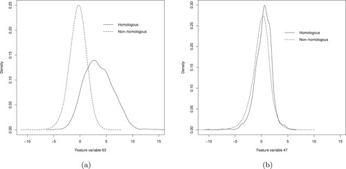
Some of the feature variables are potentially helpful for classification. For instance, Figure 3(a) shows density plots of feature variable 63 in the training data, conditioned on homology status. This variable seems to differentiate the homologous and non-homologous classes of proteins fairly well. In contrast, Figure 3(b) shows analogous density plots for feature variable 47, where the two classes are not well separated. The presence of less-informative feature variables justifies the use of feature selection we described in Section 3.

Figure 3. Density plots of the feature variables 63 (panel a) and 47 (panel b) for the homologous (solid line) and non-homologous proteins (dashed line) in the training data.

5. Results

In the training set, a native protein has an associated block of proteins with known homology status. As homologous proteins are rare in the candidate set for a single native protein, we combine training data across all native proteins to build a classifier. The classifier is then tested on a new set of native proteins, each with its own block of proteins to rank the rare class. Three metrics are used to assess the ranking performance of a model. As the data come in blocks, each of the three metrics is computed in each block separately. Given a metric, the average performance across the blocks is used as the final value of the metric. Therefore, in order to perform well, a classifier has to rank the rare homologous proteins well across many blocks.

We first present summaries for ensembles fit the protein homology training data. EPX ensembles are built separately for the APR and RKL metrics and then combined in an overall ensemble of phalanxes across the two assessment metrics. Their performances on the test set are then compared.

5.1. EPX optimized for APR

Row 1 of Table 2 summarizes the phalanxes (subsets of diverse feature variables) formed by optimizing APR. None of the 74 feature variables are filtered out in the first stage of the algorithm, hence all belong to one of the five candidate phalanxes found. Two candidate phalanxes are filtered out at the final stage, with the surviving three phalanxes containing 36, 23 and 5 variables, respectively, i.e. a total of 64 feature variables.

Table 2. Number of candidate and filtered phalanxes identified by EPX and the sizes of the filtered phalanxes.

	Number of phalanxes
Metric	Candidate	Filtered	Filtered-phalanx sizes
APR	5	3	36, 23, 5
RKL	7	2	29, 27

Note: The training data are used to optimize either APR or RKL.

A comparison of training (from CV) and test APRs is shown in Table 3. The second column shows 10-fold CV APRs for the three LR models fitted to the three phalanxes and for their EPX-APR ensemble. Here, CV is defined at the block level: the 153 blocks in the training data are randomly divided into 10 folds, where each fold contains the data from around 15 blocks. After fitting a phalanx's LR using 9/10 of the training folds, estimated probabilities of homology are obtained for the remaining hold-out fold as usual in CV. Repeating this process 10 times produces estimated probabilities for all the training data.

Table 3. Training (10-fold CV) and test set APRs for each of the three EPX phalanxes of feature variables found by maximizing APR and for the EPX-APR ensemble.

	APR
Phalanx	Training (CV)	Test
1	0.794	0.800
2	0.785	0.783
3	0.781	0.796
EPX-APR	0.809	0.840

Note: The top performance is highlighted using boldface.

The cross-validated APR values for the three individual phalanxes are 0.794, 0.785 and 0.781, respectively. The three sets of estimated probabilities are then combined according to Equation (5(5) ${\hat{\pi }}_{\mathrm{EPX}}=\frac{\hat{\pi }({\mathbf{x}}_{(1)})+\hat{\pi }({\mathbf{x}}_{(2)})+\cdots +\hat{\pi }({\mathbf{x}}_{(p)})}{p},$(5) ) for the EPX-APR ensemble; it has an APR of 0.809, an improvement over the performances of the three individual phalanxes.

Impressive APR performance is found when the 3 LR models from the 3 phalanxes and the EPX-APR ensemble are applied to the 150 blocks of test data. True homology status is not revealed to anyone for the KDD Cup competition, but submitting vectors of estimated probability of homology for the test proteins returns the results reported in the last column of Table 3. The APR values of 0.800, 0.783, and 0.796 for the three phalanxes are about the same compared to the values from CV, while the 0.840 for the EPX-APR ensemble is an improvement over the individual phalanxes.

5.2. EPX optimized for RKL

Row 2 of Table 2 summarizes the phalanxes when phalanx formation algorithm minimizes RKL. The algorithm filters none of the 74 feature variables, which are then clustered into 7 candidate phalanxes of which 2 survive filtering. A total of 56 feature variables are used in phalanxes of 29 and 27 feature variables, respectively.

The comparison of training (from CV) and test RKLs is shown in Table 4. Recall that RKL is a smaller-the-better metric. While test performances for the two subsets and EPX-RKL are all worse than the estimates from CV, it is observed that the EPX-RKL ensemble improves over the individual phalanxes for both the training and test sets.

Table 4. Training (10-fold CV) and test RKLs for the two phalanxes of feature variables obtained by minimizing RKL and for the EPX-RKL ensemble.

	RKL
Phalanx	Training (CV)	Test
1	59.2	67.6
2	54.3	56.9
EPX-RKL	50.7	54.6

Note: The top performance is highlighted using boldface.

5.3. Ensembling across phalanxes and assessment metrics

We next show that there is further gain in prediction accuracy from an ensemble of phalanxes across assessment metrics called EPX-EOM: ${\hat{\pi }}_{\mathrm{EPX}-\mathrm{EOM}}=\frac{{\hat{\pi }}_{\mathrm{EPX}-\mathrm{APR}}+{\hat{\pi }}_{\mathrm{EPX}-\mathrm{RKL}}}{2}.$The comparison of training (from CV) and test APR, RKL and TOP1 are shown in Table 5. Columns 2 to 4 show the 10-fold CV training performances of EPX-APR, EPX-RKL and their ensemble EPX-EOM. Recall that larger values of APR and TOP1 and smaller values of RKL are preferable. The APR performance of EPX-EOM, which averages classifiers built for another metric as well as APR, is superior to EPX-APR. An analogous comment can be made for RKL. Similarly, TOP1 performance is superior for the aggregate. Overall, then, for the training data, the aggregated ensemble EPX-EOM improves on the performance of both ensembles constructed for a single objective uniformly across all metrics.

Table 5. Ten-fold CV training performances and test performances – in terms of APR, TOP1 and RKL – of the ensemble of phalanxes optimizing APR (EPX-APR), ensemble of phalanxes optimizing RKL (EPX-RKL), and their ensemble (EPX-EOM).

	Performance
	Training (CV)			Test
Ensemble	APR	TOP1	RKL	APR	TOP1	RKL
EPX-APR	0.809	0.843	62.3	0.840	0.920	59.0
EPX-RKL	0.798	0.824	50.7	0.835	0.900	54.6
EPX-EOM	0.816	0.850	50.1	0.844	0.920	54.1

Note: For each metric, the top performance is highlighted using boldface.

Table 5 confirms using the test data that EPX-EOM combines its constituent classifiers to advantage. It is superior or as good as either EPX-APR or EPX-RKL uniformly across the metrics, mirroring what was observed for the training data.

Finally, the test metrics are compared with other methods. Four different research groups (Weka; ICT.AC.CN; MEDai/Al Insight; and PG445 UniDo) were declared winners of the protein-homology section of the knowledge discovery and data mining cup competition (completed), with Weka the overall winner. We also consider the top three performances from the ongoing competition.

The top part of Table 6 summarizes the test metrics for EPX-APR, EPX-RKL and EPX-EOM; the second part shows results for the winners of the competition; while the third part shows results for the top performers of the ongoing competition (HKUST and ICT, CAS; Yuchun Tang; and Mario Ziller). As a further benchmark, the lower part of Table 6 presents results from random forests (RF) [38] and an ensemble denoted EPX-RF [22,30], where the underlying classifier is RF instead of logistic regression and EPX is optimized for APR (equivalent to the AHR employed by [22,30]).

Table 6. Test metrics for EPX-APR, EPX-RKL and EPX-EOM (first section), the winners of the KDD cup competition (second section), three top performers from the ongoing competition (third section), and RF and EPX-RF (fourth section).

Methods	APR	Rank	TOP1	Rank	RKL	Rank	Average Rank
EPX-APR	0.8398	6	0.9200	2	59.027	10	6.000
EPX-RKL	0.8349	9	0.9000	8.5	54.567	9	8.833
EPX-EOM	0.8437	1	0.9200	2	54.080	7	3.333
Weka	0.8409	5	0.9067	6	52.447	5	5.333
ICT.AC.CN	0.8412	4	0.9133	4	54.087	8	5.333
MEDai/Al Insight	0.8380	7	0.9200	2	53.960	6	5.000
PG445 UniDo	0.8300	10	0.8667	12	45.620	1	7.667
HKUST & ICT, CAS	0.8413	3	0.9067	6	50.073	4	4.333
Yuchun Tang	0.8418	2	0.9000	8.5	45.880	2	4.167
Mario Ziller	0.8359	8	0.9067	6	47.180	3	5.677
RF	0.8089	12	0.8733	10.5	143.733	12	11.500
EPX-RF	0.8140	11	0.8733	10.5	82.307	11	10.833

Note: The best value of each metric is highlighted using boldface.

The methods are also ranked in the table by each metric and overall. For the metric APR, EPX-EOM is ranked first followed by Yuchun Tang, and so on. Three methods, EPX-EOM, EPX-APR and MEDai/Al Insight, tie in the first place for TOP1 and receive an average rank of 2. PG445 UniDo is ahead of all other methods in terms of RKL but performs fairly poorly for APR and TOP1. To give an overall ranking performance, the final column of Table 6 averages the ranks across the three metrics. EPX-EOM has the smallest (the best) average rank at 3.333, followed by Yuchun Tang and HKUST & ICT, CAS with average ranks of 4.167 and 4.333, respectively.

Although the original competition is over, new predictions can still be submitted to the KDD Cup website³. No new results – as of 14 March 2022 – are better or even equal to our results in terms of APR (0.8437) and TOP1 (0.92).

5.4. Diversity in statistical models drives diversity in homologous proteins

As mentioned in Section 2, in general, an ensemble of models is more effective when it combines models that are diverse in the statistical sense of generating different predictions. As part of discovering novel knowledge, we now demonstrate that EPX-APR, EPX-RKL, and EPX-EOM have this property and that the statistical diversity leads to finding a more diverse set of homologous proteins.

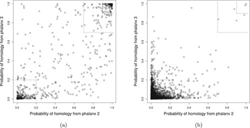
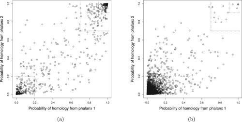
Figure 4 explores EPX-APR by comparing the CV probabilities of homology from phalanxes 2 and 3 for homologous versus non-homologous proteins. (The CV probabilities have to be used as the true homology status is unknown for the test data, and these two phalanxes illustrate well diversity in predictions.) For the homologous proteins in Figure 4(a), larger probabilities will lead to better ranking. The smaller and larger top-right corners in Figure 4(a) contain $55.1\mathrm{\%}$ and $58.8\mathrm{\%}$, respectively, of all the homologous proteins in the training data. These true homologues will be ranked high overall, as there are very few proteins in the same high-probability regions for non-homologues in Figure 4(b). It is also seen that some homologous proteins receive small probabilities. The bottom-left corner of Figure 4(a) contains $24.4\mathrm{\%}$ of all the homologous proteins in the training data. The same cell in Figure 4(b) has far more proteins – homologous proteins account for only $0.22\mathrm{\%}$ of cases where both probabilities are less than 0.2 – but there is clearly potential for poor ranking of some homologues. Diversity of the probabilities from the two LR models helps for other homologues, however. Figure 4(a) contains homologous proteins in the top-left and bottom-right, i.e., one of the two LRs assigns a high probability of homology, and ensembling over the two LR models will pull these homologues ahead in the ranking despite the poorer ranking from one of the models.

Figure 4. Training data 10-fold CV LR probability of homology from phalanx 2 versus phalanx 3 for phalanx formation algorithm optimizing APR: (a) homologous and (b) non-homologous proteins in the training data. In the smaller and larger top-right corners, the probabilities of homology from both phalanxes are greater than 0.90 and 0.70, respectively; whereas in the bottom-left corner, the probabilities are less than 0.20.

Further diversity is present for phalanx 1 versus phalanx 2 and phalanx 1 versus phalanx 3. Hence the APR score of 0.809 in Table 3 for the EPX-APR ensemble improves on the performances of the three individual phalanxes.

Similarly, Figure 5 compares the CV probabilities of homology for the two phalanxes constructed by minimizing RKL. The smaller and larger top-right corners of Figure 5(a) contain $60.0\mathrm{\%}$ and $65.46\mathrm{\%}$, respectively, of all the homologous proteins in the training data, better performance than seen in Figure 4(a) for APR. Proteins in these regions will be ranked high, as the same regions in Figure 5(b) for non-homologous proteins are sparse. The lower-left corner of Figure 5(a) contains $20.2\mathrm{\%}$ of the homologous proteins, but this is only $0.18\mathrm{\%}$ of all proteins in this subregion across both Figure 5(a) and Figure 5(b), slightly fewer than seen in Figure 4, and hence EPX-RKL assigns large probabilities for difficult-to-rank homologous proteins. Looking at the top-left and bottom-right corner of Figure 5(a) for homologous proteins we see more diversity between the two estimated probabilities than in Figure 5(b). Some of these harder to identify homologous proteins are therefore pulled up in the ranking by the more favourable probability, which explains the superior performance of EPX-RKL in Table 4 relative to models from either constituent phalanx.

Figure 5. Training data 10-fold CV LR probability of homology from phalanx 1 versus phalanx 2 for phalanx formation minimizing RKL: (a) homologous and (b) non-homologous proteins proteins in the training data. In the smaller and larger top-right corners, the probabilities of homology from both phalanxes are greater than 0.90 and 0.70, respectively; whereas in the bottom-left corner, the probabilities are less than 0.20.

Turning to diversity between the EPX-APR and EPX-RKL models, and to discover further knowledge for building models for data mining, Table 7 compares their respective ranking performances over the training-data homologous proteins, in four categories. The categories are constructed based on the CV ranks from the aggregated ensemble EPX-EOM. To create categories of homologous proteins across blocks with differing sizes, the EPX-EOM ranks are normalized to the range $[0,1]$ within each block by dividing each rank by the number of candidates in the block. These scores then divide the homologous proteins into four roughly equally size groups: those with the smallest normalized ranks, in the range $[0.00000,0.00264)$, are deemed ‘very easy’ to rank, and so on up to $[0.02051,0.50000)$ for ‘very hard '. For the ‘very easy’ and ‘easy’ categories, the ranks of EPX-APR are smaller (better) than those of EPX-RKL more often than they are larger. For the ‘hard’ and ‘very hard’ categories, the comparison is reversed: EPX-RKL's ranks are more often smaller. Kaushik et al. (2016) [64] point out that homologues that are evolutionary remote from their native proteins are more difficult to predict than evolutionary close homologues. The suggestion here is that EPX-APR performs better for easier to mine near homologues, whereas EPX-RKL performs better for harder to mine distant/remote homologues. In this perspective, diversity between the two data mining methods leads to them choosing diverse homologues.

Table 7. Comparison of ranking performance of EPX-APR versus EPX-RKL for all training-data homologous compounds, categorized by the overall ranking performance of EPX-EOM.

EPX-EOM		Homologous	Smaller rank from
normalized rank	Difficulty	proteins	APR	Tie	RKL
$[0.00000,0.00264)$	Very easy	323	59	223	41
$[0.00264,0.00868)$	Easy	325	117	103	105
$[0.00868,0.02051)$	Hard	323	118	63	142
$[0.02051,0.50000)$	Very hard	325	103	34	188
$[0.00000,0.50000)$	Overall	1296	397	423	476

Note: The best classifier in each category is highlighted using boldface.

To further verify our observation, we next investigate four example blocks of proteins chosen to illustrate how EPX-APR and EPX-RKL are diverse and complementary. Table 8 gives the APR, TOP1 and RKL metrics from CV for training blocks of proteins 95, 216, 96 and 238. In each block and for each assessment metric the top performer between EPX-APR and EPX-RKL is marked by boldface. Blocks 95 and 216 are fairly easy to rank as both EPX-APR and EPX-RKL assign relatively small ranks to all their respective homologues, i.e. the homologues are near to their respective native proteins. Nonetheless, EPX-APR does better, placing the single homologue in Block 95 at the very beginning of the list and placing the three homologues in Block 216 in positions 1, 2, and 4. APR is sensitive to small changes in ranks of homologous proteins at the head of a list. EPX-RKL performs slightly worse but has no impact on the aggregated performance: EPX-EOM's metrics are exactly the same as EPX-APR's. Block 96 is apparently much harder to rank. EPX-APR and EPX-RKL both place a homologue in the fourth position, but the second – a remote homologue – is far down the list at position 492 or 394, respectively. It is seen, however, that EPX-RKL performs better for both APR and RKL and that its superior performance is almost matched by EPX-EOM. Block 238 is also difficult in the sense that there are 50 homologues to rank, and the last homologue is always well down the list. Again, EPX-RKL performs better, even for the APR metric, and EPX-EOM's metrics are closer to those of EPX-RKL. It appears that EPX-APR performs better for blocks with close homologous proteins that are easy to rank, whereas EPX-RKL performs better for remote/distant homologues that are difficult to rank. In a nutshell, we discovered the following novel knowledge: Ensembling models from the two objectives automatically achieves near-optimal ranking performance relative to the best of the two models, a strategy that is practical for test data where the best model is not identified.

Table 8. Assessment metrics APR, TOP1 and RKL for EPX-APR, EPX-RKL and EPX-EOM from CV for training blocks 95, 216, 96 and 238.

	Proteins			Assessment metrics
Block	Total	Homologous	Mining method	APR	TOP1	RKL
95	1120	1	EPX-APR	1.0000	1	1
			EPX-RKL	0.0909	0	11
			EPX-EOM	1.0000	1	1
216	1068	3	EPX-APR	0.9167	1	4
			EPX-RKL	0.8333	1	6
			EPX-EOM	0.9167	1	4
96	974	2	EPX-APR	0.1270	0	492
			EPX-RKL	0.1275	0	394
			EPX-EOM	0.1274	0	415
238	861	50	EPX-APR	0.5651	1	584
			EPX-RKL	0.7811	1	249
			EPX-EOM	0.7125	1	346

Note: In each block, the top performance among EPX-APR and EPX-RKL is marked using boldface.

5.5. Computational gain of EPX-LR over EPX-RF

The time complexity of the ensemble of phalanxes is $\mathcal{O}(d^2)$, where d is the number of initial feature variables, and Table 9 shows the computation times (both training and testing) for EPX-LR, EPX-RF and RF on the protein homology data. The table also shows the number of processors used and amount of memory allocated for parallel computation of the three ensembles running on WestGrid⁴ (Western Canada Research Grid). For each of the 32 processors, 8 GB of memory was allocated. The computation times to train and test EPX-RF and EPX-LR were 1569 and 70–80 minutes, respectively. (EPX-LR is run with several metrics, hence the range of times.) The time for EPX-LR based on logistic regression is much smaller than for EPX-RF with RF as the base classifier. Through parallel computation, the computing time of EPX-LR was brought down to be similar to a single RF, for which training and test using one processor and 8 GB memory took 67 minutes. One can also easily assign more processors to further reduce the computation time of EPX.

Table 9. Parallel computation time in minutes for EPX-LR, EPX-RF and RF using Western Canada Research Grid (WestGrid).

Classifiers	Number of processors	Memory allocation (GB)	Elapsed time (Minute)
RF	1	8	67
EPX-RF	32	8	1569
EPX-LR	32	8	70–80

6. Discussion and conclusion

In machine learning and data science, an ensemble is considered as an aggregated collection of models. To build a powerful ensemble, the constituent base learners need to be strong and diverse. In this article, the world ‘strong’ stands for strong predictive ranking by a base learner. The proposed algorithm of phalanx formation groups a set of feature variables into diverse phalanxes guided by a ranking objective. Two phalanxes and their models are diverse in a sense that they predict well different sets of rare class objects (homologous proteins here). The algorithm keeps grouping feature variables into phalanxes until a set of feature variables help each other in a model, and ends up with more than one phalanx. In summary, EPX seeks to place good feature variables together in a phalanx to increase its strength, while exploiting different phalanxes to induce diversity between constituent base learners.

An excellent property of EPX is filtering weak/noise feature variables. A feature variable is considered weak if it shows poor predictive ranking performance: (i) individually in a model, (ii) jointly when paired with another feature variable in a model, and (iii) jointly when ensembled with another feature variable in different models. The algorithm also filters harmful phalanxes of feature variables. Harmful stands for weakening the predictive ranking performance of an ensemble comparing to the top predictive performances of individual base learners (i.e. phalanxes). A candidate phalanx is filtered out if it appears harmful with any other phalanx(es) used in the final ensemble. Therefore, the merging step of the algorithm of phalanx formation is sandwiched by filtering weak feature variables and candidate phalanxes.

A previously less highlighted property of the EPX algorithm is model selection. Regular model selection methods – such as forward stepwise selection, backward elimination, ridge regression [82], and the lasso [83] – select one subset of feature variables (which can be considered as a phalanx) and build one model. In contrast, EPX selects a collection of models (via subsets of features) and aggregates them in ensembles. Each of these models can be considered as an alternative to the models conveniently selected by other methods mentioned above. Furthermore, the constituent models in EPX rank diverse collections of rare class objects (homologous proteins here), which is similar to examining a problem from different vantage points.

Previous applications of EPX have used RF as the underlying base learner. Here, in this article, LR appears as a better base learner. The results of EPX using LR are reasonably close to the winners of the KDD Cup competition. These findings are encouraging and suggest considering other suitable base learners such as recursive partitioning [84], neural networks [85], etc., as best for a given application.

EPX is independently optimized for different evaluation metrics average precision and rank last here. This exemplifies the flexibility of EPX. The underlying base learner need not be rewritten, rather a specific metric is applied to guide phalanx formation. The choice of assessment metrics can be application dependent, with the goal of finding an ensemble of metrics with good overall performance. As observed, EPX-EOM can provide uniformly better performance even against models tuned specifically for one ranking criterion. APR is useful to mine near homologues, while RKL is helpful to mine remote homologues. The diversity in the assessment metrics APR and RKL injected further diversity in the models EPX-APR and EPX-RKL. The resulting diversity in the models EPX-APR and EPX-RKL enabled us to produce a better predictive model EPX-EOM via ensembling.

A hit curve can be obtained by plotting the number (or proportion) of hits of rare class objects against the number (or proportion) of shortlisted objects. A hit curve is a good measure of performance evaluation of a classifier when the objective is the ranking of the rare class objects [23]. Wang (2005) [47] showed that a hit curve is a better method of evaluating a highly unbalanced classification problem than misclssification error which is suitable for a balanced classification problem. In biomedical applications, a receiver operator characteristic (ROC) curve is constructed by plotting true positive rate (proportion of objects that were correctly predicted to be positive out of all positive objects) against the false positive rate (proportion of objects that are incorrectly predicted to be positive out of all negative objects). The true positive rate is also known as sensitivity and recall; and the false positive rate can be expressed as one minus specificity (proportion of objects that are correctly predicted to be negative out of all negative objects) [86,87]. On the other hand, a precision recall curve is obtained by plotting precision (proportion of true positives among those that are predicted positive) against recall [88,89]. Su et al. (2015) [90] established the relationships between a hit curve and a ROC curve and showed that average precision (APR) is approximately area under the ROC curve (AUC) times initial precision. Moreover, Fan and Zhu (2011) [91] showed that APR is a composite mean of precision and recall. As our application of this article is in ranking rare class objects which lean towards information retrieval, we used hit curve, APR and other associated assessment metrics rather than ROC, precision & recall curves and their AUCs.

As mentioned before, the choice of assessment metrics to ensemble is application dependent. The user should need to know the properties of the assessment metrics to find out a subset of diverse metrics. After that, a training dastset with an appropriate cross-validation procedure may be used to select the final set of assessment metrics to ensemble. For example, in biomedical applications, one may wish to consider the assessment metrics such as sensitivity, specificity, precision, recall, accuracy, F-measure, AUC, etc. as an ad-hoc set of diverse assessment metrics. Finally, the user may wish to use a training dataset with appropriate cross-validation to select a final set of assessment metrics to ensemble.

Future work may include extending EPX-EOM to linear regression and multi-class classification problems using variants of metrics such as mean squared error and misclassification rate, etc. It would also be interesting to examine if improvements can be achieved by aggregating ensembles of phalanxes based on different base learners as well.

The proposed methodology can also be applied to any data mining application with high-dimensional feature space where, metaphorically, the objective is to find a needle in a haystack. Firstly, the high-dimensional feature space will help building a strong predictive ensemble of phalanxes via splitting the set of features into smaller subsets. Secondly, both the easy and difficult to mine instances can be detected by ensembling across diverse assessment metrics, such as APR and RKL. For example, the proposed methodology may be useful in mining fraudulent credit card transactions [7], searching information on the world wide web [19], mining active biomolecules in drug-discovery [22], intrusion detection in internet surveillance [12], forecasting/prediction of air pollution/quality or exposure in air pollution epidemiology [92], and beyond.

Acknowledgements

We thank Professor Ron Elber, University of Texas at Austin, Texas, USA, for his help to understand the feature variables of this protein homology data. The Western Canada Research Grid (WestGrid) computational facilities of Compute Canada are gratefully acknowledged.

Disclosure statement

No potential conflict of interest was reported by the author(s).

Additional information

Funding

We acknowledge support from the Natural Sciences and Engineering Research Council of Canada (NSERC grants RGPIN-2021-03970, RGPIN-2014-04962 and RGPIN-2014-05227).

Notes

1 http://osmot.cs.cornell.edu/kddcup/datasets.html: Accessed 14 March 2022.

2 http://osmot.cs.cornell.edu/kddcup/protein_description.pdf: Accessed 14 March 2022.

3 http://osmot.cs.cornell.edu/cgi-bin/kddcup/newtable.pl?prob=bio: Accessed 14 March 2022.

4 http://www.westgrid.ca/: Accessed 14 March 2022.

Appendix

References

- Dokas P, Ertoz L, Kumar V, et al. Data mining for network intrusion detection. In: Proceedings NSF Workshop on Next Generation Data Mining; 2002. p. 21–30.
- Weiss GM. Mining with rare cases. In: Data mining and knowledge discovery handbook. Boston (MA): Springer; 2009. p. 747–757.
- Wu J, Xiong H, Chen J. COG: local decomposition for rare class analysis. Data Min Knowl Discov. 2010;20(2):191–220.
- Dongre SS, Malik LG. Rare class problem in data mining. Int J Adv Res Comput Sci. 2017;8(7):1102–1105.
- Zhou D, Karthikeyan A, Wang K, et al. Discovering rare categories from graph streams. Data Min Knowl Discov. 2017;31(2):400–423.
- Bolton RJ, Hand DJ. Statistical fraud detection: a review. Stat Sci. 2002;17(3):235–255.
- Bhusari V, Patil S. Application of hidden Markov model in credit card fraud detection. Int J Distrib Parallel Syst. 2011;2(6):203–211.
- Lippmann RP, Cunningham RK. Improving intrusion detection performance using keyword selection and neural network. Comput Netw. 2000 Oct;34(4):597–603.
- Sherif JS, Dearmond TG. Intrusion detection: systems and models. In: Proceedings Eleventh IEEE International Workshops on Enabling Technologies: Infrastructure for Collaborative Enterprises; 2002 Jun; Pittsburgh, PA. IEEE. p. 115–133.
- Kemmerer RA, Vigna G. Hi-DRA: intrusion detection for internet security. Proc IEEE. 2005 Oct;93(10):1848–1857.
- Maiti A, Sivanesan S. Cloud controlled intrusion detection and burglary prevention stratagems in home automation systems. In: 2012 2nd Baltic Congress on Future Internet Communications; 2012 Apr; Vilnius, Lithuania. IEEE. p. 182–186.
- Gendreau AA, Moorman M. Survey of intrusion detection systems towards an end to end secure internet of things. In: 2016 IEEE 4th International Conference on Future Internet of Things and Cloud (FiCloud); 2016 Aug. p. 84–90.
- Fienberg SE, Shmueli G. Statistical issues and challenges associated with rapid detection of bio-terrorist attacks. Stat Med. 2005 Feb;24(4):513–529.
- Peeters J. Method and apparatus for wide area surveillance of a terrorist or personal threat. US Patent 7, 109, 859; 2006. Available from: https://www.google.com/patents/US7109859
- Cohen K, Johansson F, Kaati L, et al. Detecting linguistic markers for radical violence in social media. Terror Political Violence. 2014;26(1):246–256.
- Gordon M, Pathak P. Finding information on the world wide web: the retrieval effectiveness of search engines. Inf Process Manag Int J. 1999 Mar;35(2):141–180.
- Nachmias R, Gilad A. Needle in a hyperstack. J Res Technol Educ. 2002;34(4):475–486.
- Al-Masri E, Mahmoud QH. Investigating web services on the world wide web. In: Proceedings of the 17th International Conference on World Wide Web, WWW '08; New York (NY), USA. ACM; 2008. p. 795–804.
- Baeza-Yates RA, Ribeiro-Neto BA. Modern information retrieval – the concepts and technology behind search. 2nd ed. Harlow: Pearson Education; 2011.
- Bleicher KH, Böhm HJ, Müller K, et al. A guide to drug discovery: hit and lead generation: beyond high-throughput screening. Nat Rev Drug Discov. 2003;2:369–378.
- Wang J, Hou T. Drug and drug candidate building block analysis. J Chem Inf Model. 2010;50(1):55–67. PMID: 20020714.
- Tomal JH, Welch WJ, Zamar RH. Exploiting multiple descriptor sets in QSAR studies. J Chem Inf Model. 2016;56(3):501–509.
- Zhu M, Su W, Chipman HA. LAGO: a computationally efficient approach for statistical detection. Technometrics. 2006;48(2):193–205. Available from: http://www.jstor.org/stable/25471156
- Chawla NV. Data mining for imbalanced datasets: an overview. Boston (MA): Springer US; 2010. Chapter 40; p. 875–886.
- Tayal A, Coleman TF, Li Y. RankRC: large-scale nonlinear rare class ranking. IEEE Trans Knowl Data Eng. 2015;27(12):3347–3359.
- Hsu GG, Tomal JH, Welch WJ. EPX: an R package for the ensemble of subsets of variables for highly unbalanced binary classification. Comput Biol Med. 2021;136:104760.
- Kearsley SK, Sallamack S, Fluder EM, et al. Chemical similarity using physiochemical property descriptors. J Chem Inf Comput Sci. 1996;36(1):118–127.
- Kishida K. Property of average precision and its generalization: an examination of evaluation indicator for information retrieval experiments. Tokyo: Japan National Institute of Informatics; 2005.
- Fu Y, Pan R, Yang Q, et al. Query-adaptive ranking with support vector machines for protein homology prediction. In: Chen J, Wang J, Zelikovsky A, editors. Bioinformatics research and applications. Berlin: Springer; 2011. p. 320–331.
- Tomal JH, Welch WJ, Zamar RH. Ensembling classification models based on phalanxes of variables with applications in drug discovery. Ann Appl Stat. 2015;9(1):69–93.
- Karplus K, Barrett C, Hughey R. Hidden Markov models for detecting remote protein homologies. Bioinformatics. 1998;14(10):846–856.
- Hochreiter S, Heusel M, Obermayer K. Fast model-based protein homology detection without alignment. Bioinformatics. 2007;23(14):1728–1736.
- Ma J, Wang S, Wang Z, et al. MRFalign: protein homology detection through alignment of Markov random fields. PLoS Comput Biol. 2014 Mar;10(3):1–12.
- Yen SJ, Lee YS. Under-sampling approaches for improving prediction of the minority class in an imbalanced dataset. Berlin: Springer; 2006. p. 731–740.
- Liu R, Hall LO, Bowyer KW, et al. Synthetic minority image over-sampling technique: How to improve AUC for glioblastoma patient survival prediction. In: 2017 IEEE International Conference on Systems, Man, and Cybernetics (SMC); 2017. p. 1357–1362.
- Breiman L. Bagging predictors. Mach Learn. 1996;24(2):123–140.
- Dietterich TG. An experimental comparison of three methods for constructing ensembles of decision trees: bagging, boosting, and randomization. Mach Learn. 2000;40(2):139–157.
- Breiman L. Random forests. Mach Learn. 2001 Oct;45(1):5–32.
- Friedman JH. Stochastic gradient boosting. Comput Stat Data Anal. 2002;38(4):367–378.
- Cannings TI, Samworth RJ. Random-projection ensemble classification. J R Stat Soc Series B Stat Methodol. 2017;79(4):959–1035.
- Chawla NV, Lazarevic A, Hall LO, et al. SMOTEBoost: improving prediction of the minority class in boosting. In: Lavrač N, Gamberger D, Todorovski L, et al., editors. Knowledge discovery in databases: PKDD 2003; Berlin: Springer; 2003. p. 107–119.
- Chen C, Breiman L. Using random forest to learn imbalanced data. Berkeley: University of California; 2004 Jan.
- Lin HI, Nguyen MC. Boosting minority class prediction on imbalanced point cloud data. Appl Sci. 2020;10(3):Article no. 973.
- Melville P, Mooney RJ. Constructing diverse classifier ensembles using artificial training examples. In: Proceedings of the IJCAI-2003; 2003 Aug; Acapulco, Mexico. p. 505–510.
- Kuncheva LI, Whitaker CJ. Measures of diversity in classifier ensembles and their relationship with the ensemble accuracy. Mach Learn. 2003;51(2):181–207.
- Brown G, Wyatt JL, Tino P, et al. Managing diversity in regression ensembles. J Mach Learn Res. 2005;6(9):1621–1650.
- Wang Y. Statistical methods for high throughput screening drug discovery data [dissertation]. Waterloo: University of Waterloo; 2005.
- Gupta R, Audhkhasi K, Narayanan S. Training ensemble of diverse classifiers on feature subsets. In: 2014 IEEE International Conferences on Acoustic, Speech and Signal Processing (ICASSP); 2014. p. 2951–2955.
- Tomal JH, Welch WJ, Zamar RH. Discussion of random-projection ensemble classification by T. I. Cannings and R. J. Samworth.. J R Stat Soc B Stat Methodol. 2017;79(4):1024–1025.
- Ho TK. The random subspace method for constructing decision forests. IEEE Trans Pattern Anal Mach Intell. 1998;20(8):832–844.
- Koonin EV, Galperin MY. Sequence – Evolution – Function: computational approaches in comparative genomics. Boston (MA): Kluwer Academic; 2003.
- Bordoli L, Kiefer F, Arnold K, et al. Protein structure homology modelling using SWISS-MODEL workspace. Nat Protoc. 2009 Feb;4:1–13.
- Söding J. Protein homology detection by HMM-HMM comparison. Bioinformatics. 2005;21(7):951–960.
- Nam SZ, Lupas AN, Alva V, et al. The MPI bioinformatics toolkit as an integrative platform for advanced protein sequence and structure analysis. Nucleic Acids Res. 2016 Apr;44(W1):W410–W415.
- Bork P, Koonin EV. Predicting functions from protein sequences – where are the bottlenecks? Nat Genet. 1998 Apr;18(4):313–318.
- Henn-Sax M, Höcker B, Wilmanns M, et al. Divergent evolution of (βα)8-barrel enzymes. Biol Chem. 2001 Sep;382:1315–1320.
- Kinch LN, Wrabl JO, Sri Krishna S, et al. CASP5 assessment of fold recognition target predictions. Proteins: Struct Funct Genet. 2003 Oct;53:395–409.
- Marks DS, Colwell LJ, Sheridan R, et al. Protein 3D structure computed from evolutionary sequence variation. PLoS One. 2011 Dec;6(12):1–20.
- Meier A, Söding J. Automatic prediction of protein 3D structures by probabilistic multi-template homology modeling. PLoS Comput Biol. 2015 Oct;11(10):1–20.
- Sinha S, Eisenhaber B, Lynn AM. Predicting protein function using homology-based methods. Singapore: Springer; 2018. p. 289–305.
- Waterhouse A, Rempfer C, Heer FT, et al. SWISS-MODEL: homology modelling of protein structures and complexes. Nucleic Acids Res. 2018 May;46(W1):W296–W303.
- Eddy SR. Profile hidden Markov models. Bioinformatics. 1998;14(3):755–763.
- Eddy SR. Accelerated profile HMM searches. PLoS Comput Biol. 2011 Oct;7(10):1–16.
- Kaushik S, Nair AG, Mutt E, et al. Rapid and enhanced remote homology detection by cascading hidden Markov model searches in sequence space. Bioinformatics. 2016 Feb;32(3):338–344.
- Zhang C, Zheng W, Mortuza SM, et al. DeepMSA: constructing deep multiple sequence alignment to improve contact prediction and fold-recognition for distant-homology proteins. Bioinformatics. 2019 Nov;36(7):2105–2112.
- Zhu M. Recall, precision and average precision. Waterloo: Department of Statistics and Actuarial Science, University of Waterloo; 2004.
- Zamar RH, Welch WJ, Yan G, et al. Partial results for KDD cup 2004; 2004. Available from: http://stat.ubc.ca/will/ddd/kdd_result.html
- Vallat BK, Pillardy J, Májek P, et al. Building and assessing atomic models of proteins from structural templates: learning and benchmarks. Proteins. 2009 Sep;76(4):930–945.
- Teodorescu O, Galor T, Pillardy J, et al. Enriching the sequence substitution matrix by structural information. Proteins: Struct Funct Genet. 2004;54(1):41–48.
- Vallat BK, Pillardy J, Elber R. A template-finding algorithm and a comprehensive benchmark for homology modeling of proteins. Proteins. 2008 Aug;72(3):910–928.
- Haddad Y, Adam V, Heger Z. Ten quick tips for homology modeling of high-resolution protein 3D structures. PLoS Comput Biol. 2020 Apr;16(4):1–19.
- Vyas V, Ukawala R, Ghate M, et al. Homology modeling a fast tool for drug discovery: current perspectives. Indian J Pharm Sci. 2012 Mar;74:1–17.
- Makigaki S, Ishida T. Sequence alignment using machine learning for accurate template-based protein structure prediction. Bioinformatics. 2020 Jun;36(1):104–111.
- Senior A, Evans R, Jumper J, et al. Improved protein structure prediction using potentials from deep learning. Nature. 2020 Jan;577:706–710.
- Bachem O, Lucic M, Krause A. Coresets for nonparametric estimation – the case of DP-means. In: Bach F, Blei D, editors. Proceedings of the 32nd International Conference on Machine Learning; Jul 7–9; Lille, France. PMLR; 2015. p. 209–217. (Proceedings of Machine Learning Research; Vol. 37).
- Bachem O, Lucic M, Krause A. Scalable k-means clustering via lightweight coresets. In: Proceedings of the 24th ACM SIGKDD International Conference on Knowledge Discovery & Data Mining, KDD '18; London, UK. ACM SIGKDD; 2018. p. 1119–1127.
- Hirschberger F, Forster D, Lücke J. Large scale clustering with variational EM for Gaussian mixture models. arXiv:181000803; 2019.
- Tsai CF, Lin WC, Ke SW. Big data mining with parallel computing: a comparison of distributed and mapreduce methodologies. J Syst Softw. 2016;122:83–92.
- Pfahringer B. The Weka solution to the 2004 KDD cup. ACM SIGKDD Explorations Newsletter. 2004;6(2):117–119.
- Freund Y, Schapire RE. A decision-theoretic generalization of on-line learning and an application to boosting. J Comput Syst Sci. 1997;55(1):119–139.
- Cortes C, Vapnik V. Support-vector networks. Mach Learn. 1995;20(3):273–297.
- Hastie T, Tibshirani R, Friedman J. The elements of statistical learning: data mining, inference, and prediction. 2nd ed. New York: Springer; 2009.
- Tibshirani R. Regression shrinkage and selection via the lasso. J R Stat Soc B Stat Methodol. 1996;58(1):267–288.
- Breiman L, Friedman J, Stone C, et al. Classification and regression trees. New York: Chapman and Hall/CRC; 1984.
- Ripley BD. Pattern recognition and neural networks. Cambridge (UK): Cambridge University Press; 1996.
- Campbell G, Ratnaparkhi MV. An application of Lomax distributions in receiver operating characteristic (ROC) curve analysis. Commun Stat Theory Methods. 1993;22(6):1681–1687.
- Pepe MS. Receiver operating characteristic methodology. J Am Stat Assoc. 2000;95(449):308–311.
- Boyd K, Eng KH, Page CD. Area under the precision-recall curve: point estimates and confidence intervals. In: Joint European conference on machine learning and knowledge discovery in databases. Prague (Czech Republic): Springer; 2013. p. 451–466.
- Sofaer HR, Hoeting JA, Jarnevich CS. The area under the precision-recall curve as a performance metric for rare binary events. Methods Ecol Evol. 2019;10(4):565–577.
- Su W, Yuan Y, Zhu M. A relationship between the average precision and the area under the ROC curve. In: Proceedings of the 2015 International Conference on The Theory of Information Retrieval. Northampton (MA): ACM; 2015. p. 349–352.
- Fan G, Zhu M. Detection of rare items with target. Stat Interface. 2011;4(1):11–17.
- Bellinger C, Jabbar MSM, Zaïane O, et al. A systematic review of data mining and machine learning for air pollution epidemiology. BMC Public Health. 2017;17(907):1–19.