Stability of principal components under normal and non-normal parent populations and different covariance structures scenarios

Abstract

Principal Component Analysis (PCA) is one of the most used multivariate techniques for dimension reduction assuming nowadays a particular relevance due to the increasingly common large datasets. Being mainly used as a descriptive/exploratory tool it does not require any explicit a priori assumption. However, regardless the parent population miss/unknown characterization, sample principal components are often used to characterize the parent population structure, as these are frequently targeted to visualize multivariate datasets on a 2D graphical display or to infer the first two latent dimensions. In this context, although the main goal might not be inferential, sample principal components may fail to provide a valid solution as principal components may vary considerably, depending on the extracted sample. The stability of the PCA solution is here studied considering normal and non-normal parent populations and three covariance structures scenarios. In addition, the effects of the covariance parameter, the dimension and the size of the sample are also investigated via Monte Carlo simulations. This study aims to understand how stability varies with the population and sample features, characterize the conditions under which PCA results are expected to be stable, and study a sample criterion for PCA stability.

Keywords:

• Principal components
• eigenvectors
• nonnormality
• simulation
• stability

1. Introduction

Principal Components Analysis (PCA) is still nowadays one of the most commonly used multivariate statistical analysis technique [1,2]. Over the years, it has been applied in many different scientific fields (see, e.g. [3]) being mainly used as a dimension reduction tool. Despite this main use, PCA has, as frequently, been employed as a method to visualize multivariate datasets on a low-dimensional graphical display [4] by typically converting the original data into two-dimensional data, restricting, in this case, the analysis to a two dimension reduction problem (first two principal components) [5]. Further, PCA is often used to define uncorrelated latent variables (components) at the expense of observed ones. Important areas of application with considerable interest include (i) allometry studies [6,7], to partition morphometric variation into components that separately describe the size and shape of living organisms (e.g. [8–10]), (ii) drug design and discovery, aiming to relate the structure of chemicals to their physical properties in the context of quantitative structure–activity relationships (QSAR) studies (e.g. [11]), and (iii) multivariate time series studies including, e.g. meteorological [1,12,13], prices or crime rate quantities, where observations, typically made at different time points, are non-independent. Being outside of the scope of this study, non-independence between observations is here not addressed. However, as this study is restricted to the use of PCA for descriptive (not inferential) purposes, non-independence is not expected to affect this goal [3].

In all the above real applications, although PCA is almost exclusively used as an exploratory tool, sample principal components structure is used to characterize the corresponding population principal components structure, typically retaining only the first couple of axes [14,15] being the remaining typically less informative and more difficult to interpret [1]. Hence, in these applications it is of critical importance that sample principal components span over a narrow vicinity of their population counterparts, to reflect the true underlying structure.

In general, the concept of stability of an analysis method is defined by the degree of sensitivity of the analysis to the variations in the input conditions [16]. Furthermore, the stability concept may be interpreted as related to the degree of variation of the solution depending on the considered sample (sample pattern) and its legitimacy to be interpreted as representing the population structure (true pattern) (e.g. [17]). Hence, PCA stability or repeatability is related to the change imposed on the linear coefficients that define PC driven by sampling variability. Taking stability as a prerequisite to useful interpretation [18], then it is advisable to know which conditions may hinder PCA stability.

PCA stability is commonly researched as depending on the data distributional assumption (e.g. [18]), the underlying covariance matrix (e.g. [19]) and/or features as the number of variables (p) and the sample size (e.g. [20]).

Normality assumption is not mandatory to perform a PCA [3]. However, the lack of normality may affect PCA results in multiple ways. In particular, the optimal (exact or asymptotic) properties of the Maximum Likelihood Estimators (MLE) of the true covariance matrix $\mathbf{\Sigma }$ (and related eigen parameters) can not be assumed, potentially inducing estimated PC substantiality biased. Also, without the normality assumption PC cannot be assumed to define the principal axes of the family of p-dimensional ellipsoid and represent contours of constant probability for the distribution of the random vector $\mathbf{x}$. It is generally assumed that, given enough structure for the extraction of PC, the stability or repeatability of PCA results does not depend heavily on the normality on the data [21]. Further, Daudin et al. [17] studied four different real datasets presenting an increasing degree of instability, without any underlying assumption, and conclude that data structure by itself is not enough to define a general rule that could replace a stability analysis.

The variances of the population PC are given by the eigenvalues ${\lambda }_j(j=1,\dots ,p)$ of the population covariance matrix $\mathbf{\Sigma }$. When $\mathbf{A}\mathbf{\Sigma }{\mathbf{A}}^{\prime }={\sigma }^2\mathbf{I}$, (where $\mathbf{A}$ is the matrix whose columns are the elements of the eigenvectors ${\mathit{\alpha }}_j$ of the covariance matrix), the covariance structure has p equal eigenvalues and is termed spherical.

As such, several statistics related to the degree of distinctiveness of the eigenvalues (sphericity) have been used to decide whether or not is it worthwhile to perform a PCA [22]. For spherical covariance structures the arithmetic mean is equal to the geometric mean of the eigenvalues of $\mathbf{\Sigma }$, that is, the statistic (1) $\frac{\prod _{j=1}^p{\lambda }_j^{1/p}}{\sum _{j=1}^p{\lambda }_j/p}$(1) equals 1 [23,24].

In this context, the further statistical test of equality between the eigenvalues of the population covariance matrix (all or a particular subset) has no practical value, as it assumes a multivariate normal distribution which is often not satisfied [3].

The number of variables (p) and the size of the sample (n) are also expected to interfere with the stability of the PC. The consistency of MLE ensures that the sample covariance will approximate increasingly better the population covariance as n increases. However, the consistency of a principal component is driven not only by the sample size, but also by its relationship with the dimension p and the relative sizes of the several leading eigenvalues [4].

Given the above described potential effects over PCA results, this work aimed at studying the stability of the PCA solution under normal and non-normal parent populations and different covariance structures varying both the type of pattern and the magnitude of the parameters to reflect different types of data scenarios. The interaction between the effects of the data distribution, the covariance pattern, the sample size and the population dimension was also investigated. In summary, our goals included (i) understand how stability varies with population characteristics (dimension, data distribution, covariance matrix type and parameters) and sample size; (ii) characterize conditions under which PCA results are expectedly stable, and (iii) establish a sample criterion for PCA stability.

This manuscript is structured as follows. Section 2 defines the covariance structures considered in this study. Sections 3 and 4 describe, respectively, the metrics used to evaluate PCA stability and the simulation procedure. In Sections 5 and 6 we present the simulation results and two real applications in the context of allometry studies. Conclusions are presented in the last section describing the limitations and presenting guidelines about when to use the study findings.

2. Covariance structures

In this study we have considered the covariance structures known as compound symmetry and first-order autoregressive, which are among the most commonly assumed (e.g. [25,26]), and the more general toeplitz covariance matrix type, that encompass the former two. Next, we briefly describe these structures:

• Compound symmetry (CS): Structure defined by a covariance matrix with constant variances ${\sigma }^2$ and non-zero constant covariances ${\sigma }_{i,j}(i\ne j)$, such that ${\sigma }_{i,j}={\sigma }^2\rho (i\ne j)$ (two parameters), where ${\rho }_{i,j}=\rho$ represents the correlation between the ith and the jth variables. This type of patterned covariance structure is often observed in real data, namely, e.g. among certain biological variables such as the sizes of living things [27].

• First-order autoregressive (AR(1)): Structure defined by a covariance matrix with ${\sigma }^2$ on the main diagonal and ${\sigma }_{i,j}={\sigma }^2{\rho }^{|i-j|}(i\ne j)$ on the other diagonals, where $|i-j|$ is the distance from the main diagonal. Hence, characterized by constant variances and exponential decreasing covariances with increasing lag $|i-j|$ (two parameters). Note that the speed of convergence of the covariance ${\sigma }_{i,j}={\rho }^{|i-j|}$ towards zero as $i\to \mathrm{\infty }$, given a fixed position j, depends on the value of ρ, being higher for lower values of ρ.

• Toeplitz (TOEPLITZ): Structure defined by a covariance matrix characterized by constant variances and decreasing covariances ${\sigma }_{i,j}={\sigma }^2{\rho }_{|i-j|}(i\ne j)$ with lag $|i-j|$ (p parameters). The values of ${\rho }_1,\dots ,{\rho }_{|p-1|}$ were defined by building a sequence between ${\rho }_{|p-1|}=\rho$ and 1 with an increment of $(1-\rho )/(p-1)$.

These three types of covariance matrices, conjugated with the different space dimensions (p) and correlation values (ρ), encompass different levels of sphericity generically following the order TOEPLITZ < CS < AR(1).

3. Stability

In this section we describe the metrics used to evaluate stability (Sub-section 3.1) and define a sample criterion for stability diagnosis (Sub-section 3.2).

3.1. Stability metrics

PCA stability depends on how close the estimated principal components (sample) are to the true principal components (population). Mathematically, this closeness may be evaluated by the similarity between population and sample eigenvectors [20]. One natural way of measuring this closeness (or degree of overlap) uses the angular displacement between the vectors [28]. Let ${\mathit{\alpha }}_j$ and ${\mathbf{a}}_j$ represent the normalized eigenvectors of the covariance matrices $\mathbf{\Sigma }$ and $\mathbf{S}$, respectively. PC stability may be measured by the directional displacement between sample and population principal components, taking the inner product of the two vectors (2) $\cos ({\theta }_j)={\mathbf{a}}_j^{\prime }{\mathit{\alpha }}_j$(2) where ${\theta }_j,(j=1,\dots ,p)$ is the angle between ${\mathit{\alpha }}_j$ and ${\mathbf{a}}_j$. Perfect stability is therefore characterized by an absolute cosine equal to 1. In this study, the jth PC is defined as stable if the correspondent angular displacement ${\theta }_j$ is such that $0.95\le |cos({\theta }_j)|\le 1$ [21]. The empirical sampling distribution of ${\theta }_j$ was used to analyse the chance of having a stable solution.

The angle defined according to (2(2) $\cos ({\theta }_j)={\mathbf{a}}_j^{\prime }{\mathit{\alpha }}_j$(2) ) allows to evaluate the individual eigenvector displacement. To account for a sub-group of eigenvectors, it can be considered a cumulative measure of the angular displacement. In particular, the displacement between subspaces generated by the first k sample and population eigenvectors may be defined by (3) $G_k=\sum _{j\le k}({\mathbf{a}}_j^{\prime }{\mathit{\alpha }}_j{)}^2(k=1,\dots ,p)$(3) which measures the global stability of the first k axes [17]. The closer this measure is to k, the more stable is the space spanned by the first k principal components. Thus, it may be seen as an index of subspaces coincidence, ranging from 0 (all orthogonal subpaces) to k (all coincident subspaces). Perfect stability correspond to the value $G_k=k$, when all estimated subspaces coincide perfectly with true subspaces.

3.2. Sample criterion for stability diagnosis

Principal components are grouped into subspaces preserving the order determined by its variance. This subspaces my be spanned by a single eigenvector or, in the case of degeneracy (i.e. indistinguishability in terms of their variance), by multiple eigenvectors. In this case, estimated eigenvectors tend to mix the population counterparts arbitrarily and sample eigenvectors are, in fact, linear combinations of true eigenvectors [29].

Let ${\ell }_k$ and ${\lambda }_k$ represent, respectively, the eigenvalues of the covariance matrices $\mathbf{\Sigma }$ and $\mathbf{S}$. First-order approximations of eigenpairs are given by [30] (4) $\begin{array}{rl}{\ell }_k& \approx {\lambda }_k+{\lambda }_k(2/n{)}^{1/2}\end{array}$(4) (5) $\begin{array}{rl}{\mathbf{a}}_k& \approx {\mathit{\alpha }}_k+\frac{{\ell }_k-{\lambda }_k}{{\lambda }_k-{\lambda }_{k+1}}{\mathit{\alpha }}_{k+1},(k=1,\dots ,p-1).\end{array}$(5) Hence, (6) $\begin{array}{rl}{\mathbf{a}}_k-{\mathit{\alpha }}_k& \approx \frac{se({\lambda }_k)}{\mathrm{\Delta }{\lambda }_k}{\mathit{\alpha }}_{k+1}\end{array}$(6) (7) $\begin{array}{rl}\mathrm{with}\frac{se({\lambda }_k)}{\mathrm{\Delta }{\lambda }_k}& =\frac{{\lambda }_k(2/n{)}^{1/2}}{{\lambda }_k-{\lambda }_{k+1}}.\end{array}$(7) Equation (4(4) $\begin{array}{rl}{\ell }_k& \approx {\lambda }_k+{\lambda }_k(2/n{)}^{1/2}\end{array}$(4) ) shows that the sampling error in the eigenvalue (${\ell }_k-{\lambda }_k=se({\lambda }_k)$) is independent of its spacing to the nearest eigenvalue (${\lambda }_k-{\lambda }_{k+1}=\mathrm{\Delta }{\lambda }_k$). In contrast, from Equations (5(5) $\begin{array}{rl}{\mathbf{a}}_k& \approx {\mathit{\alpha }}_k+\frac{{\ell }_k-{\lambda }_k}{{\lambda }_k-{\lambda }_{k+1}}{\mathit{\alpha }}_{k+1},(k=1,\dots ,p-1).\end{array}$(5) ) to (7(7) $\begin{array}{rl}\mathrm{with}\frac{se({\lambda }_k)}{\mathrm{\Delta }{\lambda }_k}& =\frac{{\lambda }_k(2/n{)}^{1/2}}{{\lambda }_k-{\lambda }_{k+1}}.\end{array}$(7) ) it is clear that the sampling error in a particular eigenvector (${\mathbf{a}}_k-{\mathit{\alpha }}_k$) varies inversely with the spacing to the nearest eigenvalue ($\mathrm{\Delta }{\lambda }_k$). In particular, Equation (6(6) $\begin{array}{rl}{\mathbf{a}}_k-{\mathit{\alpha }}_k& \approx \frac{se({\lambda }_k)}{\mathrm{\Delta }{\lambda }_k}{\mathit{\alpha }}_{k+1}\end{array}$(6) ) shows that if the sampling error in the eigenvalue, $se({\lambda }_k)$, is of the same magnitude as the spacing, $\mathrm{\Delta }{\lambda }_k$, then the sampling error in the eigenvector will be comparable to the nearest eigenvector. This indistinguishability leads to unstable solutions in the sense that any combination of the eigenvectors in the subspace is also a possible eigenvector. Furthermore, different samples may lead to different linear combinations of the nearby eigenvectors resulting in extensively different patterns from one sample to another [30].

As sample eigenvalues are maximum likelihood estimates of correspondent true eigenvalues, to make practical use of Equation (7(7) $\begin{array}{rl}\mathrm{with}\frac{se({\lambda }_k)}{\mathrm{\Delta }{\lambda }_k}& =\frac{{\lambda }_k(2/n{)}^{1/2}}{{\lambda }_k-{\lambda }_{k+1}}.\end{array}$(7) ), true parameters may be replaced by the respective sample counterparts. By doing so it is possible to establish a sample criterion for eigenvectors stability. Hence, let (8) $\frac{se({\ell }_k)}{\mathrm{\Delta }{\ell }_k}=\frac{{\ell }_k(2/n{)}^{1/2}}{({\ell }_k-{\ell }_{k+1})}(k=1,\dots ,p-1)$(8) be the sample counterpart of the ratio defined in (7(7) $\begin{array}{rl}\mathrm{with}\frac{se({\lambda }_k)}{\mathrm{\Delta }{\lambda }_k}& =\frac{{\lambda }_k(2/n{)}^{1/2}}{{\lambda }_k-{\lambda }_{k+1}}.\end{array}$(7) ). Then,

• if $se({\ell }_k)/\mathrm{\Delta }{\ell }_k>1$, i.e. if the eigenvalue spacing ($\mathrm{\Delta }{\ell }_k$) is smaller than the sampling error in the eigenvalue $(se({\ell }_k))$, the noise-to-signal ratio is too high to disentangle the eigenvectors (in terms of their variance). Hence, these degenerated subspaces correspond to solutions as unstable as (8(8) $\frac{se({\ell }_k)}{\mathrm{\Delta }{\ell }_k}=\frac{{\ell }_k(2/n{)}^{1/2}}{({\ell }_k-{\ell }_{k+1})}(k=1,\dots ,p-1)$(8) ) is far-above 1;

• if $se({\ell }_k)/\mathrm{\Delta }{\ell }_k<1$, i.e. if the eigenvalue spacing ($\mathrm{\Delta }{\ell }_k$) exceeds the sampling error in the eigenvalue $(se({\ell }_k))$, the low noise-to-signal ratio ensures the disentanglement of the eigenvectors. Hence, these non-degenerated subspaces correspond to solutions as stable as (8(8) $\frac{se({\ell }_k)}{\mathrm{\Delta }{\ell }_k}=\frac{{\ell }_k(2/n{)}^{1/2}}{({\ell }_k-{\ell }_{k+1})}(k=1,\dots ,p-1)$(8) ) is far-under 1.

Let X represent the continuous statistic $se({\ell }_k)/\mathrm{\Delta }{\ell }_k$ and Y the binary random variable classifying the kth PC as stable¹ (Y = 0) or unstable (Y = 1), such that higher values of X provide stronger support for the occurrence of unstable PCA solutions (Y = 1). Consider $F_1(x)$ and $F_0(x)$ to represent the conditional distribution functions of X given Y = 1 and Y = 0, respectively, i.e. (9) $\begin{array}{rl}{F}_1(x)& =\mathrm{I}\mathrm{P}(\frac{{\ell }_k(2/n{)}^{1/2}}{{\ell }_k-{\ell }_{k+1}}\le x|Y=1)\end{array}$(9) (10) $\begin{array}{rl}{F}_0(x)& =\mathrm{I}\mathrm{P}(\frac{{\ell }_k(2/n{)}^{1/2}}{{\ell }_k-{\ell }_{k+1}}\le x|Y=0)\end{array}$(10) Hence, (11) $1-F_1(x)=\mathrm{I}\mathrm{P}(\frac{{\ell }_k(2/n{)}^{1/2}}{{\ell }_k-{\ell }_{k+1}}>x|Y=1)$(11) and $F_0(x)$ define, respectively, the Sensitivity ($Sens(x)$) and the Specificity ($Spec(x)$) of ratio $se({\lambda }_k)/\mathrm{\Delta }{\ell }_k$ as a statistic for stability diagnosis. Then, (12) $ROC(p)=1-F_1(F_0^{-1}(1-p)),(0\le p\le 1)$(12) where $F_0^{-1}(1-p)=inf\{x\in \mathrm{IR}:F_0(x)\ge 1-p\}$, defines the ROC (Receiver Operating Characteristic) curve which allows to (i) evaluate the discriminatory ability of the ratio $se({\lambda }_k)/\mathrm{\Delta }{\ell }_k$ to assign a PCA solution as stable/unstable, and (ii) find the optimal threshold that maximizes the correct classification of a PCA solution as stable or unstable.

This curve is a monotone increasing function mapping $Sens(x)$ vs. $1-Spec(x)$. An uninformative diagnosis tool is represented by the line with unit slope, $\mathrm{ROC}(p)=p$, i.e. $Sens(x)=1-Spec(x)$. The optimal threshold $x^{\ast }$ can be estimated maximizing overall correct classification, i.e. (13) $x^{\ast }=\underset{x}{\mathrm{argmax}}\{Sens(x)-(1-Spec(x))\}.$(13) The ROC curve is typically described using the Area Under Curve (AUC) index, defined by $\mathrm{AUC}={\int }_0^1\mathrm{ROC}(p)\mathrm{d}p$.

A perfect diagnosis tool has an $\mathrm{AUC}=1$ and a diagonal line, corresponding to an uninformative tool, has an $\mathrm{AUC}=0.5$. If two curves are order in the sense that ${\mathrm{ROC}}_A(p)\ge {\mathrm{ROC}}_B(p)$, then their $\mathrm{AUC}$ statistics are also ordered ${\mathrm{AUC}}_A\ge {\mathrm{AUC}}_B$, implying that the diagnosis tool works better for situation A than for situation B.

4. Simulation study

In this study we conducted a Monte Carlo (MC) simulation to analyse the stability of PCA as a function of the parent population (normal vs. non-normal), the number of variables (p), the type of covariance pattern and its parameters (ρ) and sample size (n).

The covariance matrix was defined by the correlation structure as only standardized variables were considered. Two different populations were simulated: (i) a multivariate normal population given a specific patterned covariance matrix, and (ii) a multivariate non-normal population with the same covariance matrix. Simulated multivariate normal data were generated using the function rmvnorm, from mvtnorm R package [31]. Given a specific mean vector and a covariance matrix, this algorithm transforms univariate to multivariate normal random values via a spectral decomposition [32]. Non-normal data were generated using the function mnonr, from mnonr R package [33]. In particular, multivariate nonnormal random numbers with the desired intercorrelations were generated following Vale and Maurelli [34] that extended Fleishman [35] method in which a nonnormal random variable is obtained from the linear combination of the first three powers of a standard normal variable (polynomial transformation). This transformation is used to obtain random samples from some nonnormal distributions with given skewness and kurtosis. Considering the asymptotic sampling distributions for univariate skweness and kurtosis [36], high order quantiles were used to approximately estimate absolute lower (skewness and kurtosis) bounds for nonnormality.

For each value of p, 5000 random samples with a specific sample size (see Table 1) were drawn, with replacement, from each population. For each sample, we estimated the true covariance/correlation matrix and, based on it, performed a PCA, obtaining the correspondent eigenvalues and eigenvectors. These sample eigenpairs were then used to calculate the measures described in Section 3. In summary, we provide an outline of the simulation process:

1. Generation of 5000 random samples, with replacement, from multivariate normal and non-normal populations, varying the type of covariance matrix and parameter ρ, the number of variables p and sample size n (Table 1);

2. Performance of a PCA, on the randomly sampled data, by spectral decomposition of the sample covariance matrix;

3. Evaluation of stability according to (2(2) $\cos ({\theta }_j)={\mathbf{a}}_j^{\prime }{\mathit{\alpha }}_j$(2) ) and (3(3) $G_k=\sum _{j\le k}({\mathbf{a}}_j^{\prime }{\mathit{\alpha }}_j{)}^2(k=1,\dots ,p)$(3) );

4. Evaluation of (8(8) $\frac{se({\ell }_k)}{\mathrm{\Delta }{\ell }_k}=\frac{{\ell }_k(2/n{)}^{1/2}}{({\ell }_k-{\ell }_{k+1})}(k=1,\dots ,p-1)$(8) );

5. Estimation of optimal thresholds by (13(13) $x^{\ast }=\underset{x}{\mathrm{argmax}}\{Sens(x)-(1-Spec(x))\}.$(13) ) as a function of the type of covariance matrix, the number of variables and parent population.

5. Results

5.1. Individual eigenvector angular displacement

Figure 1 shows the MC distribution of angular displacement (AD, in degrees) between the population and sample eigenvectors as a function of the type of covariance matrix, the parameter ρ, the number of variables (p) and sample size (n), for both normal and non-normal parent populations, regarding the first (Figure 1(a)) and second (Figure 1(b)) eigenvectors.

Figure 1. Estimated densities of angular displacement (degrees) between the population and sample eigenvectors as a function of covariance matrix pattern, covariance matrix parameter (ρ) and sample size (n), for both normal and non-normal parent populations. Shaded area correspond to cosines between 0.95 and 1 (stable solutions) (a) First eigenvector (b) Second eigenvector.

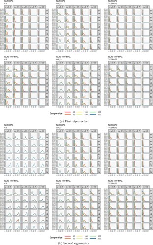
Table 1. Simulation parameters.

Description	Parameter	Values
Population		Normal/Non-normal
Number of variables	p	3, 6, 10, 15, 20, 25
Correlation	ρ	0.1, 0.3, 0.5, 0.7, 0.9
Type of covariance matrix	$\mathbf{\Sigma }$	CS, AR(1), TOEPLITZ
Sample size	n	30, 50, 100, 150, 200, 500

The distribution of AD regarding the first eigenvector varies in location, scale and shape (Figure 1(a)), depending on n, p, ρ and the type of matrix $\mathbf{\Sigma }$, regardless the parent population. First, consider the distribution of AD for a normal population (Figure 1(a)[NORMAL]). Generically, the density of stable solutions is higher when the covariance structure is TOEPLITZ or CS than when is AR(1). In particular, for a TOEPLITZ patterned covariance matrix, the distribution is consistently highly positively skewed, with high probabilities of encountering a stable solution (shaded areas). Higher values of ρ shift to the left the location of the distributions, increasing the (positive) skewness and the probability of encountering a stable solution. This influence is particularly notorious when considering a AR(1) patterned covariance matrix, with the shape of the distribution varying from almost symmetric ($\rho =0.1$) to positively skewed ($\rho =0.9$). The effect of the sample size is particularly notorious when ρ is small. The increase of n also shifts left the location of the distribution and narrows the scale of the distribution, raising the probability of encountering a stable solution. The effect of the number of variables is comparatively less pronounced. However, it is possible to observe that the increase of the number of variables sifts right the location of the distributions, decreasing the probability of encountering a stable solution.

For a non-normal parent population (Figure 1(a)[NON-NORMAL]) we found generically the same results as the described above for a normal parent population. However, the shape of the distribution appears more tailedness, in particular when the covariance matrix is of types CS or AR(1) and for small values of ρ.

The distribution of AD regarding the second eigenvector also varies in location, scale and shape (Figure 1(b)), depending on the values of n, p, ρ and the type of matrix $\mathbf{\Sigma }$, regardless the parent population. The effects are similar to the previously described for the first eigenvector if the covariance matrices are of types AR(1) or TOEPLITZ, regardless the population. However, when the covariance matrix is of type CS (Figure 2(b), [NORMAL][CS] and [NON-NORMAL][CS]), the center of the distribution of the AD of the second eigenvector is higher than the one for the first eigenvector and the distributions range from approximately symmetric to negatively skewed, depending on the values of the parameters. As a consequence, the probability of encountering a stable solution (shaded areas) is zero (or near zero) regardless the values of p, ρ or n. These characteristics are consistently found when the parent population is either normal or non-normal.

Figure 2. QQplots comparing the empirical distribution of the angle between the population and sample eigenvectors under normal and non-normal parent populations as a function of covariance matrix pattern, covariance matrix parameter (ρ) and sample size (n). Shaded area correspond to cosines between 0.95 and 1 (stable solutions). (a) First eigenvector (b) Second eigenvector.

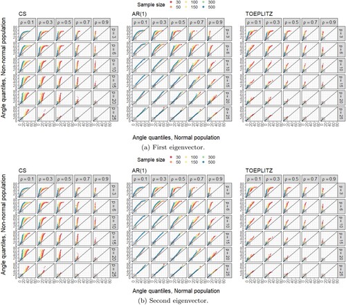
Figure 3. Estimated densities of the global angular displacement as a function of covariance matrix pattern, covariance matrix parameter (ρ) and sample size (n), for both normal and non-normal parent populations. Dashed vertical lines correspond to perfect stability. (a) First 2 principal components ($G_2$) (b) All principal components ($G_p$).

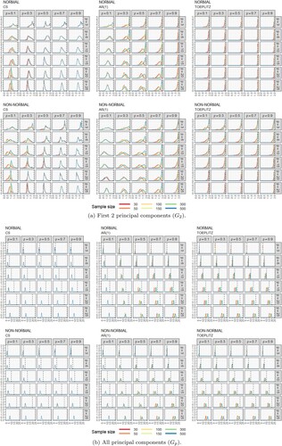
Figure 2 presents the QQplots comparing the distributions of AD between normal and non-normal populations. Generically, Figure 2(a)[CS] shows sets of linearly aligned points lying above and not parallel to the reference line, with the upper end of the plot deviating from the reference line. Hence, in this case, the distributions of AD under normal and non-normal parent populations strongly differ in scale, with lower cumulative probabilities for the same angle values under a non-normal population. For the AR(1) scenario, the plots (Figure 2(a)[AR(1)]) show mainly linearly aligned sets of points either essentially parallel and lying above or coincident with the reference line. Thus, in this case, the distribution of AD under normal and non-normal populations either differ in location, with lower cumulative probabilities for the same angle values under a non-normal population, or agree quite well. For a TOEPLITZ type of covariance (Figure 2(a)[TOEPLITZ]) matrix, with p = 20 or p = 25, the estimated density for a non-normal population is approximately the same estimated for a normal population. However, when $p\le 15$, all plots show sets of points that are not parallel to the reference line. Moreover, the points align linearly above with (positive) slopes higher than the reference line. This fact indicates that the distribution of AD under normal and non-normal parent populations differ in scale, with lower cumulative probabilities for the same angle values under a non-normal population, i.e. lower probability of finding a stable solution. Figure 2(b) presents the QQplots comparing the distributions of AD between normal and non-normal populations, regarding the second eigenvector. Generically, Figure 2(b)[CS] shows a very distint pattern from the one observed in Figure 2(a)[CS]. In this case, the points lie very close to the reference line, indicating minor or negligible differences between the distributions under normal and non-normal populations. The remaining Figure 2(b)[AR(1)] and 2(b)[TOEPLITZ] present patterns essentially identical to the ones described for the first eigenvector.

The estimated probability of having an angle between the first population and sample eigenvectors, whose absolute cosine lies between 0.95 and 1 ($\mathbb{P}(0.95<|\cos ({\theta }_1)|<1)$), was determined based on the distributions depicted in Figure 1. Generically, under a normal parent population, this probability is consistently high or very high (above 0.7 or 0.9, repectively) if the covariance matrix is TOEPLITZ regardless the values of ρ and n. The CS type of covariance structure also ensures very high probabilities of having stable solutions (except if ρ and n are small). The type of covariance AR(1) provides the worst scenario typically with low to very low probabilities of having stable solutions (except if p is small and ρ is high). In summary, as expected, given the described characteristics of the distribution of AD, if the parent population is normal and the covariance matrix is of type TOEPLITZ, then it is very likely to have a stable first PC. For a AR(1) covariance type, the stability of the first PC depends severely on the other studied factors, being hard to achieve with many variables, small samples and low correlations. For a CS covariance type, the stability of the first PC is also harder to achieve with smaller samples and low correlations. When samples are drawn from a non-normal instead of a normal population, given the same conditions, it is less likely to have a stable solution, regardless the value of the remaining parameters. This effect is particularly notorious if p is small (e.g. for p = 3).

The estimated probability of having an angle between the second population and sample eigenvectors, whose absolute cosine lies between 0.95 and 1 ($\mathbb{P}(0.95<|\cos ({\theta }_2)|<1)$), depends greatly on the covariance structure. This probability is zero (or near zero) for a CS covariance matrix, regardless the other studied conditions. If the covariance matrix is of type AR(1), then the stability of the second PC is harder to achieve. Samples from non-normal populations with TOEPLITZ covariance structures may also generate stable second eigenvectors. However, for non-normal parent populations the stability of the second component is much more dependent on the sample size and the correlation value than the stability of the first eigenvector.

Recall that global angular displacement, $G_k$, measures the global stability of the first k axes, serving as an index of subspaces coincidence. Therefore, perfect stability of the two first PC corresponds to $G_2=2$ and perfect global stability to $G_p=p$. Our results show a clear influence of the type of covariance matrix over the stability of the first two PC. When the covariance matrix is of type CS, the mode of the distribution of $G_2$ is consistently different from 2, which indicates a consistent lack of cumulative stability considering the two first PC. However, when the covariance matrix is type AR(1) the mode of the distribution of $G_2$ tends to approximate the value 2, with the increase of ρ (and n). For the covariance matrix TOEPLITZ, the mode of the distribution of $G_2$ coincides with 2 in all the situations. As mentioned, the increase of ρ and n tends to improve the cumulative stability of the first two PC, being particularly notorious if the covariance is AR(1). The effect of the number of variables seems negligible in the sense that does not change the closeness between $G_2$ and the value 2. As expected, global stability (considering all the subspaces) is harder to reach with the increase of p. Again, the increase of ρ and n tends to improve the global stability. Given the same conditions, the values of $G_2$ and $G_p$ tend to be (slightly) higher under a normal than under a non-normal parent population, although this difference tends to narrow and disappear with the increase of ρ and n.

5.2. Stability diagnosis

Our results show that for moderate to highly likely stability conditions ($\mathbb{P}(0.95\le |\cos {\theta }_k|\le 1)>0.4$), there is a well defined linear relationship between $\mathbb{P}(0.95\le |\cos {\theta }_k|\le 1)$ and $se({\ell }_k)/\mathrm{\Delta }{\ell }_k$, for k = 1, 2 (first and second principal components, respectively). As expected, $se({\ell }_1)/\mathrm{\Delta }{\ell }_1$ increases with the decrease of $\mathbb{P}(0.95\le |\cos {\theta }_1|\le 1)$ as unstable solutions are typically associated with smaller eigenvalues spacings, and, therefore, higher ratios. Given a fixed value of $\mathbb{P}(0.95\le |\cos {\theta }_1|\le 1)$, $se({\ell }_1)/\mathrm{\Delta }{\ell }_1$ is higher for non-normal than normal populations. The results obtained for a TOEPLITZ covariance matrix are predominantly stable, therefore associated with low values of $se({\ell }_1)/\mathrm{\Delta }{\ell }_1$.

The results indicate that the second principal component is typically unstable if the covariance matrix is type CS. Hence, in this case, as expected, the average values of $se({\ell }_2)/\mathrm{\Delta }{\ell }_2$ are comparatively high. For the remaining covariance structures, the relation between the ratio $se({\ell }_2)/\mathrm{\Delta }{\ell }_2$ and $\mathbb{P}(0.95\le |\cos {\theta }_2|\le 1)$ is similar to the observed for the first PC.

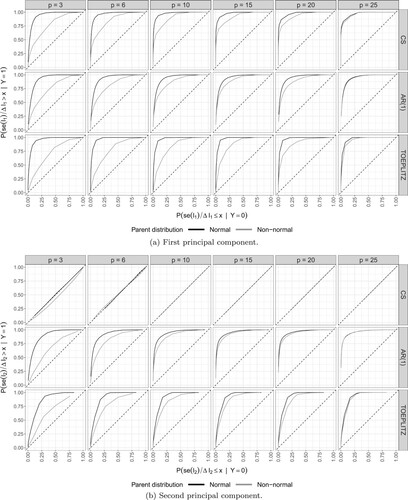
Given these relations, the statistic $se({\ell }_k)/\mathrm{\Delta }{\ell }_k$ was evaluated as a sample criterion for stability, regarding the two first PC. Figure 4 shows the ROC curves for the two first PC. Generically, the stability criterion based on the ratio $se({\ell }_k)/\mathrm{\Delta }{\ell }_k$ performs increasingly better with the increase of the number of variables. The plots also show that this criterion works better if the population is normal than if it is non-normal, although this difference is only relevant when the number of variables is under 15. This sample criterion is nearly a perfect tool for stability diagnosis if p is high. However, it is very clear the degradation of this criterion for k = 2, although depending on the type of covariance matrix. Figure 4(b) shows this degradation for the second principal component when the covariance type is CS. In this case, the statistic in completely uninformative regarding PCA stability.

Figure 4. ROC curves. (a) First principal component (b) Second principal component.

6. Real data examples

In this section we address the problem of PC stability exploring two real datasets. The explored datasets, obtained from the Flury R package [37], encompass information on head measurements of male and female soldiers of the Swiss Army. In allometry studies, like the ones based on these datasets, the first two principal components interpretation are commonly regarded as composite indicators of size or shape when, respectively, the coefficients have all the same sign or include both positive and negative values. Thus, in these cases, stability seems a reasonable requirement to legitimate these interpretations.

The two datasets present sample covariance matrices with relatively different degrees of sphericity with values of approximately 0.8 and 0.9 (equation (1)), respectively. In addition, Mardia test of skewness [38] rejects symmetry for male measurements (p = 0.003) rejecting, therefore, normality. For female measurements both Mardia tests for skweness and kurtosis fail to reject a parent multivariate normality (p = 0.068 and p = 0.304, respectively).

For the described datasets, we evaluated the stability of both the first and second PC using the measure defined by (8(8) $\frac{se({\ell }_k)}{\mathrm{\Delta }{\ell }_k}=\frac{{\ell }_k(2/n{)}^{1/2}}{({\ell }_k-{\ell }_{k+1})}(k=1,\dots ,p-1)$(8) ). Furthermore, bootstrap resampling was used to construct 1000 samples (with replacement), with the same size as the original datasets, and represent bootstrap sampling distribution of (8(8) $\frac{se({\ell }_k)}{\mathrm{\Delta }{\ell }_k}=\frac{{\ell }_k(2/n{)}^{1/2}}{({\ell }_k-{\ell }_{k+1})}(k=1,\dots ,p-1)$(8) ).

Based on these distributions we have calculated the bootstrap percentile confidence intervals. Table 2 summarises, for the two datasets, both the mean point estimate and the 95% percentile bootstrap confidence interval (95%BCI) for the measure (8(8) $\frac{se({\ell }_k)}{\mathrm{\Delta }{\ell }_k}=\frac{{\ell }_k(2/n{)}^{1/2}}{({\ell }_k-{\ell }_{k+1})}(k=1,\dots ,p-1)$(8) ).

Table 2. Stability diagnosis summary (Equation (8(8) $\frac{se({\ell }_k)}{\mathrm{\Delta }{\ell }_k}=\frac{{\ell }_k(2/n{)}^{1/2}}{({\ell }_k-{\ell }_{k+1})}(k=1,\dots ,p-1)$(8) )) applied to Swiss Army real data datasets [37].

	1st PC		2nd PC
Dataset	Mean	95%BCI	Mean	95%BCI
Male soldiers	0.19	[0.15, 0.29]	0.28	[0.18,0.48]
Female soldiers	1.06	[0.33, 3.46]	0.72	[0.33,1.94]

The 95%BCI based on the second dataset is around 27 times wider than the 95%BCI based on the first dataset, reflecting the unstability of the correspondent first PC, regardless the inferred parent normal population. This result is in accordance with the higher degree of sphericity of this dataset. Furthermore, the bootstrap probability of having a value over one in the female dataset is around 0.31 which indicates a quite considerable unstable solution. In contrast, all the estimates in the male dataset are under one.

7. Conclusions

The purpose of this work was to study the conditions under which it is expected to encounter stable principal components with respect to the parent populations pattern, namely regarding the two first PC, as these are frequently targeted either to visualize multivariate datasets on a 2D graphical display or to represent main uncorrelated latent variables. In both situations, principal components analysis is being used to represent the parent population first latent dimensions. This can be done using a PCA as this method provides a new coordinate system that, while retaining as much variability as possible, provides orthogonal principal components, ensuring that the different components are measuring separate dimensions, thus making this technique a seductive candidate to explore parent population latent traits and represent multivariate data in two dimensions.

The results obtained in this study show that, although it is less likely to have unstable solutions when samples are draw from a normal population, this assumption may in fact not be mandatory to obtain a stable PCA solution, being the stability much more dependent on other factors, namely on the covariance matrix (type of structure, dimension and correlation value). Hence, given a parent non-normal population, sample principal components may be stable as long as the covariance structure is not spherical which is achieved more easily with high correlation values according to the order TOEPLITZ > CS > AR(1). The sample size may act as an extra guarantee, in the sense that bigger samples may compensate poor departures from spherical structures, increasing the probability of having stable solutions.

The covariance structure seems to be the major factor in determining PCA stability, as clear non-spherical structures, regardless the parent population and the sample size (being as low as e.g. n = 10), enable to achieve a stable solution. Although the lack of normality seems to be compensated by the sample size, a poor departure from a spherical covariance structure does not seem to be overcome in the same way. In fact, equal or similar eigenvalues, are associated with circular projections, which make difficult to distinguish axes importance. In this situation, because of this degeneracy, i.e. this indistinguishability in terms of eigenvalues, the eigenvectors span a dimensional space in which these orthogonal vectors are arbitrary and therefore cannot be uniquely defined. Conversely, the more distinct the eigenvalues are the less spherical will be the configuration of the points projections in the subspace and more easy it will become to distinguish the components direction in the subspace. Hence, not surprisingly the covariance structure, which determines subspaces degeneracy, appears as the most important feature in determining PC stability. Furthermore, the increase of the number of variables generally increases the probability of having the two first PC stable. However, global stability is harder to reach as the number of variables increases.

The sample criterion for PCA stability defined by (8(8) $\frac{se({\ell }_k)}{\mathrm{\Delta }{\ell }_k}=\frac{{\ell }_k(2/n{)}^{1/2}}{({\ell }_k-{\ell }_{k+1})}(k=1,\dots ,p-1)$(8) ) has shown to be a useful tool for the stability diagnosis regarding the first two PC. Typically high values of this ratio are associated with degenerated subspaces and, therefore, with unstable solutions. Low ratios are indicative of non-degenerated subspaces, i.e. sable solutions.

Acknowledgments

The authors are grateful for the helpful suggestions made by a referee in an initial version of this manuscript.

Disclosure statement

No potential conflict of interest was reported by the author(s).

Additional information

Funding

This work is funded by national funds through the FCT – Fundação para a Ciência e a Tecnologia, I.P., under the scope of the projects UIDB/00297/2020 and UIDP/00297/2020 (Center for Mathematics and Applications).

Notes

1 Defined by an angle ${\theta }_k$, such that $0.95\le |\cos {\theta }_k|\le 1(k=1,\dots ,p)$.

References

- Jolliffe IT. A 50-year personal journey through time with principal component analysis.J Multivar Anal. 2022;188:104820.
- Zamprogno B, Reisen VA, Bondon P, et al. Principal component analysis with autocorrelated data. J Stat Comput Simul. 2020;90(12):2117–2135.
- Jolliffe IT. Principal component analysis. New York: Springer; 2002.
- Shen D, Shen H, Marron JS. A general framework for consistency of principal component analysis. J Mach Learn Res. 2016;17(150):1–34. http://jmlr.org/papers/v17/14-229.html.
- Jolliffe IT, Cadima J. Principal component analysis: a review and recent developments. Philos Trans R Soc A: Mathematical, Physical and Engineering Sciences. 2016;374(2065):20150202.
- Morrison DF. Multivariate statistical methods. Thomson/Brooks/Cole; 2005. (Duxbury advanced series).
- Sprent P. The mathematics of size and shape. Biometrics. 1972;28(1):23–37. http://www.jstor.org/stable/2528959.
- Cadima J, Jolliffe IT. Size- and shape-related principal component analysis. Biometrics. 1996;52(2):710–716. http://www.jstor.org/stable/2532909.
- Somers KM. Allometry, isometry and shape in principal components analysis. Syst Zool. 1989;38(2):169–173. http://www.jstor.org/stable/2992386.
- Kocovsky PM, Adams JV, Bronte CR. The effect of sample size on the stability of principal components analysis of truss-based fish morphometrics. Trans Am Fish Soc. 2009;138(3):487–496.
- Yoo C, Shahlaei M. The applications of PCA in QSAR studies: a case study on CCR5 antagonists. Chem Biol Drug Des. 2017;91(1):137–152.
- Siddig NA, Al-Subhi AM, Alsaafani MA, et al. Applying empirical orthogonal function and determination coefficient methods for determining major contributing factors of satellite sea level anomalies variability in the Arabian Gulf. Arabian J Sci Eng. 2021;47(1):619–628.
- Hannachi A, Jolliffe IT, Stephenson DB. Empirical orthogonal functions and related techniques in atmospheric science: a review. Int J Climatol. 2007;27(9):1119–1152.
- Gauch Jr HG. Noise reduction by eigenvector ordinations. Ecology. 1982;63(6):1643–1649.
- Peres-Neto PR, Jackson DA, Somers KM. How many principal components? Stopping rules for determining the number of non-trivial axes revisited. Comput Statist Data Anal. 2005;49(4):974–997. Available from: https://www.sciencedirect.com/science/ARTICLE/pii/S0167947304002014.
- Gifi A. Nonlinear multivariate analysis. Wiley; 1990. (Wiley series in probability and statistics).
- Daudin J, Duby C, Trecourt P. Stability of principal component analysis studied by the bootstrap method. J Theoretical Appl Statist. 1988;19:241–258.
- Sinha AR, Buchanan BS. Assessing the stability of principal components using regression. Psychometrika. 1995;60(3):355–369.
- Lin L, Higham NJ, Pan J. Covariance structure regularization via entropy loss function. Comput Statist Data Anal. 2014;72:315–327.
- Al-Ibrahim A, Al-Kandari N. Stability of principal components. Comput Stat. 2008;23(1):153–171.
- Dudzinski ML, Norris JM, Chmura JT, et al. Repeatability of principal components in samples: normal and non-normal data sets compared. Multivariate Behav Res. 1975 Jan;10(1):109–117.
- Jackson JE. A user's guide to principal components. Hoboken (NJ): Wiley; 2003. ( Wiley series in probability and statistics).
- Anderson TW. An introduction to multivariate statistical analysis. Wiley; 2003. (Wiley series in probability and statistics).
- Rencher AC. Methods of multivariate analysis. New York: John Wiley & Sons, Inc.; 2002.
- Chan J, Choy B. Analysis of covariance structures in time series. J Data Sci. 2008;6:573–589.
- Littell RC, Pendergast J, Natarajan R. Modelling covariance structure in the analysis of repeated measures data. Stat Med. 2000;19(13):1793–1819.
- Johnson RA, Wichern DW. Applied multivariate statistical analysis. Upper Saddle River: Pearson Prentice Hall; 2007.
- Johnstone IM, Lu AY. On consistency and sparsity for principal components analysis in high dimensions. J Am Stat Assoc. 2009;104(486):682–693. PMID: 20617121, Available from: https://doi.org/10.1198/jasa.2009.0121.
- Quadrelli R, Bretherton CS, Wallace JM. On sampling errors in empirical orthogonal functions. J Clim. 2005;18:3704–3710.
- North GR, Bell TL, Cahalan RF, et al. Sampling errors in the estimation of empirical orthogonal functions. Monthly Weather Rev. 1982;110:699–706.
- Genz A, Bretz F, Miwa T, et al. Mvtnorm: multivariate normal and t distributions; 2019. R package version 1.0-11. Available from: https://CRAN.R-project.org/package=mvtnorm.
- Aitchison J. The statistical analysis of compositional data. GBR: Chapman and Hall, Ltd.; 1986.
- Qu W, Zhang Z. Mnonr: a generator of multivariate non-normal random numbers; 2020. R package version 1.0.0. Available from: https://CRAN.R-project.org/package=mnonr.
- Vale CD, Maurelli VA. Simulating multivariate nonnormal distributions. Psychometrika. 1983 Sep;48(3):465–471.
- Fleishman AI. A method for simulating non-normal distributions. Psychometrika. 1978 Dec;43(4):521–532.
- Tabachnick BG, Fidell LS. Using multivariate statistics. 5th ed. USA: Allyn and Bacon, Inc.; 2006.
- Flury B. Flury: data sets from flury, 1997; 2012. R package version 0.1-3. Available from: https://CRAN.R-project.org/package=Flury.
- Mardia KV, Bibby JM, Kent JT. Multivariate analysis. 1979. Available from: http://www.loc.gov/catdir/toc/els031/79040922.html.