Maximum leave-one-out likelihood method for the location parameter of variance gamma distribution with unbounded density

Abstract

Maximum likelihood estimation of a location parameter fails when the density has unbounded mode. An alternative approach is considered by leaving out a data point to avoid the unbounded density in the full likelihood. This modification gives rise to the leave-one-out (LOO) likelihood. We propose an expectation-conditional maximisation (ECM) algorithm to estimate parameters of variance gamma (VG) distribution with unbounded density by maximising the LOO likelihood. VG distribution has normal mean-variance mixtures representation that facilitates ECM algorithm. K Podgórski, J Wallin [Maximizing leave-one-out likelihood for the location parameter of unbounded densities. Ann Inst Stat Math. 2015;67(1):19–38.] showed that the location parameter estimate which maximises the LOO likelihood is consistent and super-efficient. In the case of repeated data, the LOO likelihood is still unbounded and we extend it to Weighted LOO (WLOO) likelihood. We perform simulations to investigate the accuracy of ECM method using WLOO likelihood and compare it with other likelihood methods, including the alternating ECM with fixed and adaptive caps to the unbounded density, the ghyp package using multi-cycle ECM, and the ECM using LOO likelihood. Lastly, we explore the asymptotic properties of the location parameter estimate of VG distribution such as the optimal convergence rate and asymptotic distribution.

Keywords:

• Unbounded likelihood
• leave-one-out likelihood
• variance gamma distribution
• ECM algorithm
• asymptotic distribution

1. Introduction

Asymptotic properties of maximum likelihood estimation for location parameters have been studied for the case when the likelihood is non-differentiable but bounded [1]. However, this method breaks down when the likelihood is unbounded at certain points. Alternative methods for the unbounded density case have been considered in Refs [2,3] and in Ref. [4] where they proved consistency of the location estimate using the Bayesian approach.

Under the likelihood approach however, modifications to the full likelihood are necessary since the unbounded points occur at the data points. A possible solution is to leave out a data point closest to the location parameter in the full likelihood. This modification leads to a concept known as the leave-one-out (LOO) likelihood proposed by Podgórski and Wallin [5]. They proved consistency and super-efficiency of the location estimate that maximises the LOO likelihood when the density is unbounded. More precisely, under certain regularity conditions, they found an upper bound for the index of convergence rate for the location parameter estimate (see Section 3.2 for the definition of convergence rate and its index). Currently, there are no theoretical results regarding the optimal convergence rate and the asymptotic distribution of the maximum LOO likelihood estimate for the location parameter when the density is unbounded or with cusp. Since the theoretical derivation of these two asymptotic properties is very challenging, we propose to perform numerical simulations to investigate the properties and obtain some insights for the theoretical development.

To demonstrate the idea, we consider multivariate skewed variance gamma (VG) distributions with unbounded densities when the shape parameters $\nu \le d/2$ where d is the dimension of the multivariate data. To estimate the parameters of VG distributions with unbounded densities, Nitithumbundit and Chan [6] proposed an expectation-conditional maximisation (ECM) algorithm [7] where they proposed to cap the density within a small interval of the location parameter. Depending on whether the conditional density or actual density is used to estimate the shape parameter, ECM algorithm can be further classified into multi-cycle ECM (MCECM) and ECM either (ECME) [8,9]. In this paper, the ECME algorithm is still called ECM algorithm as the methodological idea of ECME is similar to ECM. However, a drawback to capping the unbounded density is that the size of the interval to cap the density is somewhat arbitrary, and that different intervals can give different results. Podgórski and Wallin [5] established a theoretical framework for using the LOO likelihood in an expectation-maximisation (EM) algorithm to estimate the location parameter of univariate symmetric generalised Laplace distribution (which is equivalent to VG distribution proposed by Madan and Seneta [10]) with fixed shape parameter and unbounded density.

However, when there are data multiplicity (repeated data), the LOO likelihood will still be unbounded even if we leave out one of the data points. If we leave out multiple data points to obtain the leave-multiple-out (LMO) likelihood, this LMO likelihood has varied data size and contribution across the parameter space depending on the data multiplicities. This inconsistent data contribution leads to a discontinuous LMO likelihood. It is necessary to address this data multiplicity issue in the LOO likelihood as the issue is likely to occur for three reasons. Firstly, data rounding is common in practice simply for convenience or for reducing data storage. Secondly, as big data are more prevalence in recent years, the chance of data multiplicity increases with sample size. Lastly, as measurements are made more instantaneously for high-frequency data, the changes between measurements will be minimal and hence measures using these changes such as returns will be extremely small or even zero again giving rise to data multiplicity. Although the chance of data multiplicity is lower when the means for the time series model say change over time and when multi-dimensional models are used, one will never be sure in practice if data multiplicity exists. Hence, it is always advisable to fix the LOO likelihood issues to provide numerically stable estimates.

Following this idea, Nitithumbundit and Chan [11] proposed weighted LOO (WLOO) likelihood to deal with discontinuous LMO likelihood when there are data multiplicities. They applied WLOO likelihood to multivariate data with unbounded densities and derived an ECM algorithm [8] to obtain the maximum WLOO estimate of the location parameters of the vector autoregressive moving average (VARMA) model with multivariate skewed VG distribution when densities are cusped or unbounded with respect to the location parameters. The proposed algorithm is an extension of the EM algorithm. They derive explicit formulae to calculate all parameters in the expectation step (E-step) and conditional maximisation steps (CM-steps). When there are data multiplicities, they applied WLOO likelihood to obtain a continuous likelihood function. However, the paper focuses on the application and did not study the properties of this new method using the ECM algorithm with WLOO likelihood.

The objective of this paper is to fill up this research gap and study the properties of our proposed ECM algorithm with WLOO likelihood. Our first objective assesses the accuracy of the ECM algorithm using LOO likelihood in the case of no data multiplicity and compare the ECM algorithm using the LOO and WLOO likelihoods with other full likelihood methods in the case of data multiplicity due to repetition and rounding. To focus on the properties of the method, we make two modifications to Ref. [11]. We consider a constant mean instead of the ARMA mean and we drop the alternating ECM (AECM) algorithm which aims only to improve the convergence rate of the ECM algorithm. Our second and main objective analyses the asymptotic behaviour including the optimal convergence rate and asymptotic distribution for the maximum LOO likelihood estimate for the location parameter through simulation studies using data simulated from the VG distribution with different sample sizes and shape parameters. Specifically, we investigate how the index of optimal convergence rate in Ref. [5] for the location parameter estimates and its asymptotic distribution change across the shape parameter of VG distribution with unbounded or cusp density. From these studies, we aim to approximate the asymptotic distribution with some distributions to provide standard error for the location parameter estimates.

We choose VG distribution to demonstrate the ability of our proposed methods to deal with unbounded densities for three important reasons. Firstly, VG distribution is an important special case of the more general class, the generalised hyperbolic (GH) distribution [12]. When GH distribution approaches VG distribution, one of its shape parameters will approach the boundary of the parameter space potentially causing the density to become unbounded. Although Protassov [13] proposed an EM algorithm for GH distribution, such algorithm considers only regular shape parameters inside the parameter space and hence it does not truly capture the case of VG distribution with unbounded density when one of the shape parameter approaches the boundary of the parameter space causing unbounded densities. Our proposed ECM algorithm deals with such a case when the density is unbounded. Secondly, VG distribution has a normal mean-variance mixture (NMVM) representation that facilitates the implementation of ECM algorithm. Lastly, VG distribution has applications in many areas such as finance, signal processing and quality control. See Ref. [14] for other applications and further details on generalised Laplace distribution. We remark that the idea of the proposed ECM algorithm can be applied to other distributions in NMVM representation including Student's t and GH distributions with some suitable adjustments in the E-step.

The remaining paper is organised as follows. Section 2 summarises some important properties of the multivariate skewed VG distribution. Section 3 formulates the maximum LOO likelihood framework for estimating the location parameter of distributions with unbounded densities, reports some properties of the estimate and introduces the WLOO likelihood with two examples to explain the weight settings. Section 4 introduces the ECM algorithm using the LOO and WLOO likelihoods to estimate parameters from the VG distribution. Although the methodologies in Sections 3 and 4 were described in Ref. [11], we present them in a slightly different way starting with defining different LOO likelihoods which are the focus and with different emphasis giving more technical details. Moreover, some equations are modified for the different mean structures. Section 5 presents three simulation studies. The first study tests the accuracy of our ECM method using WLOO likelihood while the second study compares the accuracy of the ECM method with other full and LOO likelihood methods in three scenarios, namely, no data multiplicity, data multiplicity due to repetition and data multiplicity due to rounding. The last study analyses the asymptotic behaviour of the maximum LOO likelihood method to estimate the location parameter of VG distribution. Section 6 concludes the paper with further remarks.

2. Variance gamma distribution

The probability density function (pdf) of a d-dimensional VG distribution is given by (1) $f_{\mathrm{V}\mathrm{G}}\left(\mathit{y}\right)=\frac{2^{1-\frac{d}{2}}{\nu }^{\nu }}{{\left|\mathbf{\Sigma }\right|}^{\frac{1}{2}}{\pi }^{\frac{d}{2}}\mathrm{\Gamma }\left(\nu \right)}\frac{K_{\nu -\frac{d}{2}}\left(\sqrt{[2\nu +{\mathit{\gamma }}^{\mathrm{\top }}{\mathbf{\Sigma }}^{-1}\mathit{\gamma }]}z\right)\exp \left(\right(\mathit{y}-\mathit{\mu }{)}^{\mathrm{\top }}{\mathbf{\Sigma }}^{-1}\mathit{\gamma })}{(2\nu +{\mathit{\gamma }}^{\mathrm{\top }}{\mathbf{\Sigma }}^{-1}\mathit{\gamma }{)}^{\frac{1}{4}(2\nu -d)}{z}^{\frac{1}{2}(d-2\nu )}}$(1) where $z^2=(\mathit{y}-\mathit{\mu }{)}^{\mathrm{\top }}{\mathbf{\Sigma }}^{-1}(\mathit{y}-\mathit{\mu })$, $\mathit{\mu }\in {\mathbb{R}}^d$ is the location parameter, $\mathbf{\Sigma }$ is a $d\times d$ positive definite symmetric scale matrix, $\mathit{\gamma }\in {\mathbb{R}}^d$ is the skewness parameter, $\nu >0$ is the shape parameter, $\mathrm{\Gamma }(\cdot )$ is the gamma function and $K_{\lambda }(\cdot )$ is the modified Bessel function of the second kind with index λ [15].

The VG distribution has a normal mean-variance mixtures representation [12] given by (2) $\mathit{y}|u\sim {\mathcal{N}}_d(\mathit{\mu }+\mathit{\gamma }u,u\mathbf{\Sigma }),u\sim \mathcal{G}(\nu ,\nu )$(2) where $\mathcal{G}(a,b)$ is a Gamma distribution with shape parameter a>0, rate parameter b>0 and pdf $f_{\mathrm{G}}\left(u\right)=\frac{b^a}{\mathrm{\Gamma }\left(a\right)}{u}^{a-1}\exp (-bu),\mathrm{f}\mathrm{o}\mathrm{r}u>0.$The mean and covariance matrix of a VG random vector $\mathit{Y}$ are given by $\mathbb{E}\left(\mathit{Y}\right)=\mathit{\mu }+\mathit{\gamma }\mathrm{a}\mathrm{n}\mathrm{d}\text{cov}\left(\mathit{Y}\right)=\mathbf{\Sigma }+\frac{1}{\nu }\mathit{\gamma }{\mathit{\gamma }}^{\mathrm{\top }},$respectively. As $\mathit{y}\to \mathit{\mu }$, the pdf in (1(1) $f_{\mathrm{V}\mathrm{G}}\left(\mathit{y}\right)=\frac{2^{1-\frac{d}{2}}{\nu }^{\nu }}{{\left|\mathbf{\Sigma }\right|}^{\frac{1}{2}}{\pi }^{\frac{d}{2}}\mathrm{\Gamma }\left(\nu \right)}\frac{K_{\nu -\frac{d}{2}}\left(\sqrt{[2\nu +{\mathit{\gamma }}^{\mathrm{\top }}{\mathbf{\Sigma }}^{-1}\mathit{\gamma }]}z\right)\exp \left(\right(\mathit{y}-\mathit{\mu }{)}^{\mathrm{\top }}{\mathbf{\Sigma }}^{-1}\mathit{\gamma })}{(2\nu +{\mathit{\gamma }}^{\mathrm{\top }}{\mathbf{\Sigma }}^{-1}\mathit{\gamma }{)}^{\frac{1}{4}(2\nu -d)}{z}^{\frac{1}{2}(d-2\nu )}}$(1) ) is given by (3) $\begin{array}{r}{f}_{\mathrm{V}\mathrm{G}}\left(\mathit{y}\right)\sim \{\begin{array}{ll}{2}^{\nu -d}{\pi }^{-\frac{d}{2}}{\left|\mathbf{\Sigma }\right|}^{-\frac{1}{2}}\frac{\mathrm{\Gamma }(\nu -\frac{d}{2})}{\mathrm{\Gamma }\left(\nu \right)}\frac{{\nu }^{\nu }}{(2\nu +{\mathit{\gamma }}^{\mathrm{\top }}{\mathbf{\Sigma }}^{-1}\mathit{\gamma }{)}^{\frac{2\nu -d}{2}}}& \mathrm{i}\mathrm{f}\nu >\frac{d}{2},\\ -2^{1-d}{\pi }^{-\frac{d}{2}}{\left|\mathbf{\Sigma }\right|}^{-\frac{1}{2}}\frac{d^{\frac{d}{2}}}{\mathrm{\Gamma }\left(\frac{d}{2}\right)}\log \left(z\right)& \mathrm{i}\mathrm{f}\nu =\frac{d}{2},\\ 2^{-\nu }{\pi }^{-\frac{d}{2}}{\left|\mathbf{\Sigma }\right|}^{-\frac{1}{2}}\frac{\mathrm{\Gamma }(\frac{d}{2}-\nu )}{\mathrm{\Gamma }\left(\nu \right)}{\nu }^{\nu }{z}^{2\nu -d}& \mathrm{i}\mathrm{f}\nu <\frac{d}{2}.\end{array}\end{array}$(3) Hence the density becomes unbounded at $\mathit{\mu }$ when $\nu \le \frac{d}{2}$. This poses some technical difficulty when working with VG distribution as it is unclear whether the shape parameter will fall into the unbounded range. It is also worth noting that the density is bounded with a cusp when $\frac{d}{2}<\nu \le \frac{d+1}{2}$.

This problem of unbounded density is illustrated in Figure 1 of Ref. [11] with the full log-likelihood and LOO log-likelihood across the location parameter for a data of 10 observations simulated from a standard VG distribution ($\mu =0$, $\sigma =1$, $\gamma =0$) with shape parameter $\nu =0.2$. Leaving the data point out essentially smooths out the unbounded log-likelihood at data points so the maximum can be well-defined. Additionally, if we zoom in at around $\mu =0$, we observe that cusps tend to occur between data points.

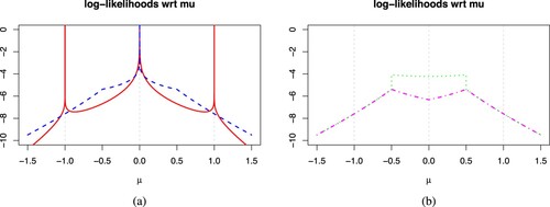
Figure 1. Plots of full (solid red), LOO (striped blue), LMO (dotted green), and WLOO (dot & striped magenta) log-likelihoods of univariate symmetric VG distribution with $\nu =0.4$ for data set $\{-1,0,1,0\}$ represented by light grey vertical strips. (a) Full and LOO log-likelihoods and (b) LMO and WLOO log-likelihoods.

3. Maximum leave-one-out likelihood

Let $\mathit{y}=({\mathit{y}}_1,\dots ,{\mathit{y}}_n)$ be observed data from VG distribution with corresponding missing parameters $\mathit{u}=(u_1,\dots ,u_n)$, and $\mathit{\theta }=(\mathit{\mu },\mathbf{\Sigma },\mathit{\gamma },\nu )$ be parameters from VG distribution in parameter space $\mathbf{\Theta }$. The density of the VG distribution is unbounded at $\mathit{\mu }$ when $\nu \le \frac{d}{2}$. Consequently the maximum likelihood estimate is not well-defined since there are multiple unbounded points at each data point in the likelihood function. Kawai [16] showed that for the univariate case, the Fisher information matrix with respect to μ is also not well-defined when $\nu <1/2$. That is if $\nu <1/2$, then ${\mathbb{E}}_{\mathit{\theta }}\left[{(\frac{\mathrm{\partial }}{\mathrm{\partial }\mu }\log f(Y;\mathit{\theta }\left)\right)}^2\right]=\mathrm{\infty }$where Y is a univariate VG random variable with density function f, and the expectation is taken with respect to Y which depends on $\mathit{\theta }$.

We aim to provide a methodology to estimate parameters from VG distribution that can also deal with unbounded density. We first redefine the likelihood so that the maximum is well-defined even with the unbounded density.

3.1. Leave-one-out likelihood

Podgórski and Wallin [5] proposed the observed LOO likelihood to be defined as $L^{\mathrm{L}\mathrm{O}\mathrm{O}}(\mathit{\theta };\mathbf{y})=\prod _{t\ne \kappa \left(\mathit{\mu }\right)}f\left({\mathit{y}}_t\right)$where the LOO index is defined as (4) $\kappa \left(\mathit{\mu }\right)=\underset{t\in \{1,\cdots ,n\}}{\mathrm{a}\mathrm{r}\mathrm{g}\mathrm{m}\mathrm{i}\mathrm{n}}({\mathit{y}}_t-\mathit{\mu }{)}^{\mathrm{\top }}{\mathbf{\Sigma }}^{-1}({\mathit{y}}_t-\mathit{\mu }).$(4) For the case where there are more than one indices, we choose the smallest index. Note that we slightly modify the convention in Ref. [5]: ‘if there are two indices we take the one for which corresponding $y_{k\left(\mu \right)}$ is on the right side of μ’ as it only deals with the univariate case and cannot be easily extended to multivariate setting using this convention. Let the observed LOO log-likelihood be defined as (5) ${\ell }^{\mathrm{L}\mathrm{O}\mathrm{O}}(\mathit{\theta };\mathit{y})=\log L^{\mathrm{L}\mathrm{O}\mathrm{O}}(\mathit{\theta };\mathit{y}).$(5) We remark that when considering asymmetric distributions, the LOO likelihood function is discontinuous. For the VG distribution with skewness, the discontinuity is not an issue since the density is asymptotically symmetric as $\mathit{y}\to \mathit{\mu }$ from (3(3) $\begin{array}{r}{f}_{\mathrm{V}\mathrm{G}}\left(\mathit{y}\right)\sim \{\begin{array}{ll}{2}^{\nu -d}{\pi }^{-\frac{d}{2}}{\left|\mathbf{\Sigma }\right|}^{-\frac{1}{2}}\frac{\mathrm{\Gamma }(\nu -\frac{d}{2})}{\mathrm{\Gamma }\left(\nu \right)}\frac{{\nu }^{\nu }}{(2\nu +{\mathit{\gamma }}^{\mathrm{\top }}{\mathbf{\Sigma }}^{-1}\mathit{\gamma }{)}^{\frac{2\nu -d}{2}}}& \mathrm{i}\mathrm{f}\nu >\frac{d}{2},\\ -2^{1-d}{\pi }^{-\frac{d}{2}}{\left|\mathbf{\Sigma }\right|}^{-\frac{1}{2}}\frac{d^{\frac{d}{2}}}{\mathrm{\Gamma }\left(\frac{d}{2}\right)}\log \left(z\right)& \mathrm{i}\mathrm{f}\nu =\frac{d}{2},\\ 2^{-\nu }{\pi }^{-\frac{d}{2}}{\left|\mathbf{\Sigma }\right|}^{-\frac{1}{2}}\frac{\mathrm{\Gamma }(\frac{d}{2}-\nu )}{\mathrm{\Gamma }\left(\nu \right)}{\nu }^{\nu }{z}^{2\nu -d}& \mathrm{i}\mathrm{f}\nu <\frac{d}{2}.\end{array}\end{array}$(3) ), and so the effect of the discontinuities is minimised for larger sample size. On the other hand, when using other distributions with different skewness behaviour, the LOO index can alternatively be defined as (6) $\kappa \left(\mathit{\mu }\right)=\underset{t\in \{1,\cdots ,n\}}{\mathrm{a}\mathrm{r}\mathrm{g}\mathrm{m}\mathrm{a}\mathrm{x}}f({\mathit{y}}_t;\mathit{\theta }).$(6) In this paper, we adopt the LOO index in (6(6) $\kappa \left(\mathit{\mu }\right)=\underset{t\in \{1,\cdots ,n\}}{\mathrm{a}\mathrm{r}\mathrm{g}\mathrm{m}\mathrm{a}\mathrm{x}}f({\mathit{y}}_t;\mathit{\theta }).$(6) ) and define the maximum LOO likelihood estimate denoted as ${\hat{\mathit{\theta }}}_n^{\mathrm{M}\mathrm{L}\mathrm{L}\mathrm{E}}$ (or simply ${\hat{\mathit{\theta }}}_n$) to be the estimate that maximises the LOO likelihood with respect to $\mathit{\theta }$. This new and more general index definition makes the LOO likelihood continuous and for the symmetric case it would coincide with (4(4) $\kappa \left(\mathit{\mu }\right)=\underset{t\in \{1,\cdots ,n\}}{\mathrm{a}\mathrm{r}\mathrm{g}\mathrm{m}\mathrm{i}\mathrm{n}}({\mathit{y}}_t-\mathit{\mu }{)}^{\mathrm{\top }}{\mathbf{\Sigma }}^{-1}({\mathit{y}}_t-\mathit{\mu }).$(4) ).

3.2. Properties of the maximum leave-one-out likelihood method

For the one-dimensional case, some properties of the location parameter estimate ${\hat{\mu }}_n$ such as consistency and super-efficient rate of convergence are proved by Podgórski and Wallin [5]. We state both the assumptions and theorem relating to these main properties:

(A1)	The pdf $f\left(y\right)=p\left(y\right)|y{|}^{\alpha }$, $\alpha \in (-1,0)$, p has bounded derivative on $\mathbb{R}\mathrm{\setminus }\left\{0\right\}$ and, for some $ϵ>0$, f is non-zero and continuous either on $[-ϵ,0]$ or on $[0,ϵ]$.
(A2)	There exist $\rho >0$ such that $f\left(y\right)=O\left(|y{|}^{-\rho -1}\right)$ when $|y|\to \mathrm{\infty }$.
(A3)	For all $ϵ>0$, the incomplete Fisher information is finite. That is, ${\mathcal{I}}_{ϵ}\left(\mathit{\theta }\right):={\mathbb{E}}_{\mathit{\theta }}[{(\frac{\mathrm{\partial }}{\mathrm{\partial }\mathit{\theta }}\log f(Y;\mathit{\theta }\left)\right)}^2||Y|>ϵ]<\mathrm{\infty }.$

Theorem 3.1

Let f satisfies the assumptions (A1) to (A3) and let $\hat{\mu }$ be the maximizer of $L^{\mathrm{L}\mathrm{O}\mathrm{O}}(\mu ;\mathit{y})$. Then $\hat{\mu }$ is consistent estimate of μ and for any $\text{β}<1/(1+\alpha )$, $n^{\text{β}}({\hat{\mu }}_n-\mu )\stackrel{p}{\to }0$where α is defined in (A1) and $\stackrel{p}{\to }$ means convergence in probability.

This theorem states the lower bound $n^{-\text{β}}$ for the convergence rate of the location parameter estimate using maximum LOO likelihood. For univariate VG distribution, $\alpha =2\nu -1$. Hence setting $\text{β}=1/(1+\alpha )=1/\left(2\nu \right)$ possibly gives us the index for the optimal convergence rate (or the proposed optimal rate) for $\nu <1/2$. Additionally, $n^{\text{β}}({\hat{\mu }}_n-\mu )$ may converge to some asymptotic distribution for some suitable choice of β. We will investigate the asymptotic properties later in Section 5 using simulations from VG distribution.

3.3. Extension to weighted LOO likelihood for data multiplicity

Data multiplicity is common when the measurements have limited level of accuracy. In this case, the LOO likelihood is first extended to the leave-multiple-out (LMO) likelihood defined as $L^{\mathrm{L}\mathrm{M}\mathrm{O}}(\mathit{\theta };\mathit{y})=\prod _{t\ne \mathcal{K}\left(\mathit{\mu }\right)}f({\mathit{y}}_t;\mathit{\theta })$where (7) $\mathcal{K}\left(\mathit{\mu }\right)=\{t\in \{1,\dots ,n\}|{\mathit{y}}_t={\mathit{y}}_{k\left(\mathit{\mu }\right)}\}$(7) represents the LMO indices which correspond to the data points identical to ${\mathit{y}}_{\kappa \left(\mathit{\mu }\right)}$, and $\kappa \left(\mathit{\mu }\right)$ represents the LOO index defined in (4(4) $\kappa \left(\mathit{\mu }\right)=\underset{t\in \{1,\cdots ,n\}}{\mathrm{a}\mathrm{r}\mathrm{g}\mathrm{m}\mathrm{i}\mathrm{n}}({\mathit{y}}_t-\mathit{\mu }{)}^{\mathrm{\top }}{\mathbf{\Sigma }}^{-1}({\mathit{y}}_t-\mathit{\mu }).$(4) ) in Section 3.1. When there are no data multiplicities, the LMO likelihood reduces to the LOO likelihood with consistent $(n-1)$ data contribution. However, when there are varied data multiplicities, the number of data points to leave out is not fixed and so the LMO likelihood has varied data contribution across the parameter space. This inconsistent data contribution throughout the parameter space leads to a discontinuous LMO likelihood. To remedy this, we propose to adjust the LMO likelihood to weighted LOO (WLOO) likelihood defined as (8) $L^{\mathrm{W}\mathrm{L}\mathrm{O}\mathrm{O}}(\mathit{\theta };\mathbf{\text{y}})=\prod _{t=1}^{n}f({\mathit{y}}_t;\mathit{\theta }{)}^{w_t}$(8) where we choose the weights to be (9) $\begin{array}{rl}{w}_t& =\{\begin{array}{ll}0,& \mathrm{i}\mathrm{f}t\in \mathcal{K}\left(\mathit{\mu }\right)\\ \frac{|\mathcal{K}\left(\mathit{\mu }\right)|+|\mathcal{J}\left(\mathit{\mu }\right)|-1}{|\mathcal{J}\left(\mathit{\mu }\right)|},& \mathrm{i}\mathrm{f}t\in \mathcal{J}\left(\mathit{\mu }\right)\\ 1,& \mathrm{o}\mathrm{t}\mathrm{h}\mathrm{e}\mathrm{r}\mathrm{w}\mathrm{i}\mathrm{s}\mathrm{e},\end{array}\end{array}$(9) $\mathcal{K}\left(\mathit{\mu }\right)$ is defined in (7(7) $\mathcal{K}\left(\mathit{\mu }\right)=\{t\in \{1,\dots ,n\}|{\mathit{y}}_t={\mathit{y}}_{k\left(\mathit{\mu }\right)}\}$(7) ) such that $|\mathcal{K}\left(\mathit{\mu }\right)|$ represents the cardinality of the set $\mathcal{K}\left(\mathit{\mu }\right)$, (10) $\mathcal{J}\left(\mathit{\mu }\right)=\{t\in \{1,\dots ,n\left\}\mathrm{\setminus }\mathcal{K}\right(\mathit{\mu }):{\mathit{y}}_t={\mathit{y}}_{j\left(\mathit{\mu }\right)}\}$(10) and $j\left(\mathit{\mu }\right)=\underset{t\in I\mathrm{\setminus }\mathcal{K}\left(\mathit{\mu }\right)}{\mathrm{a}\mathrm{r}\mathrm{g}\mathrm{m}\mathrm{i}\mathrm{n}}({\mathit{y}}_t-\mathit{\mu }{)}^{\mathrm{\top }}{\mathbf{\Sigma }}^{-1}({\mathit{y}}_t-\mathit{\mu })$represents the secondary LOO index for VG distribution in NMVM representation. Similarly, the WLOO log-likelihood is defined as (11) ${\ell }^{\mathrm{W}\mathrm{L}\mathrm{O}\mathrm{O}}(\mathit{\theta };\mathbf{\text{y}})=\sum _{t=1}^n{w}_{t}f({\mathit{y}}_t;\mathit{\theta }).$(11) Clearly, LOO likelihood is the special case of WLOO likelihood when there is no data multiplicity and the weights are chosen to be $w_t=1$. We use two examples with data multiplicity at one and two locations respectively to demonstrate how the weights in (9(9) $\begin{array}{rl}{w}_t& =\{\begin{array}{ll}0,& \mathrm{i}\mathrm{f}t\in \mathcal{K}\left(\mathit{\mu }\right)\\ \frac{|\mathcal{K}\left(\mathit{\mu }\right)|+|\mathcal{J}\left(\mathit{\mu }\right)|-1}{|\mathcal{J}\left(\mathit{\mu }\right)|},& \mathrm{i}\mathrm{f}t\in \mathcal{J}\left(\mathit{\mu }\right)\\ 1,& \mathrm{o}\mathrm{t}\mathrm{h}\mathrm{e}\mathrm{r}\mathrm{w}\mathrm{i}\mathrm{s}\mathrm{e},\end{array}\end{array}$(9) ) are derived to ensure bounded and continuous likelihood as well as consistent weighted data size, that is $\sum _{t=1}^n{w}_t=n-1$, when data with different multiplicities are removed. We call the first example symmetric since there are equal number of data points on each side of the data with multiplicity. The second example is asymmetric as there are different number of data points on each side of the data with multiplicity. In these two examples, the shape parameter $\nu =0.4$ that corresponds to unbounded likelihood. When the density function is skewed, both LOO and WLOO likelihoods are not continuous between data points. Nevertheless, the pdf in (3(3) $\begin{array}{r}{f}_{\mathrm{V}\mathrm{G}}\left(\mathit{y}\right)\sim \{\begin{array}{ll}{2}^{\nu -d}{\pi }^{-\frac{d}{2}}{\left|\mathbf{\Sigma }\right|}^{-\frac{1}{2}}\frac{\mathrm{\Gamma }(\nu -\frac{d}{2})}{\mathrm{\Gamma }\left(\nu \right)}\frac{{\nu }^{\nu }}{(2\nu +{\mathit{\gamma }}^{\mathrm{\top }}{\mathbf{\Sigma }}^{-1}\mathit{\gamma }{)}^{\frac{2\nu -d}{2}}}& \mathrm{i}\mathrm{f}\nu >\frac{d}{2},\\ -2^{1-d}{\pi }^{-\frac{d}{2}}{\left|\mathbf{\Sigma }\right|}^{-\frac{1}{2}}\frac{d^{\frac{d}{2}}}{\mathrm{\Gamma }\left(\frac{d}{2}\right)}\log \left(z\right)& \mathrm{i}\mathrm{f}\nu =\frac{d}{2},\\ 2^{-\nu }{\pi }^{-\frac{d}{2}}{\left|\mathbf{\Sigma }\right|}^{-\frac{1}{2}}\frac{\mathrm{\Gamma }(\frac{d}{2}-\nu )}{\mathrm{\Gamma }\left(\nu \right)}{\nu }^{\nu }{z}^{2\nu -d}& \mathrm{i}\mathrm{f}\nu <\frac{d}{2}.\end{array}\end{array}$(3) ) is approximately symmetric as $\mathit{\mu }$ approaches any data point. So by having more data points, the effect of discontinuities due to skewness is negligible.

Example 1: data multiplicity at a single location

The first data $\{-1,0,1,0\}$ have data multiplicity at a single location 0. Figure 1 plots the LOO log-likelihood across μ. In Figure 2(a), the LOO log-likelihood is unbounded at 0 even after leaving out one data point 0.

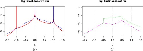
Figure 2. Plot of the full (solid red), LOO (striped blue), LMO (dotted green), and WLOO (dot & striped magenta) log-likelihoods of symmetric VG distribution with $\nu =0.4$ for data set $\{-1,0,1,0,0,1\}$ represented by light grey vertical strips. (a) Full and LOO log-likelihoods and (b) LMO and WLOO log-likelihoods.

The LMO log-likelihood in Figure 2(b) is bounded after leaving out multiple data points at 0 but it also produces discontinuities at the midpoints of $-0.5$ and 0.5. We aim to choose the weights in the WLOO log-likelihood ${\ell }^{\mathrm{W}\mathrm{L}\mathrm{O}\mathrm{O}}\left(\mu \right)=w_1\log f(-1)+2w_2\log f\left(0\right)+w_3\log f\left(1\right)$($w_2=w_4$) to ensure consistent data contribution, that is, $\sum _{t=1}^n{w}_t=n-1$. Since the pdf is assumed to be symmetric, we define $g_t(|y_t-\mu |)=f(y_t;\mu )$and analyse the WLOO log-likelihood around the small neighbourhood $ϵ>0$ of the midpoints located at $-0.5$ and 0.5. It is sufficient to look at one of the midpoints.

Midpoint of 0 and 1: At $\mu =0.5+ϵ$, the data point $y_3=1$ is closest to μ. So we leave out $y_3=1$ in the WLOO log-likelihood by setting $w_3=0$. This gives us ${\ell }^{\mathrm{W}\mathrm{L}\mathrm{O}\mathrm{O}}(0.5+ϵ)=w_1\log g_1(1.5+ϵ)+2w_2\log g_2(0.5+ϵ)+0\log g_3(0.5-ϵ).$Since the data point $y_1=-1$ has a single contribution to the log-likelihood, we set $w_1=1$ leaving the other weights $w_2=w_4=1$ so that $\sum _{t=1}^4{w}_t=3$. At $\mu =0.5-ϵ$, the data points $x_2=x_4=0$ is closest to μ so we set $w_2=0$ which gives us ${\ell }^{\mathrm{W}\mathrm{L}\mathrm{O}\mathrm{O}}(0.5-ϵ)=w_1\log g_1(1.5-ϵ)+0\log g_2(0.5-ϵ)+w_3\log g_3(0.5+ϵ).$Again, we set $w_1=1$ leaving $w_3=2$ so that $\sum _{t=1}^4{w}_t=3$. Choosing these weights gives us a continuous WLOO likelihood at $\mu =0.5$ given by ${\ell }^{\mathrm{W}\mathrm{L}\mathrm{O}\mathrm{O}}\left(0.5\right)=\log g_1\left(1.5\right)+2\log g_2\left(0.5\right)$where $g_2(|0-0.5|)=g_3(|1-0.5|)$. This shows that after leaving out multiple data points, extra weight is added to the neighbouring data points to compensate for the missing weights.

Example 2: data multiplicities at two locations

The second data $\{-1,0,1,0,0,1\}$ have different data multiplicities at 0 and 1. As before we define the WLOO log-likelihood as ${\ell }^{\mathrm{W}\mathrm{L}\mathrm{O}\mathrm{O}}\left(\mu \right)=w_1\log f(-1)+3w_2\log f\left(0\right)+2w_3\log f\left(1\right).$

Midpoint of -1 and 0: At $\mu =-0.5-ϵ$, we set $w_1=0$ giving $w_2=w_3=1$ whereas at $\mu =-0.5+ϵ$, we set $w_2=0$ giving $w_1=w_3=1$. Hence the WLOO log-likelihood is ${\ell }^{\mathrm{W}\mathrm{L}\mathrm{O}\mathrm{O}}(-0.5)=3\log g_1\left(0.5\right)+2\log g_3\left(1.5\right).$Midpoint of 0 and 1: Unlike $\mu =-0.5$, $\mu =0.5$ lies between 0 and 1 with different data multiplicities. At $\mu =0.5+ϵ$, we set $w_3=0$ giving the WLOO log-likelihood ${\ell }^{\mathrm{W}\mathrm{L}\mathrm{O}\mathrm{O}}(0.5+ϵ)=w_1\log g_1(1.5+ϵ)+3w_2\log g_2(0.5+ϵ)+0\log g_3(0.5-ϵ).$With single contribution of $x_1=-1$, we set $w_1=1$ and so $w_2=4/3$. At $\mu =0.5-ϵ$, we set $w_2=0$ giving the WLOO log-likelihood ${\ell }^{\mathrm{W}\mathrm{L}\mathrm{O}\mathrm{O}}(0.5-ϵ)=w_1\log g_1(1.5-ϵ)+0w_2\log g_2(0.5-ϵ)+2w_3\log g_3(0.5+ϵ).$Again, we set $w_1=1$ and so $w_3=4/2$. This gives us the WLOO log-likelihood of ${\ell }^{\mathrm{W}\mathrm{L}\mathrm{O}\mathrm{O}}\left(0.5\right)=\log g_1\left(1.5\right)+4\log g_2\left(0.5\right)$where $g_2\left(0.5\right)=g_3\left(0.5\right)$.

Hence for a general data set in which $y_t,y_{t^{\prime }}$ have data multiplicities $m_t,m_{t^{\prime }}$, data points not around the neighbourhood of the midpoint of $y_t,y_{t^{\prime }}$ have the same contribution to the WLOO likelihood so they always have a weight of 1. For the neighbourhood around the midpoint of $y_t,y_{t^{\prime }}$ on the side closer to $y_{t^{\prime }}$, the $m_{t^{\prime }}$ data points with value $y_{t^{\prime }}$ would be left out by setting their weights to be 0. Then the weights for $y_t$ is set to be $w_t=(m_t+m_{t^{\prime }}-1)/m_t$so that $\sum _{t=1}^n{w}_t=n-1$. This gives us the formula for the weights in (9(9) $\begin{array}{rl}{w}_t& =\{\begin{array}{ll}0,& \mathrm{i}\mathrm{f}t\in \mathcal{K}\left(\mathit{\mu }\right)\\ \frac{|\mathcal{K}\left(\mathit{\mu }\right)|+|\mathcal{J}\left(\mathit{\mu }\right)|-1}{|\mathcal{J}\left(\mathit{\mu }\right)|},& \mathrm{i}\mathrm{f}t\in \mathcal{J}\left(\mathit{\mu }\right)\\ 1,& \mathrm{o}\mathrm{t}\mathrm{h}\mathrm{e}\mathrm{r}\mathrm{w}\mathrm{i}\mathrm{s}\mathrm{e},\end{array}\end{array}$(9) ). We note that the ECM algorithm using LOO likelihood in the next section can be extended to the more general WLOO likelihood.

4. ECM algorithm

Finding the maximum LOO likelihood estimate $\hat{\mathit{\theta }}$ for VG distribution directly can be difficult as the LOO likelihood has many cusps when $\nu \le d/2$, and the LOO index $k\left(\mathit{\mu }\right)$ makes derivatives tedious to work with since the summation and the differential with respect to $\mathit{\mu }$ cannot simply be interchanged due to the dependence of the summation index on $\mathit{\mu }$. Alternatively, we can implement the ECM algorithm to maximise the complete data LOO likelihood conditional on the mixing variables $\mathit{u}$.

Given the complete data $(\mathit{y},\mathit{u})$, we use the normal mean-variance mixture representation in (2(2) $\mathit{y}|u\sim {\mathcal{N}}_d(\mathit{\mu }+\mathit{\gamma }u,u\mathbf{\Sigma }),u\sim \mathcal{G}(\nu ,\nu )$(2) ) to represent the complete data LOO log-likelihood as (12) ${\ell }^{\mathrm{L}\mathrm{O}\mathrm{O}}(\mathit{\theta };\mathit{y},\mathit{u})={\ell }_{\mathrm{N}}^{\mathrm{L}\mathrm{O}\mathrm{O}}(\mathit{\mu },\mathbf{\Sigma },\mathit{\gamma };\mathit{y},\mathit{u})+{\ell }_{\mathrm{G}}^{\mathrm{L}\mathrm{O}\mathrm{O}}(\nu ;\mathit{u})$(12) where the LOO log-likelihood of the conditional normal distribution ignoring constants is given by (13) ${\ell }_{\mathrm{N}}^{\mathrm{L}\mathrm{O}\mathrm{O}}(\mathit{\mu },\mathbf{\Sigma },\mathit{\gamma };\mathit{y},\mathit{u})=-\frac{n-1}{2}\log |\mathbf{\Sigma }|-\frac{1}{2}\sum _{t\ne \kappa \left(\mathit{\mu }\right)}\frac{1}{u_t}({\mathit{y}}_t-\mathit{\mu }-u_t\mathit{\gamma }{)}^{\mathrm{\top }}{\mathbf{\Sigma }}^{-1}({\mathit{y}}_t-\mathit{\mu }-u_t\mathit{\gamma })$(13) and the LOO log-likelihood of the conditional gamma distribution is given by (14) ${\ell }_{\mathrm{G}}^{\mathrm{L}\mathrm{O}\mathrm{O}}(\nu ;\mathit{u})=(n-1)(\nu \log \nu -\log \mathrm{\Gamma }(\nu \left)\right)+(\nu -1)\sum _{t\ne \kappa \left(\mathit{\mu }\right)}\log u_t-\nu \sum _{t\ne \kappa \left(\mathit{\mu }\right)}{u}_t.$(14) The outline of the ECM algorithm of VG distribution using the full likelihood is similar to the ECM algorithm in Ref. [9] for Student-t distribution and in Ref. [6] for VG distribution. However, modifications to the algorithm are necessary when using the LOO likelihood. We will discuss the necessary modifications needed in order to search for the maximum of the LOO likelihood.

4.1. E-step

By analysing the conditional posterior distribution of $u_i$ given ${\mathit{y}}_i$ with density $f(u_t|{\mathit{y}}_t,\mathit{\theta })\propto u_t^{\nu -\frac{d}{2}-1}\exp [-\frac{1}{2u_t}({\mathit{y}}_t-\mathit{\mu }{)}^{\mathrm{\top }}{\mathbf{\Sigma }}^{-1}({\mathit{y}}_t-\mathit{\mu })-\frac{u_t}{2}(2\nu +{\mathit{\gamma }}^{\mathrm{\top }}{\mathbf{\Sigma }}^{-1}\mathit{\gamma })]$which corresponds to the pdf of a generalised inverse Gaussian distribution [17], we can calculate the following conditional expectations: (15) $\begin{array}{rl}\widehat{u_t}& =\mathbb{E}(u_t|\mathit{y},\mathit{\theta })=\frac{z_t{K}_{\nu -\frac{d}{2}+1}\left(\sqrt{2\nu +{\mathit{\gamma }}^{\mathrm{\top }}{\mathbf{\Sigma }}^{-1}\mathit{\gamma }}{z}_t\right)}{\sqrt{2\nu +{\mathit{\gamma }}^{\mathrm{\top }}{\mathbf{\Sigma }}^{-1}\mathit{\gamma }}{K}_{\nu -\frac{d}{2}}\left(\sqrt{2\nu +{\mathit{\gamma }}^{\mathrm{\top }}{\mathbf{\Sigma }}^{-1}\mathit{\gamma }}{z}_t\right)},\end{array}$(15) (16) $\begin{array}{rl}\widehat{1/u_t}& =\mathbb{E}(\frac{1}{u_t}\mid \mathit{y},\mathit{\theta })=\frac{\sqrt{2\nu +{\mathit{\gamma }}^{\mathrm{\top }}{\mathbf{\Sigma }}^{-1}\mathit{\gamma }}{K}_{\nu -\frac{d}{2}-1}\left(\sqrt{2\nu +{\mathit{\gamma }}^{\mathrm{\top }}{\mathbf{\Sigma }}^{-1}\mathit{\gamma }}{z}_t\right)}{z_t{K}_{\nu -\frac{d}{2}}\left(\sqrt{2\nu +{\mathit{\gamma }}^{\mathrm{\top }}{\mathbf{\Sigma }}^{-1}\mathit{\gamma }}{z}_t\right)},\end{array}$(16) (17) $\begin{array}{rl}\widehat{\log u_t}& =\mathbb{E}(\log u_t|\mathit{y},\mathit{\theta })=\log \left(\frac{z_t}{\sqrt{2\nu +{\mathit{\gamma }}^{\mathrm{\top }}{\mathbf{\Sigma }}^{-1}\mathit{\gamma }}}\right)+\frac{K_{\nu -\frac{d}{2}}^{(1,0)}\left(\sqrt{2\nu +{\mathit{\gamma }}^{\mathrm{\top }}{\mathbf{\Sigma }}^{-1}\mathit{\gamma }}{z}_t\right)}{K_{\nu -\frac{d}{2}}\left(\sqrt{2\nu +{\mathit{\gamma }}^{\mathrm{\top }}{\mathbf{\Sigma }}^{-1}\mathit{\gamma }}{z}_t\right)}\end{array}$(17) where $K_{\lambda }^{(1,0)}\left(z\right)=\frac{\mathrm{\partial }}{\mathrm{\partial }\alpha }{K}_{\alpha }\left(z\right){|}_{\alpha =\lambda }$ is approximated using the second-order central difference (18) $\begin{array}{rl}{K}_{\lambda }^{(1,0)}\left(z\right)& \approx \frac{K_{\lambda +h}\left(z\right)-K_{\lambda -h}\left(z\right)}{2h},\\ z_t^2& =({\mathit{y}}_t-\mathit{\mu }{)}^{\mathrm{\top }}{\mathbf{\Sigma }}^{-1}({\mathit{y}}_t-\mathit{\mu }),\end{array}$(18) and we let $h={10}^{-5}$. Numerical problems may occur when $\nu \le \frac{d}{2}$ since the pdf $f_{VG}\left(\mathit{y}\right)$ in (1(1) $f_{\mathrm{V}\mathrm{G}}\left(\mathit{y}\right)=\frac{2^{1-\frac{d}{2}}{\nu }^{\nu }}{{\left|\mathbf{\Sigma }\right|}^{\frac{1}{2}}{\pi }^{\frac{d}{2}}\mathrm{\Gamma }\left(\nu \right)}\frac{K_{\nu -\frac{d}{2}}\left(\sqrt{[2\nu +{\mathit{\gamma }}^{\mathrm{\top }}{\mathbf{\Sigma }}^{-1}\mathit{\gamma }]}z\right)\exp \left(\right(\mathit{y}-\mathit{\mu }{)}^{\mathrm{\top }}{\mathbf{\Sigma }}^{-1}\mathit{\gamma })}{(2\nu +{\mathit{\gamma }}^{\mathrm{\top }}{\mathbf{\Sigma }}^{-1}\mathit{\gamma }{)}^{\frac{1}{4}(2\nu -d)}{z}^{\frac{1}{2}(d-2\nu )}}$(1) ) at $\mathit{\mu }$ is unbounded. Using the asymptotic property of the modified Bessel function of the second kind, $\begin{array}{rl}{K}_{\lambda }\left(z\right)& \sim \mathrm{\Gamma }\left(\lambda \right)2^{\lambda -1}{z}^{-\lambda },\\ K_0\left(z\right)& \sim -\log \left(z\right).\end{array}$We can show that as ${\mathit{y}}_t\to \mathit{\mu }$, (19) $\begin{array}{rl}\mathbb{E}(u_t|\mathit{y},\mathit{\theta })& \sim \{\begin{array}{ll}\frac{2\nu -d}{2\nu +{\mathit{\gamma }}^{\mathrm{\top }}{\mathbf{\Sigma }}^{-1}\mathit{\gamma }}& \mathrm{i}\mathrm{f}\nu >\frac{d}{2},\\ -\frac{1}{(2\nu +{\mathit{\gamma }}^{\mathrm{\top }}{\mathbf{\Sigma }}^{-1}\mathit{\gamma })\log \left(z_t\right)}& \mathrm{i}\mathrm{f}\nu =\frac{d}{2},\\ \frac{\mathrm{\Gamma }(\nu -\frac{d}{2}+1)}{\mathrm{\Gamma }(\frac{d}{2}-\nu )}{2}^{2\nu -d+1}(2\nu +{\mathit{\gamma }}^{\mathrm{\top }}{\mathbf{\Sigma }}^{-1}\mathit{\gamma }{)}^{\frac{d}{2}-\nu -1}{z}_t^{d-2\nu }& \mathrm{i}\mathrm{f}\nu \in (\frac{d}{2}-1,\frac{d}{2}),\\ -\log \left(z_t\right)z_t^2& \mathrm{i}\mathrm{f}\nu =\frac{d}{2}-1,\\ \frac{z_t^2}{d-2(\nu +1)}& \mathrm{i}\mathrm{f}\nu <\frac{d}{2}-1,\end{array}\end{array}$(19) (20) $\begin{array}{rl}\mathbb{E}(\frac{1}{u_t}\mid \mathit{y},\mathit{\theta })& \sim \{\begin{array}{ll}\frac{2\nu +{\mathit{\gamma }}^{\mathrm{\top }}{\mathbf{\Sigma }}^{-1}\mathit{\gamma }}{2\nu -d-2}& \mathrm{i}\mathrm{f}\nu >\frac{d}{2}+1,\\ -(2\nu +{\mathit{\gamma }}^{\mathrm{\top }}{\mathbf{\Sigma }}^{-1}\mathit{\gamma })\log \left(z_t\right)& \mathrm{i}\mathrm{f}\nu =\frac{d}{2}+1,\\ \frac{\mathrm{\Gamma }(1-\nu +\frac{d}{2})}{\mathrm{\Gamma }(\nu -\frac{d}{2})}{2}^{1-2\nu +d}{(2\nu +{\mathit{\gamma }}^{\mathrm{\top }}{\mathbf{\Sigma }}^{-1}\mathit{\gamma })}^{\nu -\frac{d}{2}}{z}_t^{2\nu -d-2}& \mathrm{i}\mathrm{f}\nu \in (\frac{d}{2},\frac{d}{2}+1),\\ -\frac{1}{\log \left(z_t\right)z_t^2}& \mathrm{i}\mathrm{f}\nu =\frac{d}{2},\\ \frac{d-2\nu }{z_t^2}& \mathrm{i}\mathrm{f}\nu <\frac{d}{2},\end{array}\end{array}$(20) (21) $\begin{array}{rl}\mathbb{E}(\log u_t|\mathit{y},\mathit{\theta })& \sim \{\begin{array}{ll}\psi (\nu -\frac{d}{2})-\log \left(\frac{2\nu +{\mathit{\gamma }}^{\mathrm{\top }}{\mathbf{\Sigma }}^{-1}\mathit{\gamma }}{2}\right)& \mathrm{i}\mathrm{f}\nu >\frac{d}{2},\\ \log z_t& \mathrm{i}\mathrm{f}\nu =\frac{d}{2},\\ 2\log z_t& \mathrm{i}\mathrm{f}\nu <\frac{d}{2}.\end{array}\end{array}$(21) Thus for the case when $\nu \le \frac{d}{2}$, the main source of numerical problems comes from calculating $\mathbb{E}(\frac{1}{u_t}|\mathbf{\text{y}},\mathit{\theta })$ as it diverges to infinity at a hyperbolic rate since the maximum of the likelihood function occurs at the data points. This leads to the overflow problem when calculating the estimates and this problem is explained later in Section 4.2.3. The LOO likelihood avoids the problem by preventing the location parameter estimate to converge towards the data point since the maximum of the LOO likelihood tends to be roughly between data points.

4.2. CM-step

Derivatives of ${\ell }_N^{\mathrm{L}\mathrm{O}\mathrm{O}}$ in (13(13) ${\ell }_{\mathrm{N}}^{\mathrm{L}\mathrm{O}\mathrm{O}}(\mathit{\mu },\mathbf{\Sigma },\mathit{\gamma };\mathit{y},\mathit{u})=-\frac{n-1}{2}\log |\mathbf{\Sigma }|-\frac{1}{2}\sum _{t\ne \kappa \left(\mathit{\mu }\right)}\frac{1}{u_t}({\mathit{y}}_t-\mathit{\mu }-u_t\mathit{\gamma }{)}^{\mathrm{\top }}{\mathbf{\Sigma }}^{-1}({\mathit{y}}_t-\mathit{\mu }-u_t\mathit{\gamma })$(13) ) with respect to $(\mathbf{\Sigma },\mathit{\gamma })$ are straight forward to calculate using matrix differentiation. However we encounter two types of difficulties in calculating the derivative with respect to $\mathit{\mu }$ for the CM-step.

Firstly, even when the LOO likelihood removes the unbounded points from the full likelihood, there still exist cusps in the LOO likelihood. Consequently we cannot completely rely on derivative-based methods to find the maximum of the LOO likelihood with respect to the location parameter $\mathit{\mu }$.

Secondly, the first-order derivative of the complete-data LOO log-likelihood in (13(13) ${\ell }_{\mathrm{N}}^{\mathrm{L}\mathrm{O}\mathrm{O}}(\mathit{\mu },\mathbf{\Sigma },\mathit{\gamma };\mathit{y},\mathit{u})=-\frac{n-1}{2}\log |\mathbf{\Sigma }|-\frac{1}{2}\sum _{t\ne \kappa \left(\mathit{\mu }\right)}\frac{1}{u_t}({\mathit{y}}_t-\mathit{\mu }-u_t\mathit{\gamma }{)}^{\mathrm{\top }}{\mathbf{\Sigma }}^{-1}({\mathit{y}}_t-\mathit{\mu }-u_t\mathit{\gamma })$(13) ) with respect to $\mathit{\mu }$ is (22) $\frac{\mathrm{\partial }}{\mathrm{\partial }\mathit{\mu }}{\ell }_{\mathrm{N}}^{\mathrm{L}\mathrm{O}\mathrm{O}}=-\frac{1}{2}\left(\frac{\mathrm{\partial }}{\mathrm{\partial }\mathit{\mu }}\sum _{t\ne \kappa \left(\mathit{\mu }\right)}\widehat{1/u_t}\right({\mathit{y}}_t-\mathit{\mu }-u_t\mathit{\gamma }{)}^{\mathrm{\top }}{\mathbf{\Sigma }}^{-1}({\mathit{y}}_t-\mathit{\mu }-u_t\mathit{\gamma })).$(22) Since the summation index depends on $\mathit{\mu }$, the differential and the summation cannot simply be interchanged. Thus the CM-step for $\mathit{\mu }$ does not have a closed-form solution. To solve these problems, we propose the local mid-point search and local point search algorithm for the first problem, and the approximate CM-step for the second problem.

4.2.1. Local mid-point search (for one-dimensional case)

As seen in Figure 1, the maximum of the LOO log-likelihood tends to occur at the cusp points which are located between data points for the one-dimensional case. So ideally we would want to search along these mid-points to maximise the LOO log-likelihood with respect to μ. This leads to the local mid-point search. The idea is to search for mid-points around the current iterate ${\mu }^{\left(k\right)}$ and choose the one that maximises the LOO log-likelihood.

Local mid-point search algorithm:

Let $({\mu }^{\left(k\right)},{\mathrm{\Sigma }}^{\left(k\right)},{\gamma }^{\left(k\right)},{\nu }^{\left(k\right)})$ be our current estimates, and $y_{\left(t\right)}$ be the ordered data:

1. Calculate $|x_t-{\mu }^{\left(k\right)}|$ for $t=1,\dots ,n-1$, where $x_t:=(y_{\left(t\right)}+y_{(t+1)})/2$, and choose the least m Euclidean distances with corresponding mid-points $x_{t_1},\dots ,x_{t_m}$ where we choose $m=max\{20,n/100\}$ for our simulation study given that $n\ge 20$. Additionally, let $x_{t_0}={\hat{\mu }}^{\left(k\right)}$.

2. Update the location estimate by choosing μ out of $\{x_{t_0},\dots ,x_{t_m}\}$ such that it maximises the LOO likelihood in (5(5) ${\ell }^{\mathrm{L}\mathrm{O}\mathrm{O}}(\mathit{\theta };\mathit{y})=\log L^{\mathrm{L}\mathrm{O}\mathrm{O}}(\mathit{\theta };\mathit{y}).$(5) ). $\underset{\mu \in \{x_{t_0},\cdots ,x_{t_m}\}}{\mathrm{a}\mathrm{r}\mathrm{g}\mathrm{m}\mathrm{a}\mathrm{x}}{\ell }^{\mathrm{L}\mathrm{O}\mathrm{O}}(\mu ,{\mathrm{\Sigma }}^{\left(k\right)},{\gamma }^{\left(k\right)},{\nu }^{\left(k\right)};\mathit{y}).$

3. Repeat steps 1 and 2 until the location parameter estimate converges.

4.2.2. Local point search (for higher dimensional case)

In general, finding the maximum along the cusps in higher dimensions is more computationally demanding. For 2-dimensional data, these cusps occur at the cusp lines in ${\mathbb{R}}^2$ which is demonstrated in Figure 2 of Ref. [11]. For d-dimensional data, these cusps occur on the $(d-1)$ dimensional cusp manifolds in ${\mathbb{R}}^d$. So for simplicity, we propose to search for data points around the current iterate ${\hat{\mathit{\mu }}}^{\left(k\right)}$ and choose the one that increases the LOO likelihood.

Local point search (LPS) algorithm:

The algorithm is similar to the local mid-point search algorithm in Section 4.2.1 except we search over the data points instead of the mid-points, and replace the Euclidean distance with the Mahalanobis distance between ${\mathit{y}}_t$ and ${\mathit{\mu }}^{\left(k\right)}$ $({\mathit{y}}_t-{\mathit{\mu }}^{\left(k\right)}{)}^{\mathrm{\top }}({\mathbf{\Sigma }}^{\left(k\right)}{)}^{-1}({\mathit{y}}_t-{\mathit{\mu }}^{\left(k\right)})$for $t=1,\dots ,n$.

4.2.3. Approximation in CM-step

To evaluate the first-order derivative in (22(22) $\frac{\mathrm{\partial }}{\mathrm{\partial }\mathit{\mu }}{\ell }_{\mathrm{N}}^{\mathrm{L}\mathrm{O}\mathrm{O}}=-\frac{1}{2}\left(\frac{\mathrm{\partial }}{\mathrm{\partial }\mathit{\mu }}\sum _{t\ne \kappa \left(\mathit{\mu }\right)}\widehat{1/u_t}\right({\mathit{y}}_t-\mathit{\mu }-u_t\mathit{\gamma }{)}^{\mathrm{\top }}{\mathbf{\Sigma }}^{-1}({\mathit{y}}_t-\mathit{\mu }-u_t\mathit{\gamma })).$(22) ), we propose to approximate the derivative by simply considering the LOO index in (4(4) $\kappa \left(\mathit{\mu }\right)=\underset{t\in \{1,\cdots ,n\}}{\mathrm{a}\mathrm{r}\mathrm{g}\mathrm{m}\mathrm{i}\mathrm{n}}({\mathit{y}}_t-\mathit{\mu }{)}^{\mathrm{\top }}{\mathbf{\Sigma }}^{-1}({\mathit{y}}_t-\mathit{\mu }).$(4) ) to be fixed at the current estimate ${\mathit{\mu }}^{\left(k\right)}$ at k-th iteration so that we leave out the data point closest to ${\mathit{\mu }}^{\left(k\right)}$ instead of $\mathit{\mu }$. This gives us an approximation to the derivative (23) $\begin{array}{rl}\frac{\mathrm{\partial }}{\mathrm{\partial }\mathit{\mu }}{\ell }_{\mathrm{N}}^{\mathrm{L}\mathrm{O}\mathrm{O}}& \approx -\frac{1}{2}\left(\frac{\mathrm{\partial }}{\mathrm{\partial }\mathit{\mu }}\sum _{t\ne \kappa \left({\mathit{\mu }}^{\left(k\right)}\right)}\widehat{1/u_t}\right({\mathit{y}}_t-\mathit{\mu }-u_t\mathit{\gamma }{)}^{\mathrm{\top }}{\mathbf{\Sigma }}^{-1}({\mathit{y}}_t-\mathit{\mu }-u_t\mathit{\gamma }))\\ & ={\mathbf{\Sigma }}^{-1}\sum _{t\ne \kappa \left({\mathit{\mu }}^{\left(k\right)}\right)}\widehat{1/u_t}({\mathit{y}}_t-\mathit{\mu }-u_t\mathit{\gamma }).\end{array}$(23) Similarly, applying the approximate derivative to ${\ell }_{\mathrm{N}}^{\mathrm{L}\mathrm{O}\mathrm{O}}$ and ${\ell }_{\mathrm{G}}^{\mathrm{L}\mathrm{O}\mathrm{O}}$ with respect to other parameters and solving the approximate derivatives at zero gives us the following CM-steps.

CM-step for $\mathit{\mu },\mathbf{\Sigma },\mathit{\gamma }$:

Suppose that the current iterate is ${\mathit{\theta }}^{\left(k\right)}$ and $\mathit{u}$ is given. After equating each component of the approximate partial derivatives of ${\ell }_{\mathrm{N}}^{\mathrm{L}\mathrm{O}\mathrm{O}}(\mathit{\mu },\mathbf{\Sigma },\mathit{\gamma }|\mathit{y},\mathit{u})$ to zero, we obtain the following estimates: (24) $\begin{array}{rl}{\mathit{\mu }}^{(k+1)}=& \frac{S_{\mathit{y}/u}{S}_u-(n-1)S_{\mathit{y}}}{S_{1/u}{S}_u-(n-1{)}^2},\end{array}$(24) (25) $\begin{array}{rl}{\mathit{\gamma }}^{(k+1)}=& \frac{S_{\mathit{y}}-(n-1){\mathit{\mu }}^{(k+1)}}{S_u},\end{array}$(25) (26) $\begin{array}{rl}{\mathbf{\Sigma }}^{(k+1)}=& \frac{1}{n-1}\sum _{t\ne \kappa \left({\mathit{\mu }}^{\left(k\right)}\right)}\frac{1}{u_t}({\mathit{y}}_t-{\mathit{\mu }}^{(k+1)})({\mathit{y}}_t-{\mathit{\mu }}^{(k+1)}{)}^{\mathrm{\top }}-\frac{1}{n-1}{\mathit{\gamma }}^{(k+1)}{\left({\mathit{\gamma }}^{(k+1)}\right)}^{\mathrm{\top }}{S}_u,\end{array}$(26) where the sufficient statistics are: (27) $S_{\mathit{y}}=\sum _{t\ne \kappa \left({\mathit{\mu }}^{\left(k\right)}\right)}{\mathit{y}}_t,S_{\mathit{y}/u}=\sum _{t\ne \kappa \left({\mathit{\mu }}^{\left(k\right)}\right)}\frac{1}{u_t}{\mathit{y}}_t,S_u=\sum _{t\ne \kappa \left({\mathit{\mu }}^{\left(k\right)}\right)}{u}_t,S_{1/u}=\sum _{t\ne \kappa \left({\mathit{\mu }}^{\left(k\right)}\right)}\frac{1}{u_t}.$(27) CM-step for $\mathit{\nu }$:

Given the mixing parameters $\mathit{u}$, the estimate ${\nu }^{(k+1)}$ can be obtained by numerically maximising ${\ell }_G^{\mathrm{L}\mathrm{O}\mathrm{O}}\left(\nu |\mathit{u}\right)$ in (14(14) ${\ell }_{\mathrm{G}}^{\mathrm{L}\mathrm{O}\mathrm{O}}(\nu ;\mathit{u})=(n-1)(\nu \log \nu -\log \mathrm{\Gamma }(\nu \left)\right)+(\nu -1)\sum _{t\ne \kappa \left(\mathit{\mu }\right)}\log u_t-\nu \sum _{t\ne \kappa \left(\mathit{\mu }\right)}{u}_t.$(14) ) with respect to ν using Newton-Raphson (NR) algorithm where the approximate derivatives is given by: $\begin{array}{rl}\frac{\mathrm{\partial }}{\mathrm{\partial }\nu }{\ell }_G^{\mathrm{L}\mathrm{O}\mathrm{O}}& =(n-1)(1+\log \nu -\psi (\nu \left)\right)+S_{\log u}-S_u,\\ \frac{{\mathrm{\partial }}^2}{\mathrm{\partial }{\nu }^2}{\ell }_G^{\mathrm{L}\mathrm{O}\mathrm{O}}& =(n-1)(\frac{1}{\nu }-{\psi }^{\prime }(\nu \left)\right)\end{array}$where ${\psi }^{\prime }\left(x\right)=\frac{\mathrm{d}}{\mathrm{d}x}\log \mathrm{\Gamma }\left(x\right)$ is the digamma function and (28) $S_{\log u}=\sum _{t\ne \kappa \left({\mathit{\mu }}^{\left(k\right)}\right)}\log u_t.$(28) This algorithm using the conditional log-likelihood ${\ell }_{\mathrm{G}}^{\mathrm{L}\mathrm{O}\mathrm{O}}$ is called MCECM. Alternatively, we can speed up the convergence rate by maximising directly the LOO log-likelihood ${\ell }_{\mathrm{V}\mathrm{G}}^{\mathrm{L}\mathrm{O}\mathrm{O}}=\sum _{t\ne \kappa \left({\mathit{\mu }}^{\left(k\right)}\right)}\ln f_{\mathrm{V}\mathrm{G}}\left({\mathit{y}}_t\right)$ with respect to ν given the other parameters. This algorithm is called ECM. Unless otherwise stated, we consider ECM algorithm in the subsequent analyses.

4.2.4. Line search

The estimates in (24(24) $\begin{array}{rl}{\mathit{\mu }}^{(k+1)}=& \frac{S_{\mathit{y}/u}{S}_u-(n-1)S_{\mathit{y}}}{S_{1/u}{S}_u-(n-1{)}^2},\end{array}$(24) ) to (26(26) $\begin{array}{rl}{\mathbf{\Sigma }}^{(k+1)}=& \frac{1}{n-1}\sum _{t\ne \kappa \left({\mathit{\mu }}^{\left(k\right)}\right)}\frac{1}{u_t}({\mathit{y}}_t-{\mathit{\mu }}^{(k+1)})({\mathit{y}}_t-{\mathit{\mu }}^{(k+1)}{)}^{\mathrm{\top }}-\frac{1}{n-1}{\mathit{\gamma }}^{(k+1)}{\left({\mathit{\gamma }}^{(k+1)}\right)}^{\mathrm{\top }}{S}_u,\end{array}$(26) ) using approximate derivatives will not guarantee the LOO likelihood increase. In this regard, we propose to apply a line search to ensure the LOO likelihood increases after each CM-step. This line search is part of a class of adaptive overrelaxed methods which can improve the efficiency of EM [18]. Denote the current estimate by ${\mathit{\theta }}^{\left(k\right)}$ and the updated estimate by ${\mathit{\theta }}^{(k+1)}$ after the CM-step in Section 4.2.3, we propose to construct a direct line search by defining ${\mathit{\theta }}^{\ast }={\mathit{\theta }}^{\left(k\right)}+\phi ({\mathit{\theta }}^{(k+1)}-{\mathit{\theta }}^{\left(k\right)})$where $\phi \in \mathcal{I}\subset \mathbb{R}$ and the interval $\mathcal{I}$ is chosen so that ${\mathit{\theta }}^{\ast }$ remains in the parameter space. Using the optimise function in R, φ is estimated to be ${\phi }^{\ast }$ such that it maximises the LOO log-likelihood ${\phi }^{\ast }=\underset{\phi \in \mathcal{I}}{\mathrm{a}\mathrm{r}\mathrm{g}\mathrm{m}\mathrm{a}\mathrm{x}}{\ell }^{\mathrm{L}\mathrm{O}\mathrm{O}}\left({\mathit{\theta }}^{\ast }\right).$Since finding the maximum of a non-smooth likelihood function is difficult, we can alternatively search φ to choose ${\mathit{\theta }}^{\ast }$ such that it improves the LOO likelihood over the previous estimate ${\ell }^{\mathrm{L}\mathrm{O}\mathrm{O}}({\mathit{\theta }}^{\ast };\mathit{y})\ge {\ell }^{\mathrm{L}\mathrm{O}\mathrm{O}}({\mathit{\theta }}^{\left(k\right)};\mathit{y}).$

4.3. ECM algorithm

Combining these steps gives us the ECM algorithm for VG distribution using the LOO likelihood:

Initialisation step: Choose suitable starting values $({\mathit{\mu }}_0,{\mathbf{\Sigma }}_0,{\mathit{\gamma }}_0,{\nu }_0)$. It is recommended to choose starting values $(\overline{\mathit{y}},\mathrm{c}\mathrm{o}\mathrm{v}(\mathit{y}),\mathbf{0},4d)$ where $\overline{\mathit{y}}$ and $\mathrm{c}\mathrm{o}\mathrm{v}\left(\mathit{y}\right)$ denote the sample mean and sample variance-covariance matrix of $\mathit{y}$ respectively. For more leptokurtic data, it is recommended to use more robust measure of location and scale.

ECM algorithm for VG: At the k-th iteration with current estimates $({\mathit{\mu }}^{\left(k\right)},{\mathbf{\Sigma }}^{\left(k\right)},{\mathit{\gamma }}^{\left(k\right)},{\nu }^{\left(k\right)})$:

Local Point Search: Update the estimate to ${\mathit{\mu }}^{(k+1/2)}$ using local point search in Section 4.2.2.

E-step 1: Calculate ${\hat{u}}_t^{(k+1)}$ and ${\widehat{1/u_t}}^{(k+1)}$ for $t=1,\dots ,n$ in (15(15) $\begin{array}{rl}\widehat{u_t}& =\mathbb{E}(u_t|\mathit{y},\mathit{\theta })=\frac{z_t{K}_{\nu -\frac{d}{2}+1}\left(\sqrt{2\nu +{\mathit{\gamma }}^{\mathrm{\top }}{\mathbf{\Sigma }}^{-1}\mathit{\gamma }}{z}_t\right)}{\sqrt{2\nu +{\mathit{\gamma }}^{\mathrm{\top }}{\mathbf{\Sigma }}^{-1}\mathit{\gamma }}{K}_{\nu -\frac{d}{2}}\left(\sqrt{2\nu +{\mathit{\gamma }}^{\mathrm{\top }}{\mathbf{\Sigma }}^{-1}\mathit{\gamma }}{z}_t\right)},\end{array}$(15) ) and (16(16) $\begin{array}{rl}\widehat{1/u_t}& =\mathbb{E}(\frac{1}{u_t}\mid \mathit{y},\mathit{\theta })=\frac{\sqrt{2\nu +{\mathit{\gamma }}^{\mathrm{\top }}{\mathbf{\Sigma }}^{-1}\mathit{\gamma }}{K}_{\nu -\frac{d}{2}-1}\left(\sqrt{2\nu +{\mathit{\gamma }}^{\mathrm{\top }}{\mathbf{\Sigma }}^{-1}\mathit{\gamma }}{z}_t\right)}{z_t{K}_{\nu -\frac{d}{2}}\left(\sqrt{2\nu +{\mathit{\gamma }}^{\mathrm{\top }}{\mathbf{\Sigma }}^{-1}\mathit{\gamma }}{z}_t\right)},\end{array}$(16) ) respectively using $({\mathit{\mu }}^{(k+1/2)},{\mathbf{\Sigma }}^{\left(k\right)},{\mathit{\gamma }}^{\left(k\right)},{\nu }^{\left(k\right)})$. Calculate also the sufficient statistics $S_{\mathit{y}}^{(k+1)}$, $S_{\mathit{y}/u}^{(k+1)}$, $S_u^{(k+1)}$ and $S_{1/u}^{(k+1)}$ in (27(27) $S_{\mathit{y}}=\sum _{t\ne \kappa \left({\mathit{\mu }}^{\left(k\right)}\right)}{\mathit{y}}_t,S_{\mathit{y}/u}=\sum _{t\ne \kappa \left({\mathit{\mu }}^{\left(k\right)}\right)}\frac{1}{u_t}{\mathit{y}}_t,S_u=\sum _{t\ne \kappa \left({\mathit{\mu }}^{\left(k\right)}\right)}{u}_t,S_{1/u}=\sum _{t\ne \kappa \left({\mathit{\mu }}^{\left(k\right)}\right)}\frac{1}{u_t}.$(27) ).

CM-step 1: Update the estimates to $({\mathit{\mu }}^{(k+1)},{\mathit{\gamma }}^{(k+1)})$ in (24(24) $\begin{array}{rl}{\mathit{\mu }}^{(k+1)}=& \frac{S_{\mathit{y}/u}{S}_u-(n-1)S_{\mathit{y}}}{S_{1/u}{S}_u-(n-1{)}^2},\end{array}$(24) ) and (25(25) $\begin{array}{rl}{\mathit{\gamma }}^{(k+1)}=& \frac{S_{\mathit{y}}-(n-1){\mathit{\mu }}^{(k+1)}}{S_u},\end{array}$(25) ) respectively using the sufficient statistics in E-step 1 along with the line search in Section 4.2.4.

CM-step 2: Update the estimate to ${\mathbf{\Sigma }}^{(k+1)}$ in (26(26) $\begin{array}{rl}{\mathbf{\Sigma }}^{(k+1)}=& \frac{1}{n-1}\sum _{t\ne \kappa \left({\mathit{\mu }}^{\left(k\right)}\right)}\frac{1}{u_t}({\mathit{y}}_t-{\mathit{\mu }}^{(k+1)})({\mathit{y}}_t-{\mathit{\mu }}^{(k+1)}{)}^{\mathrm{\top }}-\frac{1}{n-1}{\mathit{\gamma }}^{(k+1)}{\left({\mathit{\gamma }}^{(k+1)}\right)}^{\mathrm{\top }}{S}_u,\end{array}$(26) ) using the sufficient statistics in E-step 1 along with the line search.

CM-step 3: Update the estimate to ${\nu }^{(k+1)}$ by maximising the actual LOO log-likelihood with respect to ν while keeping the other parameters fixed.

Stopping rule: Repeat the procedures until the relative increment of LOO log-likelihood function is smaller than tolerance level ${10}^{-8}$.

We remark that the local mid-point search and local point search ensure the location parameter estimates jump closer towards the maximum whereas the line search in Section 4.2.4 is applied after each CM-step to ensure monotonic convergence of the ECM algorithm. We will numerically verify the accuracy of this algorithm in Section 5.1 using Monte Carlo simulations.

4.4. Convergence of ECM algorithm using LOO likelihood

Let the approximate LOO log-likelihood be defined as (29) $\widetilde{{\ell }^{\mathrm{L}\mathrm{O}\mathrm{O}}}(\mathit{\theta };\mathit{y})=\sum _{t\ne \kappa \left({\mathit{\mu }}^{\left(k\right)}\right)}\log f({\mathit{y}}_t;\mathit{\theta })$(29) with LOO index fixed at $\kappa \left({\mathit{\mu }}^{\left(k\right)}\right)$. To show the convergence of ECM algorithm using approximate LOO likelihood, we first prove the convergence of the ECM algorithm with one CM-step for approximate LOO log-likelihood, then extend the proof for multiple CM-steps. For the case with one CM-step, we apply the idea in Ref. [19] to the LOO likelihood and state two fundamental results below: $\widetilde{{\ell }^{\mathrm{L}\mathrm{O}\mathrm{O}}}(\mathit{\theta };\mathit{y})=\widetilde{Q^{\mathrm{L}\mathrm{O}\mathrm{O}}}(\mathit{\theta };{\mathit{\theta }}^{\left(t\right)})-\widetilde{H^{\mathrm{L}\mathrm{O}\mathrm{O}}}(\mathit{\theta };{\mathit{\theta }}^{\left(t\right)})$and $\widetilde{H^{\mathrm{L}\mathrm{O}\mathrm{O}}}(\mathit{\theta };{\mathit{\theta }}^{\left(k\right)})\le \widetilde{H^{\mathrm{L}\mathrm{O}\mathrm{O}}}({\mathit{\theta }}^{\left(k\right)};{\mathit{\theta }}^{\left(k\right)})$where we let (30) $\widetilde{Q^{\mathrm{L}\mathrm{O}\mathrm{O}}}(\mathit{\theta };{\mathit{\theta }}^{\left(k\right)})=\int \widetilde{{\ell }^{\mathrm{L}\mathrm{O}\mathrm{O}}}(\mathit{\theta };\mathbf{\text{y}},\mathit{u})f(\mathit{u}|\mathit{y};{\mathit{\theta }}^{\left(k\right)})\mathrm{d}\mathit{u}$(30) with $f(\mathit{u}|\mathit{y};{\mathit{\theta }}^{\left(k\right)})=\prod _{t=1}^{n}f(u_t|{\mathit{y}}_t;{\mathit{\theta }}^{\left(k\right)})$, $\widetilde{{\ell }^{\mathrm{L}\mathrm{O}\mathrm{O}}}(\mathit{\theta };\mathit{y},\mathit{u})=\sum _{t\ne \kappa \left({\mathit{\mu }}^{\left(k\right)}\right)}\log f({\mathit{y}}_t,u_t;\mathit{\theta })$, and $\widetilde{H^{\mathrm{L}\mathrm{O}\mathrm{O}}}(\mathit{\theta };{\mathit{\theta }}^{\left(k\right)})=\int \widetilde{{\ell }^{\mathrm{L}\mathrm{O}\mathrm{O}}}(\mathit{\theta };\mathit{u}|\mathit{y})f(\mathit{u}|\mathit{y};{\mathit{\theta }}^{\left(k\right)})\mathrm{d}\mathit{u}$with $\widetilde{{\ell }^{\mathrm{L}\mathrm{O}\mathrm{O}}}(\mathit{\theta };\mathit{u}|\mathit{y})=\sum _{t\ne \kappa \left({\mathit{\mu }}^{\left(k\right)}\right)}\log f(u_t|{\mathit{y}}_t;\mathit{\theta })$. These fundamental results are stated by Podgórski and Wallin [5], and the ideas of the proof are exactly the same as in Ref. [20] by replacing the full likelihood with the LOO likelihood. However, choosing ${\mathit{\theta }}^{(k+1)}$ such that $\widetilde{Q^{\mathrm{L}\mathrm{O}\mathrm{O}}}({\mathit{\theta }}^{(k+1)},{\mathit{\theta }}^{\left(k\right)})\ge \widetilde{Q^{\mathrm{L}\mathrm{O}\mathrm{O}}}({\mathit{\theta }}^{\left(k\right)},{\mathit{\theta }}^{\left(k\right)})$only guarantee that $\widetilde{{\ell }^{\mathrm{L}\mathrm{O}\mathrm{O}}}({\mathit{\theta }}^{(k+1)};\mathit{y})\ge \widetilde{{\ell }^{\mathrm{L}\mathrm{O}\mathrm{O}}}({\mathit{\theta }}^{\left(k\right)};\mathit{y})$ but not ${\ell }^{\mathrm{L}\mathrm{O}\mathrm{O}}({\mathit{\theta }}^{(k+1)};\mathit{y})\ge {\ell }^{\mathrm{L}\mathrm{O}\mathrm{O}}({\mathit{\theta }}^{\left(k\right)};\mathit{y})$. For this reason, we need to perform a line search in Section 4.2.4 so that the LOO log-likelihood improves and thus guarantees the monotonic convergence of the algorithm for LOO log-likelihood.

For the case with multiple CM-steps, applying the line search after the CM-step increases the actual LOO log-likelihood rather than the Q-function in Equation (30(30) $\widetilde{Q^{\mathrm{L}\mathrm{O}\mathrm{O}}}(\mathit{\theta };{\mathit{\theta }}^{\left(k\right)})=\int \widetilde{{\ell }^{\mathrm{L}\mathrm{O}\mathrm{O}}}(\mathit{\theta };\mathbf{\text{y}},\mathit{u})f(\mathit{u}|\mathit{y};{\mathit{\theta }}^{\left(k\right)})\mathrm{d}\mathit{u}$(30) ). Liu and Rubin [8] and Meng and van Dyk [21] proved the monotonic convergence of the ECM algorithm only if all the CM-steps applied to Q-functions are performed before the CM-step applied to the actual LOO log-likelihood. Thus for our case, if we applied the line search to the initial CM-step, the line search have to also be applied to the other subsequent CM-steps to ensure that the actual LOO log-likelihood increases after each CM-step. Thus, this guarantees the monotonic convergence of the algorithm in Section 4.3.

5. Simulation studies

5.1. Accuracy of estimates for VG distribution

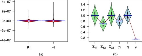
To demonstrate the accuracy of the proposed ECM algorithm, we simulate n = 1000 bivariate skewed VG samples with parameters (31) $\mathit{\mu }=\left(\begin{array}{c}0\\ 0\end{array}\right),\mathbf{\Sigma }=\left(\begin{array}{cc}1& 0.7\\ 0.7& 1\end{array}\right),\mathit{\gamma }=\left(\begin{array}{c}0.8\\ 1\end{array}\right),\mathrm{a}\mathrm{n}\mathrm{d}\nu =0.15$(31) and estimate the parameters using the algorithm specified in Section 4.3. We replicate this experiment r = 1000 times and present the results in Figure 3. Figure 3 shows the violin plots implemented using the caroline package [22] in R which represents the density estimate of the parameter estimates using normal kernel. The median of the estimates are very close to the true parameters of the model implying that the algorithm gives us consistent estimates for these parameters, even when $\nu <\frac{d}{2}$ leading to unbounded density. We also see the distribution of each component of the parameters in $\mathbf{\Sigma }$, $\mathit{\gamma }$, and ν appear to follow roughly a normal distribution. On the other hand, the distribution of $\mathit{\mu }$ has high density around $\mathbf{0}$ and extreme heavy-tails.

Figure 3. Vioplots to show accuracy of parameter estimates for VG distribution in the first simulation study. The median is displayed as a grey box which is connected by a crimson line. True parameter values represented by the blue lines is drawn for comparison. (a) Vioplot of $\mathit{\mu }$ and (b) Vioplot of $\mathbf{\Sigma }$, $\mathit{\gamma }$, ν.

To illustrate the idea of the local point search and line-search in Sections 4.2.2 and 4.2.4 graphically, readers may refer to Figure 2 of Ref. [11]. The figure shows that a global maximum lies roughly between data points along the cusp lines. These cusp lines make computation more demanding as we cannot purely rely on derivative-based methods (see Equation (23(23) $\begin{array}{rl}\frac{\mathrm{\partial }}{\mathrm{\partial }\mathit{\mu }}{\ell }_{\mathrm{N}}^{\mathrm{L}\mathrm{O}\mathrm{O}}& \approx -\frac{1}{2}\left(\frac{\mathrm{\partial }}{\mathrm{\partial }\mathit{\mu }}\sum _{t\ne \kappa \left({\mathit{\mu }}^{\left(k\right)}\right)}\widehat{1/u_t}\right({\mathit{y}}_t-\mathit{\mu }-u_t\mathit{\gamma }{)}^{\mathrm{\top }}{\mathbf{\Sigma }}^{-1}({\mathit{y}}_t-\mathit{\mu }-u_t\mathit{\gamma }))\\ & ={\mathbf{\Sigma }}^{-1}\sum _{t\ne \kappa \left({\mathit{\mu }}^{\left(k\right)}\right)}\widehat{1/u_t}({\mathit{y}}_t-\mathit{\mu }-u_t\mathit{\gamma }).\end{array}$(23) )). The local point search and then the line search serves as an efficient iterative method to obtain estimates which will converge towards the global maximum approximately. To explain the idea, the local point search takes the estimates $\hat{\mathit{\mu }}$ along the black solid line to one of the three data points (red circles) closer to the global maximum point (yellow triangle), while the CM-step and line search improves $\hat{\mathit{\mu }}$ along the black dash line to the point in blue square so that they converge closer towards the global maximum point which lies on the cusp line between two of the data points.

5.2. Comparison of WLOO, LOO and full likelihood methods

We assess the performance of WLOO, LOO likelihood relative to other full likelihood methods including the R package called ghyp in a simulation study. Nitithumbundit and Chan [6] proposed an ECM algorithm [7] to estimate parameters for the VG distribution with unbounded density by capping the density within a small interval of the location parameter. Specifically, they bounded the conditional expectations of (19(19) $\begin{array}{rl}\mathbb{E}(u_t|\mathit{y},\mathit{\theta })& \sim \{\begin{array}{ll}\frac{2\nu -d}{2\nu +{\mathit{\gamma }}^{\mathrm{\top }}{\mathbf{\Sigma }}^{-1}\mathit{\gamma }}& \mathrm{i}\mathrm{f}\nu >\frac{d}{2},\\ -\frac{1}{(2\nu +{\mathit{\gamma }}^{\mathrm{\top }}{\mathbf{\Sigma }}^{-1}\mathit{\gamma })\log \left(z_t\right)}& \mathrm{i}\mathrm{f}\nu =\frac{d}{2},\\ \frac{\mathrm{\Gamma }(\nu -\frac{d}{2}+1)}{\mathrm{\Gamma }(\frac{d}{2}-\nu )}{2}^{2\nu -d+1}(2\nu +{\mathit{\gamma }}^{\mathrm{\top }}{\mathbf{\Sigma }}^{-1}\mathit{\gamma }{)}^{\frac{d}{2}-\nu -1}{z}_t^{d-2\nu }& \mathrm{i}\mathrm{f}\nu \in (\frac{d}{2}-1,\frac{d}{2}),\\ -\log \left(z_t\right)z_t^2& \mathrm{i}\mathrm{f}\nu =\frac{d}{2}-1,\\ \frac{z_t^2}{d-2(\nu +1)}& \mathrm{i}\mathrm{f}\nu <\frac{d}{2}-1,\end{array}\end{array}$(19) ) to (21(21) $\begin{array}{rl}\mathbb{E}(\log u_t|\mathit{y},\mathit{\theta })& \sim \{\begin{array}{ll}\psi (\nu -\frac{d}{2})-\log \left(\frac{2\nu +{\mathit{\gamma }}^{\mathrm{\top }}{\mathbf{\Sigma }}^{-1}\mathit{\gamma }}{2}\right)& \mathrm{i}\mathrm{f}\nu >\frac{d}{2},\\ \log z_t& \mathrm{i}\mathrm{f}\nu =\frac{d}{2},\\ 2\log z_t& \mathrm{i}\mathrm{f}\nu <\frac{d}{2}.\end{array}\end{array}$(21) ) around $\mathit{\mu }$ by a region such that if $z_t<\mathrm{\Delta }$ where Δ is some small fixed positive capping level and $z_t$ is defined in Equation (18(18) $\begin{array}{rl}{K}_{\lambda }^{(1,0)}\left(z\right)& \approx \frac{K_{\lambda +h}\left(z\right)-K_{\lambda -h}\left(z\right)}{2h},\\ z_t^2& =({\mathit{y}}_t-\mathit{\mu }{)}^{\mathrm{\top }}{\mathbf{\Sigma }}^{-1}({\mathit{y}}_t-\mathit{\mu }),\end{array}$(18) ), then the conditional expectations are calculated by replacing $z_t$ with $z_t^{\ast }=max(z_t,\mathrm{\Delta })$. To improve the rate of convergence, they further considered a data augmentation algorithm called the alternating ECM (AECM) by setting $u_t^{\left(k\right)}=w_t/a\left({\mathit{\theta }}^{\left(k\right)}\right)$ where the positive function $a\left(\mathit{\theta }\right)=\xi$ and updated ξ by choosing $\hat{\xi }=\underset{\xi >0}{\mathrm{a}\mathrm{r}\mathrm{g}\mathrm{m}\mathrm{a}\mathrm{x}}{\ell }_{VG}(\hat{\mathit{\mu }},\frac{\hat{\mathbf{\Sigma }}}{\xi },\frac{\mathit{\gamma }}{\xi },\hat{\nu })$using numerical optimisation techniques given the current estimates $(\hat{\mathit{\mu }},\hat{\mathbf{\Sigma }},\mathit{\gamma },\hat{\nu })$. Then they updated the parameters as ${\hat{\mathit{\gamma }}}^{\ast }=\frac{\hat{\mathit{\gamma }}}{\hat{\xi }}$ and ${\hat{\mathbf{\Sigma }}}^{\ast }=\frac{\hat{\mathbf{\Sigma }}}{\hat{\xi }}$. Lastly, they showed that the optimal Δ decreases as ν decreases. Hence they proposed an adaptive Δ method by updating ${\mathrm{\Delta }}^{(k+1)}=\hat{g}({\nu }^{(k+1)},d)$ where $g(\nu ,d)$ is a cubic spline by fitting the median (over repeats) of the optimal Δ across ν and d in a simulation study. The following likelihood methods are considered in this study:

1. Full likelihood ghyp package: ECM algorithm with Δ set to $\mathtt{\text{.Machine\$double.}}\mathtt{e}\mathtt{p}\mathtt{s}\mathtt{0.25}$ $\approx \mathtt{1.2}\mathtt{e}\mathtt{-}\mathtt{4}$ which is a tolerance level of many R functions.

2. Full likelihood fixed Δ : AECM algorithm with the smallest $\mathrm{\Delta }=$

   $\mathtt{\text{sqrt(.Machine\$double.xmin)}}\approx \mathtt{\text{1.5e-154}}$ to provide numerical stability where double.xmin represents the smallest non-zero normalised floating-point number in R.

3. Full likelihood adaptive Δ: AECM algorithm with adaptive Δ.

4. LOO likelihood: ECME/AECM algorithm with LPS (Section 4.2.2), line search (Section 4.2.4) and the smallest Δ which is relevant when there is data multiplicity.

5. WLOO likelihood: ECM algorithm with LPS and line search.

Details of these five likelihood methods are summarised in Table 1.

Table 1. ghyp, fixed Δ, adaptive Δ, LOO and WLOO likelihood methods.

Likelihood method	ECM algorithm	Δ
Full ghyp	MCECM	1.2e-4
Full fixed Δ	AECM	1.5e-154
Full adaptive Δ	AECM	adaptive
LOO	ECM/AECM with LPS & line search	1.5e-154
WLOO	ECM with LPS & line search	–

To conduct the simulation study, we create data multiplicity in two ways: replicate each data point R times or round each data point to D decimal places. The procedure for the simulation study are summarised below:

Step 1:	Choose $\nu =0.05,0.1,\dots ,1.45,1.5$ and $R=1,\dots ,5$ or $D=\mathrm{\infty },8,6,5,4$ for Section 5.2.2. The density is unbounded if $\nu <1$ and cusped if $1\le \nu \le 1.5$ for dimension d = 2.
Step 2:	Simulate n = 1000 data from the bivariate VG distribution with true parameters $\mathit{\mu }$, $\mathbf{\Sigma }$ and $\mathit{\gamma }$ given in (31(31) $\mathit{\mu }=\left(\begin{array}{c}0\\ 0\end{array}\right),\mathbf{\Sigma }=\left(\begin{array}{cc}1& 0.7\\ 0.7& 1\end{array}\right),\mathit{\gamma }=\left(\begin{array}{c}0.8\\ 1\end{array}\right),\mathrm{a}\mathrm{n}\mathrm{d}\nu =0.15$(31) ) and the chosen ν. Then repeat each data point R times, or round each data point to D decimal places.
Step 3:	Apply the five likelihood methods in Table 1 to the data sets to obtain five sets of estimates.
Step 4:	Repeat these steps until we have r = 500 replicates for each method, level of ν, and level of R or D.

5.2.1. No data multiplicity

The median of the measures of accuracy for the four parameters are reported in Table 2. Results show that full likelihood methods using ghyp and fixed Δ mostly give the largest biases whereas adaptive Δ full likelihood, LOO likelihood and WLOO likelihood methods perform similarly with lower biases particularly for $\mathit{\mu }$ when the density is unbounded. It is reasonable to see that LOO and WLOO likelihood methods give very similar results for data without data multiplicity. As ν decreases, the bias seems to increase for $|\hat{\mathbf{\Sigma }}|$ and decrease for $\hat{\mathit{\mu }}$ but there is no clear trend for $\hat{\mathit{\gamma }}$.

Table 2. Median of 500 accuracy measures of parameter estimates across five likelihood methods with no data multiplicity (R = 1). ‘*’ indicates the methods with lowest absolute error.

Measures	Methods	$\nu =0.05$	$\nu =0.1$	$\nu =0.2$	$\nu =0.5$	$\nu =0.75$	$\nu =1$	$\nu =1.5$
$|\hat{\mathit{\mu }}-\mathit{\mu }|$	Full ghyp	1.2e-10	9.3e-10	7.7e-7	0.0067	0.020	0.031	0.050
	Full fixed Δ	3.5e-28	7.1e-14	6.8e-7	0.0054	0.017	0.030	0.049*
	Full adaptive Δ	3.8e-28	7.7e-14	6.8e-7	0.0036	0.012*	0.026*	0.049*
	LOO	1.6e-28*	1.5e-14*	1.1e-7*	0.0014*	0.012*	0.027	0.050
	WLOO	1.6e-28*	1.5e-14*	1.1e-7*	0.0014*	0.012*	0.027	0.050
$\log \left|\hat{\mathbf{\Sigma }}\right|-\log \left|\mathbf{\Sigma }\right|$	Full ghyp	−3.943	−0.601	−0.038*	−0.016*	0.009*	0.023	−0.013
	Full fixed Δ	−0.103*	0.010*	0.117	0.339	0.472	0.549	−0.012
	Full adaptive Δ	−0.143	−0.059	−0.048	−0.027	−0.010	−0.007	−0.012
	LOO	−0.231	−0.126	−0.074	−0.026	−0.015	−0.009*	−0.011*
	WLOO	−0.232	−0.126	−0.074	−0.026	−0.015	−0.009*	−0.011*
$|\hat{\mathit{\gamma }}-\mathit{\gamma }|$	Full ghyp	0.243	0.060	0.038*	0.038	0.043	0.048	0.059*
	Full fixed Δ	0.048*	0.043	0.038*	0.037	0.039	0.048	0.059*
	Full adaptive Δ	0.048*	0.042*	0.039	0.037	0.038	0.045*	0.059*
	LOO	0.061	0.050	0.041	0.036*	0.038*	0.045*	0.059*
	WLOO	0.061	0.050	0.041	0.036*	0.038*	0.045*	0.059*
$\log \hat{\nu }-\log \nu$	Full ghyp	0.1376	0.0368	0.0067*	−0.0047*	−0.0418	−0.0809	0.0033
	Full fixed Δ	−0.0259	−0.0667	−0.1571	−0.4636	−0.7097	−0.9199	0.0022*
	Full adaptive Δ	0.0052*	0.0055*	0.0091	0.0103	0.0024*	0.0010*	0.0033
	LOO	0.0092	0.0093	0.0110	0.0123	0.0142	0.0090	0.0167
	WLOO	0.0092	0.0093	0.0110	0.0123	0.0142	0.0090	0.0167

5.2.2. Data multiplicity due to repetition and rounding

To visualise the differences in performance better, we transform the accuracy measures by $-\log [\log (-\log |\hat{\mathit{\mu }}-\mathit{\mu }|\left)\right]$, $\log |\log |\hat{\mathbf{\Sigma }}|-\log |\mathbf{\Sigma }||$, $\log |\hat{\mathit{\gamma }}-\mathit{\gamma }|$ and $\log |\log \hat{\nu }-\log \nu |$ respectively and graph the transformed accuracy measures in Figure 4 for replicated data when R = 1, 3, 5. Since the plot for rounded data is very similar, it is omitted. See Ref. [23], page 95 for this plot. We remark that the transformation $f\left(x\right)=-\log [\log (-\log x\left)\right]$ for $|\hat{\mathit{\mu }}-\mathit{\mu }|$ is monotonically increasing on $(0,1/e)$.

Figure 4. Plot of transformed accuracy measures for full ghyp package (red solid line), full fixed Δ (light green striped line), full adaptive Δ (dotted green line), LOO (blue dot & striped line), and WLOO (dash magenta line) likelihoods. The columns from left to right represents the median parameter accuracy measures for $(\hat{\mathit{\mu }},\hat{\mathbf{\Sigma }},\hat{\mathit{\gamma }},\hat{\nu })$ respectively. The rows from top to bottom represents R = 1, 3, 5 respectively where R is the number of times each data point is repeated.

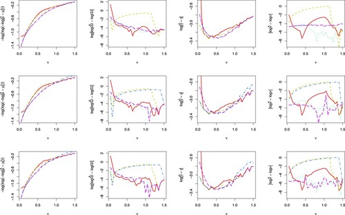
With data repetition, the WLOO likelihood (magenta line) generally performs better than other likelihood methods for all levels of ν in Figure 4. The full likelihood ghyp with ${\mathrm{\Delta }}_0=$ 1.2e-4 (red line) and adaptive Δ (green line) methods provide reasonable accuracy when $\nu >0.15$ but the adaptive Δ method is better and similar to WLOO for $\hat{\nu }$. This result is in agreement with the optimal Δ choice study in Section 4.2 of Ref. [6]. They considered ${\mathrm{\Delta }}_1=$ 1.49e-154 and ${\mathrm{\Delta }}_2=$ 1.49e-8 and plotted in Figure 2, the log of the sum of mean absolute errors (MAE) over all the parameters for a $d=2$ dimensional VG model with $\mathit{\mu }=\mathbf{0}$, $\mathbf{\Sigma }=\left[\begin{array}{cc}1& -04\\ -0.4& 1\end{array}\right]$ and $\mathit{\gamma }=(-1.2,-0.2)$ using the AECM algorithm. Results show that ${\mathrm{\Delta }}_1$ performs better for much smaller shape parameter at $\nu <0.15$ whereas ${\mathrm{\Delta }}_2$ performs better for $0.15<\nu <1.15$ approximately. Since ${\mathrm{\Delta }}_0$ is similar to ${\mathrm{\Delta }}_2$ relative to ${\mathrm{\Delta }}_1$, this result explains why full and LOO likelihoods both with ${\mathrm{\Delta }}_1$ perform worst in Figure 4 for $0.15<\nu <1.5$ approximately.

When ν is small, full likelihood ghyp method performs poorly as expected. The fixed Δ full and LOO likelihood methods (light green and blue lines) have the worst performance particularly for $\hat{\mathbf{\Sigma }}$ and $\hat{\nu }$ since they both adopt a fixed capping level Δ. The only difference is that the LOO likelihood leaves out a data point while the full likelihood does not. Nevertheless, as the data multiplicity increases, leaving a data point out becomes insignificant and so the accuracies of the full fixed Δ and LOO likelihood converge. As ν approaches 1.5, the accuracy for $\hat{\mathbf{\Sigma }}$ and $\hat{\nu }$ for all likelihood method converges.

With data rounding, the results are very similar. The WLOO likelihood is still better for most cases, such as $\hat{\mathit{\mu }}$ and $\hat{\mathit{\gamma }}$ when $\nu >0.3$ approximately. For $\hat{\nu }$, the full likelihood ghyp package performs well around $0.2<\nu <0.5$, the full adaptive Δ likelihood performs well in the mid-range at around $0.6<\nu <1.2$ and the full fixed Δ likelihood performs well at around $\nu =1.4$. Again, the ghyp package and adaptive Δ full likelihood perform similarly. For $\hat{\mathbf{\Sigma }}$ and $\hat{\nu }$, the full fixed Δ likelihood still performs worse whereas the LOO likelihood is now much better and is similar to WLOO when $\nu >0.3$ but they perform similarly for smaller ν. We remark that for larger ν, the data rounding is insignificant because of the lower peak and hence less data multiplicity around $\hat{\mathit{\mu }}$.

In summary, for both data repetition and rounding cases, we have demonstrated that the full ghyp and fixed Δ likelihood methods using fixed capping levels perform worse and can be improved by providing an adaptive capping level. Moreover, the LOO likelihood method can be extended to the WLOO likelihood to deal with the unbounded likelihood due to data multiplicity. Overall, the WLOO likelihood gives the most stable and accurate results. As the range of ν is uncertain in practice, it is better to use the WLOO likelihood which provides the best overall performance.

5.3. Asymptotic properties for the location parameter of VG distribution

Podgórski and Wallin [5] proved the consistency and super-efficiency of the location parameter estimate using the maximum LOO likelihood as stated in Theorem 3.1 in Section 3.2. They also stated the upper bound for the index of the rate of convergence $\text{β}<1/(1+\alpha )=1/\left(2\nu \right)$ where $\alpha =2\nu -1$ for unbounded univariate VG distribution. The aim of this section is to determine these optimal rates through simulation studies and to analyse the asymptotic distribution of the location parameter estimate for unbounded and cusp densities. In this study, we consider LOO instead of WLOO loglikelihood to investigate the optimal convergence rate of Ref. [5].

We consider univariate case ($d=1$) and set up the simulation as below for $\nu \in (0,1]$:

1. Set the sample size n to be one of the 41 sample sizes $\{500,1000,\dots ,19,500,20,000\}\cup \{100,000\}$.

2. For each sample size, set the true shape parameter ν to be one of the 50 shape parameters $\{0.02,0.04\dots ,0.98,1\}$.

3. For each pair of $(n,\nu )$, generate $r=20,000$ different sets of samples, each set from standard univariate symmetric VG distribution with shape parameter ν and sample size n.

4. For the ith set of 20,000 samples, estimate ${\hat{\mu }}_{n,\nu ,i}$ by searching through each mid data points and choosing the one that maximises the LOO log-likelihood where the other parameters $({\sigma }^2=1,\gamma =0,\nu )$ are fixed.

This gives us for each pair of $(n,\nu )$ the sample ${\hat{\mu }}_{n,\nu ,1:20,000}$ of $r=20,000$ estimates which is used to study the optimal convergence rate and asymptotic distribution across sample size n and shape parameter ν.

5.3.1. Optimal convergence rate

Since the scale of asymptotic distribution of ${\hat{\mu }}_{n,\nu ,1:20,000}$ changes with n according to the convergence rate $n^{-{\text{β}}_{\nu }}$, we can fit a power curve to estimate ${\text{β}}_{\nu }$ in the optimal convergence rate. We choose a robust measure of spread called the median absolute deviation ($\mathrm{M}\mathrm{A}\mathrm{D}$) from 0 defined by ${\mathrm{M}\mathrm{A}\mathrm{D}}_{n,\nu }\stackrel{△}{=}\mathrm{m}\mathrm{e}\mathrm{d}\mathrm{i}\mathrm{a}\mathrm{n}(|{\mu }_{n,\nu ,1}|,\dots ,|{\mu }_{n,\nu ,20,000}|).$For each ν, we fit a power curve to the ${\mathrm{M}\mathrm{A}\mathrm{D}}_{n,\nu }$ against n. In other words, we find parameters $a_{\nu }$ and $b_{\nu }$ such that ${\mathrm{M}\mathrm{A}\mathrm{D}}_{n,\nu }=a_{\nu }{n}^{b_{\nu }}$. This is equivalent to fitting a simple linear regression model $\log {\mathrm{M}\mathrm{A}\mathrm{D}}_{n,\nu }=\log a_{\nu }+b_{\nu }\log n$ to obtain the estimates $({\widehat{\log a}}_{\nu },{\hat{b}}_{\nu })$. Then an estimate of the optimal rate for a given ν is obtained by setting ${\widehat{\text{β}}}_{\nu }=-{\hat{b}}_{\nu }$. We repeat this process for the other ν's.

Figure 5(a) plots the relative error of ${\widehat{\text{β}}}_{\nu }$ against ν along with its confidence intervals. From the figure, ${\widehat{\text{β}}}_{\nu }$ appears to follow the proposed optimal rate of $1/\left(2\nu \right)$ when $0<\nu \le 0.4$. However when $0.4<\nu <1$ (the density is bounded with a cusp when $0.5<\nu <1$), ${\widehat{\text{β}}}_{\nu }$ appears to be slightly different and the relative error follows a sinusoidal pattern. In fact for $0.4<\nu <0.76$, ${\widehat{\text{β}}}_{\nu }$ appears to be greater than the proposed optimal convergence rate index. For $0.76<\nu <1$, ${\widehat{\text{β}}}_{\nu }$ appears to be less than the proposed optimal convergence rate index. As ν approaches to 1, ${\widehat{\text{β}}}_{\nu }$ approaches the convergence rate for asymptotic normality. Overall the estimated optimal rate is consistent with Theorem 3.1 in Section 3.2 in the range of $\nu <0.5$ for unbounded density. As for $0.5\le \nu \le 1$, more theoretical studies is needed to understand the behaviour of the location parameter estimates ${\hat{\mu }}_{n,\nu ,1:20,000}$. To investigate this unusual behaviour of ${\hat{\mu }}_{n,\nu ,1:20,000}$, we further analyse the asymptotic distribution of ${\hat{\mu }}_{n,\nu ,1:20,000}$ across ν when $n=100,000$ is large.

Figure 5. (a) Relative error $\frac{{\widehat{\text{β}}}_{\nu }-{\text{β}}_{\nu }}{{\text{β}}_{\nu }}$ (solid black) against ν. The horizontal solid grey line indicates agreement of ${\widehat{\text{β}}}_{\nu }$ with the proposed optimal rate ${\text{β}}_{\nu }=\frac{1}{2\nu }$. The vertical grey dotted lines represent grid lines for $\nu =\{0,0.2,0.4,0.6,0.8,1\}$. We also include the 95% confidence interval for the relative error (dashed grey). (b) Density of estimates ${\hat{\mu }}_{n,\nu ,1:20,000}$ with its scale standardised using $\mathrm{M}\mathrm{A}\mathrm{D}$ for each ν where n = 100, 000. We use a rainbow colour scheme ranging from red ($\nu =0.02$) to magenta ($\nu =1$).

5.3.2. Asymptotic distribution

This section explores the distribution of ${\hat{\mu }}_{n,\nu ,1:20,000}$ or $\log |{\hat{\mu }}_{n,\nu ,1:20,000}|$ in the more appropriate scale and approximate the distribution to allow SE calculation for $\hat{\mu }$.

Analysis 1: preview the distribution of location parameter estimates using normal kernel

We begin with plotting the normal kernel density estimate in Figure 5(b) for ${\hat{\mu }}_{n,\nu ,1:20,000}$ with its scale standardised using $\mathrm{M}\mathrm{A}\mathrm{D}$, taking $n=100,000$ and representing the density for each ν in rainbow colours. We note that the estimated density exhibits heavier tails and sharper peaks at the expense of intermediate tails as ν decreases (from magenta line to red line) and this feature resembles VG distribution.

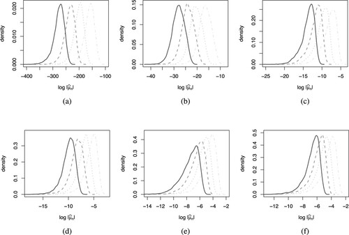
Analysis 2: explore the distribution on the more appropriate log scale

To explore the distributions on a more appropriate scale, we transform ${\hat{\mu }}_{n,\nu ,1:20,000}$ to $\log |{\hat{\mu }}_{n,\nu ,1:20,000}|$ and plot the kernel density estimates in Figure 6 for $(n,\nu )=(1000,5000,20,000,100,000)$ by $(0.02,0.2,$ $0.4,0.6,0.8,1)$. We observe that the location of the distribution shifts to the right in general for each ν as the sample size n increases but the scale and the shape of the distribution remain relatively similar. An exception is when $\nu =0.8$ where the scale gets slightly larger and the shape becomes less left skewed. We remark that these densities resemble the densities of the generalised Gumbel (GG) distribution. Fitting the GG distribution to $\log |{\hat{\mu }}_{n,\nu ,1:20,000}|$ corresponds to fitting a double generalised gamma (DGG) distribution to ${\hat{\mu }}_{n,\nu ,1:20,000}$. See Appendices A and B for details of the two distributions, respectively.

Figure 6. Kernel density estimates of $\log |{\hat{\mu }}_n|$'s for $\nu =0.02,0.2,0.4,0.6,0.8,1$ and n = 1000 (solid black), 5000 (dashed dark grey), 20, 000 (dotted grey), 100, 000 (dash-dotted light grey) with each n being combined into a single plot for comparison. (a) density plots for $\nu =0.02$ (b) density plots for $\nu =0.2$ (c) density plots for $\nu =0.4$ (d) density plots for $\nu =0.6$ (e) density plots for $\nu =0.8$ and (f) density plots for $\nu =1$.

Analysis 3: approximate the distribution on the log scale

This analysis aims to approximate the kernel densities for $\log |{\hat{\mu }}_{n,\nu ,1:20,000}|$ in Figure 6 with some distributions which should include log-normal as the asymptotic distribution when ν approaches or exceeds 1. In the search for these distributions, we start with VG based on Figure 5(b) and check the goodness-of-fit using P-P plots by plotting the cumulative distribution function (cdf) $F(\log |{\hat{\mu }}_{n,\nu ,1:20,000}|;{\mathit{\theta }}_{\nu })$ against the ordered sequence $(1:20,000)/20,001$ giving one P-P plot for each $\nu =0.02,0.04,\dots ,1$ and taking n = 100, 000. We also consider stable distribution which, like normal, can model any properly normed sums of independent and identically distributed random variables. If each variable has a finite variance, classical central limit theorem states that the sum will tend toward a normal distribution as the number of variables increases but without the finite variance assumption, the limit may be a stable distribution. These provide some theoretical ground for the trial although it still does not address the unbounded density problem. However, the P-P plots for both log-VG and log-stable distributions argue against adoption. Finally, we try DGG distribution with the flexible generalised gamma distribution on each side and the cdf of GG distribution for fitting $\log |{\hat{\mu }}_{n,\nu ,1:20,000}|$ is given by Equation (A2(A2) $F_{\mathrm{G}\mathrm{G}}\left(x\right)=F_{\mathrm{g}\mathrm{a}\mathrm{m}\mathrm{m}\mathrm{a}}(\exp (\mu +\sigma x);m,m),x>0$(A2) ) evaluated at the fitted parameters ${\hat{\mathit{\theta }}}_{\nu }=({\hat{\mu }}_{\mathrm{G}\mathrm{G}},{\hat{\sigma }}_{\mathrm{G}\mathrm{G}},{\hat{m}}_{\mathrm{G}\mathrm{G}})$. As the set of P-P plots for GG distribution shows near-perfect straight lines except some very minimal deviations around the 25th and 75th percentiles for $0.22\le \nu \le 0.34$, we confirm that GG distribution fits $\log |{\hat{\mu }}_{n,\nu ,1:20,000}|$ the best amongst the log-VG and log-stable distributions. See Ref. [23], pages 77-78 for these P-P plots. Hence we choose DGG to approximate the distribution for the location parameter estimate μ using maximum LOO likelihood. We declare the limitation of this ad hoc search but based on the P-P plots, we are confident that DGG distribution can provide a reasonably accurate standard error (SE) estimate for $\hat{\mu }$. We will demonstrate the calculation and confirm the accuracy.

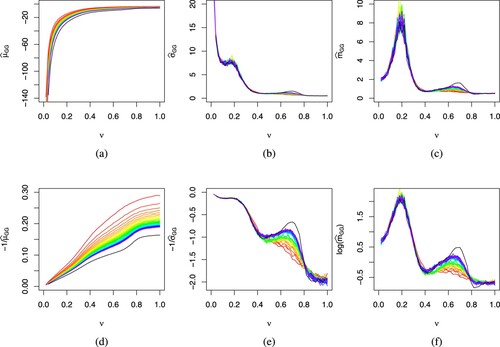
Analysis 4: assess the convergence of DGG distribution to asymptotic distribution

We assess the convergence of DGG distribution as n increases to asymptotic distribution by plotting in Figure 7 the parameter estimates $({\hat{\mu }}_{\mathrm{G}\mathrm{G}},{\hat{\sigma }}_{\mathrm{G}\mathrm{G}},{\hat{m}}_{\mathrm{G}\mathrm{G}})$ against ν when fitting the $\log |{\hat{\mu }}_{n,\nu ,1:20,000}|$ for each $(n,\nu )$ to GG distribution while different n is represented by lines in rainbow colours from red for the lowest n = 500. We also plot the transformed parameter estimates to view the behaviour across ν more clearly. As ν decreases, ${\hat{\mu }}_{\mathrm{G}\mathrm{G}}$ in Figure 7(a,d) appears to drop roughly at a hyperbolic rate with some minor curvature for larger values of ν. This agrees with the observation in Figure 6 that the location of the density shifts to the left as ν decreases. However, ${\hat{\sigma }}_{\mathrm{G}\mathrm{G}}$ in Figure 7(b,c) increases at a hyperbolic rate with two bumps as ν decreases. This increase in the spread can also be observed in the densities of Figure 6. The two bumps occur around $\nu =0.2$ and $\nu =0.7$ with the left one showing more fluctuation and no clear distinction between each n possibly due to sampling error whereas the right one has a clear distinction between each n especially for n = 100, 000. In Figure 7(c,f), ${\hat{m}}_{\mathrm{G}\mathrm{G}}$ also has two bumps similar to ${\hat{\sigma }}_{\mathrm{G}\mathrm{G}}$ but unlike ${\hat{\mu }}_{\mathrm{G}\mathrm{G}}$ and ${\hat{\sigma }}_{\mathrm{G}\mathrm{G}}$, ${\hat{m}}_{\mathrm{G}\mathrm{G}}$ tends to some constant value as ν approaches to 0. The right bumps for both ${\hat{\sigma }}_{\mathrm{G}\mathrm{G}}$ and ${\hat{m}}_{\mathrm{G}\mathrm{G}}$ suggest that the DGG distribution for $\hat{\mu }$ has yet to converge to the asymptotic distribution and it is unclear how large n should be for the convergence for $0.5\le \nu \le 1$, the range with cusp density. Adding to the inconsistency of the index for optimal convergence rate as displayed in Figure 5, the asymptotic properties for this range of ν worth further analyses.

Figure 7. Plot of estimates of generalized Gumbel distribution fitted to the distribution of $\log |{\hat{\mu }}_n|$ against ν. Row 1 plots the $({\hat{\mu }}_{\mathrm{G}\mathrm{G}},{\hat{\sigma }}_{\mathrm{G}\mathrm{G}},{\hat{m}}_{\mathrm{G}\mathrm{G}})$ against ν, respectively, while row 2 plots the transformation $(1/{\hat{\mu }}_{\mathrm{G}\mathrm{G}},-1/{\hat{\sigma }}_{\mathrm{G}\mathrm{G}},\log {\hat{m}}_{\mathrm{G}\mathrm{G}})$ against ν, respectively, to enlarge certain portion of the plots. A rainbow colour scheme ranging from red (n = 500) to magenta (n = 20, 000) is used to denote sample size and the black line represents n = 100, 000. (a) ${\hat{\mu }}_{\mathrm{G}\mathrm{G}}$ vs ν (b) ${\hat{\sigma }}_{\mathrm{G}\mathrm{G}}$ vs ν (c) ${\hat{m}}_{\mathrm{G}\mathrm{G}}$ vs ν (d) $-1/{\hat{\mu }}_{\mathrm{G}\mathrm{G}}$ vs ν (e) $-1/{\hat{\sigma }}_{\mathrm{G}\mathrm{G}}$ vs ν and (f) $\log {\hat{m}}_{\mathrm{G}\mathrm{G}}$ vs ν.

Demonstration of SE calculation for the location parameter estimate using DGG distribution

Lastly, we demonstrate the SE calculation for $\hat{\mathit{\mu }}$ (d = 2) using DGG distribution and the true parameters in Section 5.1 as the sample estimates. For each component ${\hat{\mathit{\mu }}}_j$, we apply the GG distribution to estimate the variability of $\log |{\hat{\mathit{\mu }}}_j|$. Specifically, we use $\hat{\nu }=0.15$ with sample size n = 1000 to extrapolate the values $-1/{\hat{\mu }}_{\mathrm{G}\mathrm{G}}=0.0466,-1/{\hat{\sigma }}_{\mathrm{G}\mathrm{G}}=-0.1291$ and $\log {\hat{m}}_{\mathrm{G}\mathrm{G}}=1.8733$ by applying the spline function in R to Figure 7(d–f). This gives the GG parameter estimates ${\hat{\mu }}_{\mathrm{G}\mathrm{G}}=-21.4431,{\hat{\sigma }}_{\mathrm{G}\mathrm{G}}=7.7431$ and ${\hat{m}}_{\mathrm{G}\mathrm{G}}=6.5098$. Applying these estimates to Equation (A5(A5) $\mathrm{M}\mathrm{A}\mathrm{D}\left({\hat{\mathit{\mu }}}_i\right)\approx Q_{\mathrm{g}\mathrm{e}\mathrm{n}\mathrm{g}\mathrm{a}\mathrm{m}\mathrm{m}\mathrm{a}}\left(0.5\right)=\sqrt{{\hat{\mathrm{\Sigma }}}_{ii}}{Q}_{\mathrm{g}\mathrm{a}\mathrm{m}\mathrm{m}\mathrm{a}}{(0.5;m_{\mathrm{G}\mathrm{G}},m_{\mathrm{G}\mathrm{G}}\exp (-{\mu }_{\mathrm{G}\mathrm{G}}/{\sigma }_{\mathrm{G}\mathrm{G}}\left)\right)}^{{\sigma }_{\mathrm{G}\mathrm{G}}}$(A5) ) with ${\hat{\mathrm{\Sigma }}}_{11}=1$ and ${\hat{\mathrm{\Sigma }}}_{22}=1$ gives us the MADs $\begin{array}{r}\hat{\mathrm{M}}{\mathrm{A}\mathrm{D}}_{n,\nu }\left(\hat{\mathit{\mu }}\right)=\left(\begin{array}{c}\mathrm{M}\mathrm{A}\mathrm{D}\left({\hat{\mu }}_1\right)\\ \mathrm{M}\mathrm{A}\mathrm{D}\left({\hat{\mu }}_2\right)\end{array}\right)\approx \left(\begin{array}{c}3.25\times {10}^{-10}\\ 3.25\times {10}^{-10}\end{array}\right)\end{array}$using DGG distribution which are close to the ‘observed’ MAD${}_{n,\nu }$ $\begin{array}{r}{\mathrm{M}\mathrm{A}\mathrm{D}}_{n,\nu }\left(\hat{\mathit{\mu }}\right)=\left(\begin{array}{c}3.16\times {10}^{-10}\\ 2.85\times {10}^{-10}\end{array}\right)\end{array}$by applying ${\mathrm{M}\mathrm{A}\mathrm{D}}_{n,\nu }\left(\mathit{x}\right)=\mathrm{m}\mathrm{e}\mathrm{d}\mathrm{i}\mathrm{a}\mathrm{n}(|\mathit{x}-\mathrm{m}\mathrm{e}\mathrm{d}\mathrm{i}\mathrm{a}\mathrm{n}(\mathit{x}\left)|\right)$ to the simulated sample ${\hat{\mathit{\mu }}}_{j,n,\nu ,1:r}$ with r = 1000 replicates. Hence $\hat{\mathrm{M}}{\mathrm{A}\mathrm{D}}_{n,\nu }$ estimated from DGG distribution provides reasonably accurate estimates of MAD${}_{n,\nu }$, unobserved in practice, for the SE estimate of $\hat{\mathit{\mu }}$ using maximum LOO likelihood when the shape parameter $\nu \in (0,\frac{d}{2})$ gives unbounded density or $\nu \in (\frac{d}{2},\frac{d+1}{2})$ gives cusp density. Using $\hat{\mathrm{M}}{\mathrm{A}\mathrm{D}}_{n,\nu }$ as SE estimate, we can also construct confidence interval for $\hat{\mathit{\mu }}$.

6. Conclusion

Optimising a non-convex likelihood is always challenging particularly for noisy data with cusped or unbounded likelihood. An obvious example is the estimation of $\mathit{\mu }$ from VG distribution when $\nu \le \frac{d}{2}$. We propose ECM algorithm using hierarchical model via the NMVM representation of VG distribution to avoid the direct maximisation of full likelihood. Conditional on the mixing variable $u_t$, ${\mathit{y}}_t$ follows a condition normal distribution in (2(2) $\mathit{y}|u\sim {\mathcal{N}}_d(\mathit{\mu }+\mathit{\gamma }u,u\mathbf{\Sigma }),u\sim \mathcal{G}(\nu ,\nu )$(2) ). In case ${\mathit{y}}_t\to \mathit{\mu }$ and $\nu \le \frac{d}{2}$ when the density becomes unbounded in (3(3) $\begin{array}{r}{f}_{\mathrm{V}\mathrm{G}}\left(\mathit{y}\right)\sim \{\begin{array}{ll}{2}^{\nu -d}{\pi }^{-\frac{d}{2}}{\left|\mathbf{\Sigma }\right|}^{-\frac{1}{2}}\frac{\mathrm{\Gamma }(\nu -\frac{d}{2})}{\mathrm{\Gamma }\left(\nu \right)}\frac{{\nu }^{\nu }}{(2\nu +{\mathit{\gamma }}^{\mathrm{\top }}{\mathbf{\Sigma }}^{-1}\mathit{\gamma }{)}^{\frac{2\nu -d}{2}}}& \mathrm{i}\mathrm{f}\nu >\frac{d}{2},\\ -2^{1-d}{\pi }^{-\frac{d}{2}}{\left|\mathbf{\Sigma }\right|}^{-\frac{1}{2}}\frac{d^{\frac{d}{2}}}{\mathrm{\Gamma }\left(\frac{d}{2}\right)}\log \left(z\right)& \mathrm{i}\mathrm{f}\nu =\frac{d}{2},\\ 2^{-\nu }{\pi }^{-\frac{d}{2}}{\left|\mathbf{\Sigma }\right|}^{-\frac{1}{2}}\frac{\mathrm{\Gamma }(\frac{d}{2}-\nu )}{\mathrm{\Gamma }\left(\nu \right)}{\nu }^{\nu }{z}^{2\nu -d}& \mathrm{i}\mathrm{f}\nu <\frac{d}{2}.\end{array}\end{array}$(3) ), $\mathbb{E}(\frac{1}{u_t}|\mathbf{\text{y}},\mathit{\theta })\to \mathrm{\infty }$ in (17(17) $\begin{array}{rl}\widehat{\log u_t}& =\mathbb{E}(\log u_t|\mathit{y},\mathit{\theta })=\log \left(\frac{z_t}{\sqrt{2\nu +{\mathit{\gamma }}^{\mathrm{\top }}{\mathbf{\Sigma }}^{-1}\mathit{\gamma }}}\right)+\frac{K_{\nu -\frac{d}{2}}^{(1,0)}\left(\sqrt{2\nu +{\mathit{\gamma }}^{\mathrm{\top }}{\mathbf{\Sigma }}^{-1}\mathit{\gamma }}{z}_t\right)}{K_{\nu -\frac{d}{2}}\left(\sqrt{2\nu +{\mathit{\gamma }}^{\mathrm{\top }}{\mathbf{\Sigma }}^{-1}\mathit{\gamma }}{z}_t\right)}\end{array}$(17) ). Nitithumbundit and Chan [6] proposed to cap the density but we propose to use LOO likelihood. In case of data multiplicity, we extend the LOO likelihood to WLOO likelihood.

To improve the estimation efficiency, we propose local mid-point search (one-dimensional case in Section 4.2.1) and local point search (higher dimensional case in Section 4.2.2) for $\hat{\mathit{\mu }}$ as well as the line search (Section 4.2.4). The local point searches ensure the location parameter estimates jump closer towards the maximum. Since the derivatives of LOO likelihood in (23(23) $\begin{array}{rl}\frac{\mathrm{\partial }}{\mathrm{\partial }\mathit{\mu }}{\ell }_{\mathrm{N}}^{\mathrm{L}\mathrm{O}\mathrm{O}}& \approx -\frac{1}{2}\left(\frac{\mathrm{\partial }}{\mathrm{\partial }\mathit{\mu }}\sum _{t\ne \kappa \left({\mathit{\mu }}^{\left(k\right)}\right)}\widehat{1/u_t}\right({\mathit{y}}_t-\mathit{\mu }-u_t\mathit{\gamma }{)}^{\mathrm{\top }}{\mathbf{\Sigma }}^{-1}({\mathit{y}}_t-\mathit{\mu }-u_t\mathit{\gamma }))\\ & ={\mathbf{\Sigma }}^{-1}\sum _{t\ne \kappa \left({\mathit{\mu }}^{\left(k\right)}\right)}\widehat{1/u_t}({\mathit{y}}_t-\mathit{\mu }-u_t\mathit{\gamma }).\end{array}$(23) ) are also approximations, the line search ensures monotonicity along the recurrent updates. The first simulation study confirms the accuracy of the location parameter estimate for the VG distribution even though these search procedures do not necessary guarantee that the path leads to a global maximum.

In the second simulation study, our proposed ECM algorithm using WLOO likelihood is compared to three full likelihood methods, namely, MCECM from the ghyp package, AECM with fixed Δ and AECM with adaptive Δ, and one LOO likelihood method. The comparison is conducted under three scenarios: no data multiplicity, data multiplicity due to repetition and data multiplicity due to rounding. Results show that ECM algorithm using WLOO likelihood performs well in all three scenarios.

Lastly, our third simulation study explores empirically the optimal convergence rate and asymptotic distribution for our proposed location parameter estimate using the maximum LOO likelihood method for symmetric univariate VG data. Results show that the index for optimal convergence rate follows $\frac{1}{2\nu }$ when $0<\nu \le 0.4$. However, when $0.4<\nu <1$, the index appears to be slightly different with a sinusoidal pattern for the relative error. As ν approaches 1, the optimal rate approaches the convergence rate for asymptotic normality. Following the result, we propose to approximate the asymptotic distribution using the DGG distribution when $\nu \in (0,1]$ so that we can calculate SE and construct confidence interval for each component of ${\hat{\mathit{\mu }}}_j$. In summary, the idea of the proposed ECM algorithm can be applied to other distributions in NMVM representation including Students' t and GH distributions with some suitable adjustments in the E-step.

Our method using hierarchical model in NMVM representation is similar in spirit to Bayesian methods which are sometimes treated as a frequentist method when flat priors are adopted so that the solution could be considered ‘equivalent’ to the solution using the classical likelihood method. This proxy likelihood approach can avoid the optimisation of complicated likelihoods. Further, the empirical Bayesian (EB) method offers procedures for statistical inference in which the prior $\pi \left(\theta \right)$ is estimated from the data, ie $\pi \left(\theta |\mathit{y}\right)$ without relying on external input (similar to using flat priors). Hossain, Kozubowski, Podgórski[24] proposed the weighted likelihood estimation for a parameter θ as (32) ${\hat{\theta }}_{\mathrm{E}\mathrm{B}}=\sum _{i=1}^n{w}_i{\hat{\theta }}_i=\frac{\sum _{i=1}^n{\hat{\theta }}_{i}L\left({\hat{\theta }}_i|y_i\right)}{\sum _{i=1}^{n}L\left({\hat{\theta }}_i|y_i\right)}\stackrel{\mathrm{L}\mathrm{M}}{=}\frac{\sum _{i=1}^n{y}_i\prod _{j=1}^{n}h(y_j-y_i)}{\sum _{i=1}^n\prod _{j=1}^{n}h(y_j-y_i)},$(32) where ${\hat{\theta }}_i=\upsilon \left(y_i\right)$ is an estimator of θ using the ML principle and observation $y_i$, and the last term in (32(32) ${\hat{\theta }}_{\mathrm{E}\mathrm{B}}=\sum _{i=1}^n{w}_i{\hat{\theta }}_i=\frac{\sum _{i=1}^n{\hat{\theta }}_{i}L\left({\hat{\theta }}_i|y_i\right)}{\sum _{i=1}^{n}L\left({\hat{\theta }}_i|y_i\right)}\stackrel{\mathrm{L}\mathrm{M}}{=}\frac{\sum _{i=1}^n{y}_i\prod _{j=1}^{n}h(y_j-y_i)}{\sum _{i=1}^n\prod _{j=1}^{n}h(y_j-y_i)},$(32) ) is for the location model (LM) $f\left(y_i|\theta \right)=h(y_i-\theta ),y_i\in \mathbb{R}$ and $h(\cdot )$ is a symmetric and unimodal density. This estimation method has an EB flavour since ${\hat{\theta }}_{\mathrm{E}\mathrm{B}}$ can be viewed as the posterior sample mean of ${\hat{\theta }}_i$ with probability $w_i$ where the data-driven prior distribution is discrete and supported on the same values ${\hat{\theta }}_i$ with equal probability 1/n. They showed that the asymptotic normality and efficiency of Bayes estimator using ordinary prior $\pi \left(\theta \right)$ can be applied to EB estimator using empirical sample prior $\pi \left(\theta |\mathit{y}\right)$. Based on the symmetric gamma (SG) distribution with pdf $f_{\mathrm{S}\mathrm{G}}\left(y|\theta \right)=\frac{|y-\theta {|}^{\alpha -1}\exp (-|y-\theta |)}{2\mathrm{\Gamma }\left(\alpha \right)},y\in \mathbb{R},$which is unbounded when $0<\alpha <1$ ($\alpha =1$ corresponds to symmetric Laplace (SL) distribution), they showed that the location parameter θ in LM has a closed-form expression ${\hat{\theta }}_{\mathrm{E}\mathrm{B}}=\frac{\sum _{i=1}^n{y}_i\exp (-\sum _{j\ne i}|x_j-x_i|)\prod _{j\ne i}|y_j-y_i{|}^{\alpha -1}}{\sum _{i=1}^n\exp (-\sum _{j\ne i}|x_j-x_i|)\prod _{j\ne i}|y_j-y_i{|}^{\alpha -1}}$using (32(32) ${\hat{\theta }}_{\mathrm{E}\mathrm{B}}=\sum _{i=1}^n{w}_i{\hat{\theta }}_i=\frac{\sum _{i=1}^n{\hat{\theta }}_{i}L\left({\hat{\theta }}_i|y_i\right)}{\sum _{i=1}^{n}L\left({\hat{\theta }}_i|y_i\right)}\stackrel{\mathrm{L}\mathrm{M}}{=}\frac{\sum _{i=1}^n{y}_i\prod _{j=1}^{n}h(y_j-y_i)}{\sum _{i=1}^n\prod _{j=1}^{n}h(y_j-y_i)},$(32) ) when the estimator ${\hat{\theta }}_i=\upsilon \left(y_i\right)$ is a LOO estimator such that ${\hat{\theta }}_i$ is calculated using the sample without $y_i$. In a simulation study, they showed that ${\hat{\theta }}_{\mathrm{E}\mathrm{B}}$ performs slightly better than ${\hat{\theta }}_{\mathrm{L}\mathrm{O}\mathrm{O}}=\mathrm{a}\mathrm{r}\mathrm{g}\mathrm{m}\mathrm{a}\mathrm{x}\left\{{\ell }^{\mathrm{L}\mathrm{O}\mathrm{O}}\right(y_i|\mathit{y}),i=1,\dots ,n\}$in Tables 5 and 6 for SG and SL distributions in Ref. [24]. This EB method which provides closed-form solution is attractive. Future studies may derive the EB estimates for VG distribution and compare the performance of EB method with our proposed ECM method using WLOO likelihood in several scenarios.

Moreover, our third simulation study for the optimal convergence rate and asymptotic distribution of the location parameter estimate considers only the univariate symmetric case using LOO likelihood. For future work, we will consider multivariate skewed case using WLOO likelihood. Furthermore, in-depth study should be directed to the case of $0.5\le \nu \le 1$ when the density has cusp density as results show inconsistency of the index for the optimal convergence rate and problem of convergence for the asymptotic distribution. Furthermore, the dependence between the location and other parameters of VG distribution should also be considered in the simulation studies. Lastly, it is worth exploring better approximation to the asymptotic distribution from both numerical and theoretical perspectives even though it can be challenging.

Disclosure statement

No potential conflict of interest was reported by the author(s).

Appendix

A Generalised Gumbel (GG) distribution

The pdf of a GG distribution is given by (A1) $f_{\mathrm{G}\mathrm{G}}\left(x\right)=\frac{m^m}{\sigma \mathrm{\Gamma }\left(m\right)}\exp (m\frac{x-\mu }{\sigma }-m\exp \left(\frac{x-\mu }{\sigma }\right)),x\in \mathbb{R}$(A1) where $\mu \in \mathbb{R}$ is the location parameter, $\sigma >0$ is the scale parameter, and m>0 is the shape parameter. Note that we consider the negative version of the GG distribution given in Ref. [25].

We can easily generate GG random variables based on gamma random variables denoted by $\mathcal{G}(a,b)$ using the following theorem.

Theorem A.1

If $X\sim \mathcal{G}(m,m)$, then $Y=\frac{\log X-\mu }{\sigma }$ follows GG distribution with pdf in Equation (A1(A1) $f_{\mathrm{G}\mathrm{G}}\left(x\right)=\frac{m^m}{\sigma \mathrm{\Gamma }\left(m\right)}\exp (m\frac{x-\mu }{\sigma }-m\exp \left(\frac{x-\mu }{\sigma }\right)),x\in \mathbb{R}$(A1) ).

Proof.

The idea of the proof is similar to the proof in Ref. [25].

Using this transformation, we can compute the cdf as (A2) $F_{\mathrm{G}\mathrm{G}}\left(x\right)=F_{\mathrm{g}\mathrm{a}\mathrm{m}\mathrm{m}\mathrm{a}}(\exp (\mu +\sigma x);m,m),x>0$(A2) and quantile function as $Q_{\mathrm{G}\mathrm{G}}\left(p\right)=\mu +\sigma \log Q_{\mathrm{g}\mathrm{a}\mathrm{m}\mathrm{m}\mathrm{a}}(p;m,m),p\in [0,1]$where $F_{\mathrm{g}\mathrm{a}\mathrm{m}\mathrm{m}\mathrm{a}}(x;a,b)$ and $Q_{\mathrm{g}\mathrm{a}\mathrm{m}\mathrm{m}\mathrm{a}}(p;a,b)$ are cdf and quantile function of $\mathcal{G}(a,b)$. In other words, we just need to calculate the cdf and quantiles of the gamma distribution. The mean and variance of a GG random variable X is given by (A3) $\mathbb{E}\left(X\right)=\mu +\sigma \left(\psi \right(m)-\log m)\mathrm{a}\mathrm{n}\mathrm{d}\mathrm{V}\mathrm{a}\mathrm{r}\left(X\right)={\sigma }^2{\psi }^{\prime }\left(m\right).$(A3)

B Double generalized gamma (DGG) distribution

After fitting $\log |{\hat{\mu }}_{n,\nu ,1:r}|$ to the GG distribution, we can deduce the distribution of ${\hat{\mu }}_{n,\nu ,1:r}$ follows DGG [26] using the following theorem.

Theorem A.2

If X follows a symmetric distribution such that $\log |X|$ follows GG distribution with pdf in Equation (A1(A1) $f_{\mathrm{G}\mathrm{G}}\left(x\right)=\frac{m^m}{\sigma \mathrm{\Gamma }\left(m\right)}\exp (m\frac{x-\mu }{\sigma }-m\exp \left(\frac{x-\mu }{\sigma }\right)),x\in \mathbb{R}$(A1) ), then X follows a double generalised gamma distribution with pdf (A4) $\frac{\gamma {\text{β}}^{\alpha }}{2\mathrm{\Gamma }\left(\alpha \right)}|x{|}^{\gamma \alpha -1}\exp (-\text{β}|x{|}^{\alpha }),x\in \mathbb{R}$(A4) where $\alpha >0$, $\text{β}>0$, and $\gamma >0$.

Proof.

If $Y=\log |X|$ follows GG distribution, then Y has pdf proportional to $f_Y\left(y\right)\propto \exp (\frac{my}{\sigma }-m\exp (-\frac{\mu }{\sigma })\exp \left(\frac{y}{\sigma }\right))$where it is sufficient to consider the functional form. Now applying the transformation of random variable $Y=\log W$ where $W=|X|$, we get the pdf for W given by $\begin{array}{rl}{f}_W\left(w\right)& \propto \exp (\frac{m}{\sigma }\log w-m\exp (-\frac{\mu }{\sigma })\exp \left(\frac{\log w}{\sigma }\right))\frac{1}{w}\\ & \propto w^{m/\sigma -1}\exp (-m\exp (-\frac{\mu }{\sigma })w^{1/\sigma })\end{array}$which has the functional form of the generalised gamma distribution. Reverse the transformation $W=|X|$ by reflecting the pdf at 0 gives us the result. Setting $\alpha =2$, $\text{β}=1/2$, and $\gamma =1/2$ in (A4(A4) $\frac{\gamma {\text{β}}^{\alpha }}{2\mathrm{\Gamma }\left(\alpha \right)}|x{|}^{\gamma \alpha -1}\exp (-\text{β}|x{|}^{\alpha }),x\in \mathbb{R}$(A4) ) gives the standard normal density as a special case. As the simulation results in Section 5.3.2 show that the GG distribution fits the $\log |{\hat{\mu }}_{n,\nu ,1:r}|$ reasonably well, we can model ${\hat{\mu }}_{n,\nu ,1:r}$ using the DGG distribution. Suppose that $\hat{\mathbf{\Sigma }}$ is the scale parameter estimate of VG distribution with diagonals ${\hat{\mathrm{\Sigma }}}_{ii}$ for $i=1,\dots ,d$. Then the standard error of $\hat{\mathit{\mu }}$ can be approximated using the formula $\mathrm{S}\mathrm{E}\left({\hat{\mathit{\mu }}}_i\right)\approx \sqrt{\frac{{\hat{\mathrm{\Sigma }}}_{ii}{\text{β}}^{-2/\gamma }\mathrm{\Gamma }(\alpha +2/\gamma )}{\mathrm{\Gamma }\left(\alpha \right)}}$where $\alpha =m_{\mathrm{G}\mathrm{G}}$, $\text{β}=m_{\mathrm{G}\mathrm{G}}\exp (-{\mu }_{\mathrm{G}\mathrm{G}}/{\sigma }_{\mathrm{G}\mathrm{G}})$, $\gamma =1/{\sigma }_{\mathrm{G}\mathrm{G}}$, and $({\mu }_{\mathrm{G}\mathrm{G}},{\sigma }_{\mathrm{G}\mathrm{G}},m_{\mathrm{G}\mathrm{G}})$ are estimates of GG distribution extrapolated from Figure 7. Since the standard error is sensitive to outliers, we recommend using the MAD given by (A5) $\mathrm{M}\mathrm{A}\mathrm{D}\left({\hat{\mathit{\mu }}}_i\right)\approx Q_{\mathrm{g}\mathrm{e}\mathrm{n}\mathrm{g}\mathrm{a}\mathrm{m}\mathrm{m}\mathrm{a}}\left(0.5\right)=\sqrt{{\hat{\mathrm{\Sigma }}}_{ii}}{Q}_{\mathrm{g}\mathrm{a}\mathrm{m}\mathrm{m}\mathrm{a}}{(0.5;m_{\mathrm{G}\mathrm{G}},m_{\mathrm{G}\mathrm{G}}\exp (-{\mu }_{\mathrm{G}\mathrm{G}}/{\sigma }_{\mathrm{G}\mathrm{G}}\left)\right)}^{{\sigma }_{\mathrm{G}\mathrm{G}}}$(A5) as a robust measure of the spread for ${\hat{\mathit{\mu }}}_i$ where $Q_{\mathrm{g}\mathrm{e}\mathrm{n}\mathrm{g}\mathrm{a}\mathrm{m}\mathrm{m}\mathrm{a}}(\cdot )$ represents the quantile function of generalised gamma distribution and the pdf has functional form in (A4(A4) $\frac{\gamma {\text{β}}^{\alpha }}{2\mathrm{\Gamma }\left(\alpha \right)}|x{|}^{\gamma \alpha -1}\exp (-\text{β}|x{|}^{\alpha }),x\in \mathbb{R}$(A4) ) with support $x>0$.

References

- Rao B. Estimation of the location of the cusp of a continuous density. Ann Math Stat. 1968;39:76–87.
- Ibragimov IA, Khasminskii RZ. Asymptotic behavior of statistical estimates of the location parameter for samples with unbounded density. J Sov Math. 1981a;16(2):1035–1041.
- Ibragimov IA, Khasminskii RZ. Statistical estimation, volume 16 of Applications of Mathematics. Asymptotic theory, Translated from the Russian by Samuel Kotz. Springer-Verlag: New York-Berlin; 1981b.
- Rao B. Asymptotic distributions in some non-regular statistical problems. PhD diss., Ph. D. Dissertation, Michigan State University; 1966.
- Podgórski K, Wallin J. Maximizing leave-one-out likelihood for the location parameter of unbounded densities. Ann Inst Stat Math. 2015;67(1):19–38.
- Nitithumbundit T, Chan JSK. ECM algorithm for auto-regressive multivariate skewed variance gamma model with unbounded density. Methodol Comput Appl Probab. 2020;22(3):1169–1191.
- Meng X-L, Rubin DB. Maximum likelihood estimation via the ECM algorithm: a general framework. Biometrika. 1993;80(2):267–278.
- Liu C, Rubin DB. The ECME algorithm: a simple extension of EM and ECM with faster monotone convergence. Biometrika. 1994;81(4):633–648.
- Liu C, Rubin DB. ML estimation of the t distribution using EM and its extensions, ECM and ECME. Stat Sin. 1995;5(1):19–39.
- Madan DB, Seneta E. The variance gamma (V.G.) model for share market returns. J Bus. 1990;63(4):511–524.
- Nitithumbundit T, Chan JSK. ECM algorithm for estimating vector ARMA model with variance gamma distribution and possible unbounded density. Aust N Z J Stat. 2021;63(3):485–516.
- Barndorff-Nielsen O, Kent J, Sørensen M. Normal variance-mean mixtures and z distributions. Int Stat Rev. 1982;50(2):145–159.
- Protassov RS. EM-based maximum likelihood parameter estimation for multivariate generalized hyperbolic distributions with fixed λ. Stat Comput. 2004;14(1):67–77.
- Kotz S, Kozubowski TJ, Podgórski K. The Laplace distribution and generalizations : a revisit with applications to communications, economics, engineering, and finance. Boston: Birkhäuser; 2001.
- Gradshteyn IS, Ryzhik IM. Table of integrals, series, and products. 7th ed., Amsterdam: Elsevier/Academic Press; 2007.
- Kawai R. On the likelihood function of small time variance gamma Lévy processes. Statistics. 2015;49(1):63–83.
- Embrechts P. A property of the generalized inverse Gaussian distribution with some applications. J Appl Probab. 1983;20(3):537–544.
- Salakhutdinov R, Roweis S. Adaptive overrelaxed bound optimization methods. In: Proceedings of the International Conference on Machine Learning; 2003; Vol. 20. p. 664–671.
- Dempster AP, Laird NM, Rubin DB. Maximum likelihood from incomplete data via the EM algorithm. J Roy Statist Soc Ser B. 1977;39(1):1–38.With discussion.
- Wu C-FJ. On the convergence properties of the EM algorithm. Ann Stat. 1983;11(1):95–103.
- Meng X-L, van Dyk D. The EM algorithm – an old folk-song sung to a fast new tune. J Roy Statist Soc Ser B. 1997;59(3):511–567.With discussion and a reply by the authors.
- Schruth D. caroline: A Collection of Database, Data Structure, Visualization, and Utility Functions for R. R package version 0.7.6; 2013.
- Nitithumbundit T. EM Algorithms for Multivariate Skewed Variance Gamma Distribution with Unbounded Densities and Applications. PhD thesis. School of Mathematics and Statistics; 2017. The address of the publisher. https://ses.library.usyd.edu.au/handle/2123/18155.
- Hossain MM, Kozubowski TJ, Podgórski K. A novel weighted likelihood estimation with empirical bayes flavor. Commun Stat Simul Comput. 2018;47(2):392–412.
- Adeyemi S. On a generalization of the gumbel distribution. Inter-Stat (London). 2002;11(4):1–7.
- Lin GD, Huang JS. The cube of a logistic distribution is indeterminate. Austral J Statist. 1997;39(3):247–252.