A score test for detecting extreme values in a vector autoregressive model

Abstract

In this paper, we propose a score test to study a vector autoregressive model and its detection of extreme values. We take a likelihood approach to derive the corresponding maximum likelihood estimators and information matrix. We establish the score statistic for the vector autoregressive model under two perturbation schemes for identifying possible influential cases or outliers. The effectiveness of the proposed diagnostics is examined by a simulation study. To make an application, a data analysis is performed using the model to fit monthly log-returns of International Business Machines Corporation stock and the Standard & Poor's 500 index. Lastly, comparisons between the results by the score test and the local influence method are made. We establish two important findings that the score test is more effective while the local influence analysis can be used to diagnose more influential cases.

Keywords:

• case-weight perturbation model
• local influence
• mean-shift perturbation model
• Monte Carlo simulation
• multivariate normal distribution
• score statistic
• vector autoregressive model

1. Introduction

The vector autoregressive (VAR) structure is a multivariate time series model that can be applied in many disciplines such as economics, finance and meteorology. In multivariate time series analysis, the VAR model is in the position of the basic structure so that it is used for constructing more complex frameworks. For example, a vector autoregressive moving average (VARMA) model may be obtained by adding a vector moving average (VMA) component on the basis of the VAR model. The VAR model has been favoured by scholars since it was initiated, who have reported that the VAR model is superior than the structural equation model in the prediction of multi-dimensional time series data. In fact, the main reason for generating a VAR model is also based on this. There are extensive studies on the VAR and related models with applications, see, e.g. [1–10].

Statistical diagnostics for regression and time series models is equally important in data analysis and applications, see, e.g. [11–18]. The local influence analysis and the score (SC) test are two essential techniques used to diagnose influential cases or outliers. Influence diagnostics is widely employed in several regression and time series models. [19–23] investigated the local influence of linear regression models with first-order autoregressive (AR) or other error structures. In a framework of time series data, [24–29] studied diagnostics in conditionally heteroskedastic time series models under normal, elliptical and skew-normal distributions. [30] utilized the local influence method proposed by [12] to detect outliers in ARIMA models and suggested a new perturbation scheme to indicate dependent structure in time series. This perturbation scheme can significantly restrain swamping effect. [14,28] examined estimation and influence diagnostics for an AR model under skew-normal distributions.

The SC test is also a helpful statistical method to detect the impact of small perturbations on the model fitting and inference. It is used in various regression and time series models due to its simple calculation. It was proposed by [31,32] to be an alternative to the likelihood ratio (LR) and Wald tests. Subsequently, [33,34] gave a comprehensive interpretation on the application of the SC test in econometrics, [35] considered a variance shift model for the detection of outliers in the linear mixed model, while [36] used the SC test to analyze for large-dimensional covariance structures.

Regarding VAR models, [5] explored the local influence under the normal distribution, derived curvature and slope of influence diagrams, and accomplished an empirical study with real data. [6] investigated the local influence in a VAR model under the Student-t distribution to obtain its maximum likelihood (ML) estimates, the Hessian matrix and the curvatures in three perturbation schemes, illustrating the proposed diagnostics by examining CVX and S&P 500 stock weekly returns. [37] used a score type test to study change points.

To the best of our knowledge, there are not many studies reported on detecting extreme cases using the SC test in VAR models. Therefore, the objective of the present investigation is to formulate a VAR model using an ML approach and the SC statistic with two perturbation schemes to detect possible extreme cases and conduct diagnostic analysis.

The remainder of this paper proceeds as follows. In Section 2, we present the VAR model and SC test. In Section 3, we derive the SC statistic under mean-shift (MSOM) and case-weight (CWM) models. In Section 4, two simulations are conducted to evaluate the correctness of the proposed SC statistic and validity of outlier detecting process. In Section 5, a VAR model is applied to the monthly log-returns of International Business Machines Corporation stock and the Standard & Poor's 500 index as an example of real-world data analysis. Then, the results are compared with the counterparts obtained in [5] to illustrate the relevance of our work. In Appendix, the proofs of the theorems are presented by using the matrix differential calculus developed in [14,38,39].

2. Vector autoregressive model and SC test

In this section, we present the VAR model and SC test, indicating how the SC test is better than the LR test in our study.

2.1. VAR(p) model

We assume a k-dimensional time series, ${\mathit{y}}_t$ named, which is generated by a stationary VAR(p) process by means of (1) ${\mathit{y}}_t=\mathit{v}+{\mathit{A}}_1{\mathit{y}}_{t-1}+{\mathit{A}}_2{\mathit{y}}_{t-2}+\cdots +{\mathit{A}}_p{\mathit{y}}_{t-p}+{\mathit{u}}_t,$(1) where ${\mathit{y}}_t=(y_{1t},\dots ,y_{kt}{)}^{\mathrm{\top }}$ is a $k\times 1$ vector, for $t\in \{p+1,\dots ,T\}$, $\mathit{v}=(v_1,\dots ,v_k{)}^{\mathrm{\top }}$ is a $k\times 1$ intercept vector, ${\mathit{A}}_i$ is a $k\times k$ coefficient matrix, for $i\in \{1,\dots ,p\}$, and ${\mathit{u}}_t$ is a $k\times 1$ independent error vector following the k-variate normal distribution with mean vector 0 and variance matrix $\mathbf{\Sigma }$.

Let $\mathit{U}=({\mathit{u}}_T,{\mathit{u}}_{T-1},\dots ,{\mathit{u}}_{p+1})$ be a $k\times (T-p)$ matrix and its transpose ${\mathit{U}}^{\mathrm{\top }}$ follow the matrix-variate normal distribution, that is, (2) ${\mathit{U}}^{\mathrm{\top }}\sim {\mathrm{N}}_{(T-p)k}(\mathbf{0},{\mathit{I}}_{T-p}\otimes \mathbf{\Sigma }),$(2) where $\mathbf{0}$ is the null matrix, ${\mathit{I}}_{T-p}$ is the $(T-p)\times (T-p)$ identity matrix, ⊗ denotes the Kronecker product, and the probability density function of ${\mathit{u}}_t$ is given by (3) $f({\mathit{u}}_t)=\frac{1}{(2\pi {)}^{\frac{k}{2}}|\mathbf{\Sigma }{|}^{\frac{1}{2}}}\exp (-\frac{1}{2}{\mathit{u}}_t^{\mathrm{\top }}{\mathbf{\Sigma }}^{-1}{\mathit{u}}_t).$(3) For simplicity, we use the matrix form of the VAR (p) model stated as (4) $\mathit{Y}=\mathit{B}\mathit{X}+\mathit{U},$(4) where $\mathit{Y}=({\mathit{y}}_T,{\mathit{y}}_{T-1},\dots ,{\mathit{y}}_{p+1})$ is a $k\times (T-p)$ matrix, $\mathit{B}=(\mathit{v},{\mathit{A}}_1,{\mathit{A}}_2,\dots ,{\mathit{A}}_p)$ is a $k\times (1+kp)$ matrix, $\mathit{X}=\left[\begin{array}{ccccc}\mathbf{1}& \mathbf{1}& \mathbf{1}& \cdots & \mathbf{1}\\ {\mathit{y}}_{T-1}& {\mathit{y}}_{T-2}& {\mathit{y}}_{T-3}& \cdots & {\mathit{y}}_p\\ ⋮& ⋮& ⋮& \ddots & ⋮\\ {\mathit{y}}_{T-p}& {\mathit{y}}_{T-p-1}& {\mathit{y}}_{T-p-2}& \cdots & {\mathit{y}}_1\end{array}\right]$is a $(1+kp)\times (T-p)$ matrix, rewritten as $\mathit{X}=({\mathit{x}}_T,{\mathit{x}}_{T-1},\dots ,{\mathit{x}}_{p+1})$, and the distribution of $\mathit{U}$ is shown in (2(2) ${\mathit{U}}^{\mathrm{\top }}\sim {\mathrm{N}}_{(T-p)k}(\mathbf{0},{\mathit{I}}_{T-p}\otimes \mathbf{\Sigma }),$(2) ).

Let $\mathit{\theta }=({\mathit{\beta }}^{\mathrm{\top }},{\mathit{s}}^{\mathrm{\top }}{)}^{\mathrm{\top }}$ denote the vector of parameters, where $\mathit{\beta }=\mathrm{vec}(\mathit{B})$ is a $k(1+kp)\times 1$ vector composed by the first column to the last column of $\mathit{B}$, and $\mathit{s}=\mathrm{vech}(\mathbf{\Sigma })$ is a $(k+1)k/2\times 1$ vector, which is superimposed from the parts below of the principal diagonal. For the convenience of subsequent derivation, the log-likelihood function $L(\mathit{\theta })$ of the model formulated in (4(4) $\mathit{Y}=\mathit{B}\mathit{X}+\mathit{U},$(4) ) is respectively expressed in three forms as (5) $\begin{array}{rl}L(\mathit{\theta })& =-\frac{(T-p)k}{2}\log (2\pi )-\frac{(T-p)}{2}\log |\mathbf{\Sigma }|-\frac{1}{2}\sum _{t=p+1}^T({\mathit{y}}_t-\mathit{B}{\mathit{x}}_t{)}^{\mathrm{\top }}{\mathbf{\Sigma }}^{-1}({\mathit{y}}_t-\mathit{B}{\mathit{x}}_t)\end{array}$(5) (6) $\begin{array}{rl}& =-\frac{(T-p)k}{2}\log (2\pi )-\frac{(T-p)}{2}\log |\mathbf{\Sigma }|-\frac{1}{2}\mathrm{tr}[(\mathit{Y}-\mathit{B}\mathit{X}{)}^{\mathrm{\top }}{\mathbf{\Sigma }}^{-1}(\mathit{Y}-\mathit{B}\mathit{X})]\end{array}$(6) (7) $\begin{array}{rl}& =-\frac{(T-p)k}{2}\log (2\pi )-\frac{(T-p)}{2}\log |\mathbf{\Sigma }|\\ & -\frac{1}{2}[\mathit{y}-({\mathit{X}}^{\mathrm{\top }}\otimes {\mathit{I}}_{p_1})\mathit{\beta }{]}^{\mathrm{\top }}[{\mathit{I}}_{T-p}\otimes {\mathbf{\Sigma }}^{-1}][\mathit{y}-({\mathit{X}}^{\mathrm{\top }}\otimes {\mathit{I}}_{p_1})\mathit{\beta }],\end{array}$(7) where the expression given in (5(5) $\begin{array}{rl}L(\mathit{\theta })& =-\frac{(T-p)k}{2}\log (2\pi )-\frac{(T-p)}{2}\log |\mathbf{\Sigma }|-\frac{1}{2}\sum _{t=p+1}^T({\mathit{y}}_t-\mathit{B}{\mathit{x}}_t{)}^{\mathrm{\top }}{\mathbf{\Sigma }}^{-1}({\mathit{y}}_t-\mathit{B}{\mathit{x}}_t)\end{array}$(5) ) is the cumulative formula, the representation stated in (6(6) $\begin{array}{rl}& =-\frac{(T-p)k}{2}\log (2\pi )-\frac{(T-p)}{2}\log |\mathbf{\Sigma }|-\frac{1}{2}\mathrm{tr}[(\mathit{Y}-\mathit{B}\mathit{X}{)}^{\mathrm{\top }}{\mathbf{\Sigma }}^{-1}(\mathit{Y}-\mathit{B}\mathit{X})]\end{array}$(6) ) is the matrix trace, and the formula established in (7(7) $\begin{array}{rl}& =-\frac{(T-p)k}{2}\log (2\pi )-\frac{(T-p)}{2}\log |\mathbf{\Sigma }|\\ & -\frac{1}{2}[\mathit{y}-({\mathit{X}}^{\mathrm{\top }}\otimes {\mathit{I}}_{p_1})\mathit{\beta }{]}^{\mathrm{\top }}[{\mathit{I}}_{T-p}\otimes {\mathbf{\Sigma }}^{-1}][\mathit{y}-({\mathit{X}}^{\mathrm{\top }}\otimes {\mathit{I}}_{p_1})\mathit{\beta }],\end{array}$(7) ) involves the Kronecker product. Subsequently, the operator vec should be changed into the operator $\mathrm{vech}$ when calculating the partial derivative of the log-likelihood function with respect to $\mathbf{\Sigma }$ so that the conversion formula between them is given.

Lemma 2.1

Magnus and Neudecker (2019)

There is a $(k^2\times (k+1)k/2)$ duplication matrix ${\mathit{D}}_k$ such that ${\mathit{D}}_k\mathrm{vech}(\mathbf{\Sigma })=\mathrm{vec}(\mathbf{\Sigma })$, where the columns of ${\mathit{D}}_k$ are linearly independent. For an $n\times n$ matrix $\mathit{X}$, we get ${\mathit{D}}_n^{\mathrm{\top }}\mathrm{vec}(\mathit{X})=\mathrm{vech}({\mathit{X}}^{\mathrm{\top }}+\mathit{X}-\mathrm{diag}(\mathit{X})).$

Using Lemma 2.1 and the formula stated in (6(6) $\begin{array}{rl}& =-\frac{(T-p)k}{2}\log (2\pi )-\frac{(T-p)}{2}\log |\mathbf{\Sigma }|-\frac{1}{2}\mathrm{tr}[(\mathit{Y}-\mathit{B}\mathit{X}{)}^{\mathrm{\top }}{\mathbf{\Sigma }}^{-1}(\mathit{Y}-\mathit{B}\mathit{X})]\end{array}$(6) ), the corresponding ML estimator of $\mathit{\theta }$ can be obtained. The consequent result is presented below, and the derivation may be used as in [5]. The first derivatives of $L(\mathit{\theta })$ with respect to $\mathit{B}$ and $\mathbf{\Sigma }$ can be expressed as $\begin{array}{rl}\frac{\mathrm{\partial }L(\mathit{\theta })}{\mathrm{\partial }\mathit{B}}& ={\mathbf{\Sigma }}^{-1}(\mathit{Y}-\mathit{B}\mathit{X}){\mathit{X}}^{\mathrm{\top }},\\ \frac{\mathrm{\partial }L(\mathit{\theta })}{\mathrm{\partial }\mathbf{\Sigma }}& =-\frac{(T-p)}{2}[2{\mathbf{\Sigma }}^{-1}-\mathrm{diag}({\mathbf{\Sigma }}^{-1})]+\frac{1}{2}[2{\mathbf{\Sigma }}^{-1}\mathit{U}{\mathit{U}}^{\mathrm{\top }}{\mathbf{\Sigma }}^{-1}-\mathrm{diag}({\mathbf{\Sigma }}^{-1}\mathit{U}{\mathit{U}}^{\mathrm{\top }}{\mathbf{\Sigma }}^{-1})].\end{array}$The ML estimators of $\mathit{B}$ and $\mathbf{\Sigma }$ are stated as (8) $\begin{array}{rl}\hat{\mathit{B}}& =\mathit{Y}{\mathit{X}}^{\mathrm{\top }}({\mathit{X}}^{\mathrm{\top }}\mathit{X}{)}^{-1},\end{array}$(8) (9) $\begin{array}{rl}\hat{\mathbf{\Sigma }}& =\frac{1}{T-p}\hat{\mathit{U}}{\hat{\mathit{U}}}^{\mathrm{\top }},\end{array}$(9) where (10) $\hat{\mathit{U}}=\mathit{Y}-\hat{\mathit{B}}\mathit{X}.$(10)

2.2. SC statistic

The SC test is one of the most crucial methods in statistical diagnostics and is used to detect outliers that deviate significantly from the established model. The SC test statistic is a special form of generalized LR test statistic, which is mainly applied to compound hypothesis testing problems with redundant parameters. The SC test statistic only needs to calculate the ML estimator under the null hypothesis, while the LR statistic also needs to calculate the ML estimate under the alternative hypothesis. Therefore, calculating SC statistic is more convenient. In this study, the diagnostic method aims to detect outliers in the MSOM and CWM models. Basic principles of the SC test are introduced briefly as follows.

Let $L(\mathit{\theta })$ represent the log-likelihood function of the perturbation model, where $\mathit{\theta }=({\mathit{\theta }}_1^{\mathrm{\top }},{\mathit{\theta }}_2^{\mathrm{\top }}{)}^{\mathrm{\top }}$, with ${\mathit{\theta }}_1$ being the parameter of interest with dimension $p_1$, and ${\mathit{\theta }}_2$ being called redundant parameter with dimension $p_2$. The ML estimator of $\mathit{\theta }$ is denoted by $\hat{\mathit{\theta }}=({\hat{\mathit{\theta }}}_1^{\mathrm{\top }},{\hat{\mathit{\theta }}}_2^{\mathrm{\top }}{)}^{\mathrm{\top }}$.

Consider the hypothesis testing problem stated as (11) ${\mathrm{H}}_0\text{: }{\mathit{\theta }}_1={\mathit{\theta }}_{10}\mathrm{versus}{\mathrm{H}}_1\text{: }{\mathit{\theta }}_1\ne {\mathit{\theta }}_{10}.$(11) When ${\mathrm{H}}_0\text{: }{\mathit{\theta }}_1={\mathit{\theta }}_{10}$ is true, the ML estimator of ${\mathit{\theta }}_2$ is ${\tilde{\mathit{\theta }}}_2={\tilde{\mathit{\theta }}}_2({\mathit{\theta }}_{10}$), and $\hat{\mathit{\theta }}=({\mathit{\theta }}_{10}^{\mathrm{\top }},{\tilde{\mathit{\theta }}}_2^{\mathrm{\top }}({\mathit{\theta }}_{10}){)}^{\mathrm{\top }}$. Then, the LR statistic of the hypothesis testing problem stated in (11(11) ${\mathrm{H}}_0\text{: }{\mathit{\theta }}_1={\mathit{\theta }}_{10}\mathrm{versus}{\mathrm{H}}_1\text{: }{\mathit{\theta }}_1\ne {\mathit{\theta }}_{10}.$(11) ) can be simplified as (12) $\mathrm{LR}({\mathit{\theta }}_{10})=2\{L({\hat{\mathit{\theta }}}_1)-L({\mathit{\theta }}_{10})\}\stackrel{D}{⟶}{\chi }^2(p_1),$(12) where the asymptotic distribution of $\mathrm{LR}({\mathit{\theta }}_{10})$ is ${\chi }^2(p_1)$ as $n\to +\mathrm{\infty }$, with n being the sample size, and $\stackrel{D}{⟶}$ indicating convergence in distribution. Thus the corresponding rejection region is $R=\{\mathrm{LR}({\mathit{\theta }}_{10})>{\chi }_{1-\alpha }^2(p_1)\}$.

If $L(\mathit{\theta })$ satisfies all regularization conditions of Wilks' theorem, the LR statistic $\mathrm{LR}({\mathit{\theta }}_{10})$ can be transformed into a SC statistic by using the score function $\dot{L}({\mathit{\theta }}_{10})$ and the Fisher information matrix $\mathcal{I}(\mathit{\theta })$ along the line of [33], and the LR and SC tests are asymptotically equivalent: (13) $\mathrm{LR}({\mathit{\theta }}_{10})=\mathrm{SC}({\mathit{\theta }}_{10})+O_p(n^{-\frac{1}{2}}),$(13) where (14) $\mathrm{SC}({\mathit{\theta }}_{10})={\left\{{\left(\frac{\mathrm{\partial }L}{\mathrm{\partial }{\mathit{\theta }}_1}\right)}^{\mathrm{\top }}{\mathcal{I}}^{11}\left(\frac{\mathrm{\partial }L}{\mathrm{\partial }{\mathit{\theta }}_1}\right)\right\}}_{{\mathit{\theta }}_1={\mathit{\theta }}_{10}}\stackrel{D}{⟶}{\chi }^2(p_1),$(14) ${\mathcal{I}}^{11}$ is the top-left subset of ${\mathcal{I}}^{-1}(\mathit{\theta })$ corresponding to ${\mathit{\theta }}_1$, $\mathcal{I}(\mathit{\theta })=-\mathrm{E}[\ddot{L}(\mathit{\theta })]$ is calculated with $\ddot{L}$ being the second derivative of the log-likelihood function, and they are established to be (15) $\mathcal{I}(\mathit{\theta })=\left(\begin{array}{cc}{\mathcal{I}}_{11}& {\mathcal{I}}_{12}\\ {\mathcal{I}}_{21}& {\mathcal{I}}_{22}\end{array}\right),{\mathcal{I}}^{-1}(\mathit{\theta })=\left(\begin{array}{cc}{\mathcal{I}}^{11}& {\mathcal{I}}^{12}\\ {\mathcal{I}}^{21}& {\mathcal{I}}^{22}\end{array}\right),{\mathcal{I}}^{11}=({\mathcal{I}}_{11}-{\mathcal{I}}_{12}{\mathcal{I}}_{22}^{-1}{\mathcal{I}}_{21}{)}^{-1}.$(15) From the above results, we must calculate the SC statistic and obtain its critical value at a given significance level. If the value of the statistic is greater than the critical value, the null hypothesis should be rejected. However, since we need to perform multiple hypothesis tests on the same dataset, this may lead to an increase in small probability events to occur more than expected and an increase in the probability of incorrectly rejecting the null hypothesis. Then, using the original critical value may not be accurate. The Bonferroni correction method helps us to address this shortcoming with the following idea. For a time series of n cases, when testing the null hypothesis for each of these cases, we use $\frac{\alpha }{n}$ instead of a given significance level α. If the value of the SC statistic of a case is greater than the critical value at that significance level, we reject the null hypothesis and the corresponding case is justified to be an outlier.

3. SC test of VAR(p) model

In this section, we test a VAR model under the normal distribution introduced in Section 2.1 by using the SC statistic proposed in Section 2.2. We first introduce two perturbation models: MSOM and CWM, and then present the information matrix results for the SC test under the mentioned models.

3.1. Mean-shift perturbation model

The MSOM model is given by (16) $\{\begin{array}{ll}{\mathit{y}}_j=\mathit{B}{\mathit{x}}_j+{\mathit{u}}_j,& j\in \{p+1,\dots ,T\},i\ne j,\\ {\mathit{y}}_i=\mathit{B}{\mathit{x}}_i+\mathit{\gamma }+{\mathit{u}}_i,\end{array}$(16) where γ represents the shift of mean, also known as the shift parameter. If $\mathit{\gamma }$ has a significant deviation from zero, we can assume that the mean value at case i is different from the other cases and then it is an outlier. This method was first proposed by [40].

For convenience of derivation, three forms of the log-likelihood function of the MSOM model are given by (17) $\begin{array}{rl}L(\mathit{\theta })& =-\frac{(T-p)p_1}{2}\log (2\pi )-\frac{(T-p)}{2}\log |\mathbf{\Sigma }|-\frac{1}{2}({\mathit{y}}_i-\mathit{B}{\mathit{x}}_i-\mathit{\gamma }{)}^{\mathrm{\top }}{\mathbf{\Sigma }}^{-1}({\mathit{y}}_i-\mathit{B}{\mathit{x}}_i-\mathit{\gamma })\\ & -\frac{1}{2}\sum _{i\ne j}({\mathit{y}}_j-\mathit{B}{\mathit{x}}_j{)}^{\mathrm{\top }}{\mathbf{\Sigma }}^{-1}({\mathit{y}}_j-\mathit{B}{\mathit{x}}_j)\end{array}$(17) (18) $\begin{array}{rl}& =-\frac{(T-p)p_1}{2}\log (2\pi )-\frac{(T-p)}{2}\log |\mathbf{\Sigma }|-\frac{1}{2}({\mathit{y}}_i-\mathit{B}{\mathit{x}}_i-\mathit{\gamma }{)}^{\mathrm{\top }}{\mathbf{\Sigma }}^{-1}({\mathit{y}}_i-\mathit{B}{\mathit{x}}_i-\mathit{\gamma })\\ & -\frac{1}{2}\mathrm{tr}[({\mathit{Y}}_{(i)}-\mathit{B}\mathit{X}{)}_{(i)}^{\mathrm{\top }}{\mathbf{\Sigma }}^{-1}({\mathit{Y}}_{(i)}-\mathit{B}{\mathit{X}}_{(i)})]\end{array}$(18) (19) $\begin{array}{rl}& =-\frac{(T-p)p_1}{2}\log (2\pi )-\frac{(T-p)}{2}\log |\mathbf{\Sigma }|-\frac{1}{2}({\mathit{y}}_i-\mathit{B}{\mathit{x}}_i-\mathit{\gamma }{)}^{\mathrm{\top }}{\mathbf{\Sigma }}^{-1}({\mathit{y}}_i-\mathit{B}{\mathit{x}}_i-\mathit{\gamma })\\ & -\frac{1}{2}[{\mathit{y}}_{(i)}-({\mathit{X}}_{(i)}^{\mathrm{\top }}\otimes {\mathit{I}}_{p_1})\mathit{\beta }{]}^{\mathrm{\top }}[{\mathit{I}}_{T-p-1}\otimes {\mathbf{\Sigma }}^{-1}][{\mathit{y}}_{(i)}-({\mathit{X}}_{(i)}^{\mathrm{\top }}\otimes {\mathit{I}}_{p_1})\mathit{\beta }],\end{array}$(19) where ‘(i)’ in the variable indicates that case i is missing in that variable. In the model, $\mathit{\theta }=(\mathit{\gamma },{\mathit{\beta }}^{\mathrm{\top }},{\mathit{s}}^{\mathrm{\top }}{)}^{\mathrm{\top }}$, ${\mathit{\theta }}_1=\mathit{\gamma }$ and ${\mathit{\theta }}_2=({\mathit{\beta }}^{\mathrm{\top }},{\mathit{s}}^{\mathrm{\top }}{)}^{\mathrm{\top }}$.

Next, we derive the following theorem by using Lemma 2.1 and (14(14) $\mathrm{SC}({\mathit{\theta }}_{10})={\left\{{\left(\frac{\mathrm{\partial }L}{\mathrm{\partial }{\mathit{\theta }}_1}\right)}^{\mathrm{\top }}{\mathcal{I}}^{11}\left(\frac{\mathrm{\partial }L}{\mathrm{\partial }{\mathit{\theta }}_1}\right)\right\}}_{{\mathit{\theta }}_1={\mathit{\theta }}_{10}}\stackrel{D}{⟶}{\chi }^2(p_1),$(14) ), (18(18) $\begin{array}{rl}& =-\frac{(T-p)p_1}{2}\log (2\pi )-\frac{(T-p)}{2}\log |\mathbf{\Sigma }|-\frac{1}{2}({\mathit{y}}_i-\mathit{B}{\mathit{x}}_i-\mathit{\gamma }{)}^{\mathrm{\top }}{\mathbf{\Sigma }}^{-1}({\mathit{y}}_i-\mathit{B}{\mathit{x}}_i-\mathit{\gamma })\\ & -\frac{1}{2}\mathrm{tr}[({\mathit{Y}}_{(i)}-\mathit{B}\mathit{X}{)}_{(i)}^{\mathrm{\top }}{\mathbf{\Sigma }}^{-1}({\mathit{Y}}_{(i)}-\mathit{B}{\mathit{X}}_{(i)})]\end{array}$(18) ) and (19(19) $\begin{array}{rl}& =-\frac{(T-p)p_1}{2}\log (2\pi )-\frac{(T-p)}{2}\log |\mathbf{\Sigma }|-\frac{1}{2}({\mathit{y}}_i-\mathit{B}{\mathit{x}}_i-\mathit{\gamma }{)}^{\mathrm{\top }}{\mathbf{\Sigma }}^{-1}({\mathit{y}}_i-\mathit{B}{\mathit{x}}_i-\mathit{\gamma })\\ & -\frac{1}{2}[{\mathit{y}}_{(i)}-({\mathit{X}}_{(i)}^{\mathrm{\top }}\otimes {\mathit{I}}_{p_1})\mathit{\beta }{]}^{\mathrm{\top }}[{\mathit{I}}_{T-p-1}\otimes {\mathbf{\Sigma }}^{-1}][{\mathit{y}}_{(i)}-({\mathit{X}}_{(i)}^{\mathrm{\top }}\otimes {\mathit{I}}_{p_1})\mathit{\beta }],\end{array}$(19) ).

Theorem 3.1

For the MSOM model under the normal distribution, the information matrix is $-\mathrm{E}[\ddot{L}(\mathit{\theta })]=\left(\begin{array}{ccc}{\mathbf{\Sigma }}^{-1}& {\mathbf{\Sigma }}^{-1}({\mathit{x}}_i^{\mathrm{\top }}\otimes {\mathit{I}}_{p_1})& 0\\ ({\mathit{x}}_i\otimes {\mathit{I}}_{p_1}){\mathbf{\Sigma }}^{-1}& (\mathit{X}{\mathit{X}}^{\mathrm{\top }})\otimes {\mathbf{\Sigma }}^{-1}& 0\\ 0& 0& {\displaystyle \frac{T-p}{2}}{\mathit{D}}_{p_1}^{\mathrm{\top }}({\mathbf{\Sigma }}^{-1}\otimes {\mathbf{\Sigma }}^{-1}){\mathit{D}}_{p_1}\end{array}\right),$and the corresponding SC statistic is $\begin{array}{rl}\mathrm{SC}& ={\left\{{\left(\frac{\mathrm{\partial }L(\mathit{\theta })}{\mathrm{\partial }\mathit{\gamma }}\right)}^{\mathrm{\top }}{\mathcal{I}}^{11}\left(\frac{\mathrm{\partial }L(\mathit{\theta })}{\mathrm{\partial }\mathit{\gamma }}\right)\right\}}_{\hat{\mathit{\theta }}}\\ & ={\{{\left(\frac{\mathrm{\partial }L(\mathit{\theta })}{\mathrm{\partial }\mathit{\gamma }}\right)}^{\mathrm{\top }}({\mathcal{I}}_{11}-{\mathcal{I}}_{12}{\mathcal{I}}_{22}^{-1}{\mathcal{I}}_{21}{)}^{-1}\left(\frac{\mathrm{\partial }L(\mathit{\theta })}{\mathrm{\partial }\mathit{\gamma }}\right)\}}_{\hat{\mathit{\theta }}},\end{array}$where $\begin{array}{rl}\frac{\mathrm{\partial }L(\mathit{\theta })}{\mathrm{\partial }\mathit{\gamma }}& ={\mathbf{\Sigma }}^{-1}({\mathit{y}}_i-\mathit{B}{\mathit{x}}_i-\mathit{\gamma }),{\mathcal{I}}_{11}={\mathbf{\Sigma }}^{-1},{\mathcal{I}}_{21}={\mathcal{I}}_{12}^{\mathrm{\top }}=({\mathbf{\Sigma }}^{-1}({\mathit{x}}_i^{\mathrm{\top }}\otimes {\mathit{I}}_{p_1}),0{)}^{\mathrm{\top }},\\ {\mathcal{I}}_{22}& =\left(\begin{array}{cc}(\mathit{X}{\mathit{X}}^{\mathrm{\top }})\otimes {\mathbf{\Sigma }}^{-1}& 0\\ 0& {\displaystyle \frac{T-p}{2}}{\mathit{D}}_{p_1}^{\mathrm{\top }}({\mathbf{\Sigma }}^{-1}\otimes {\mathbf{\Sigma }}^{-1}){\mathit{D}}_{p_1}\end{array}\right).\end{array}$

Now, we verify the correctness of the derivation in the following three aspects:

1. It is well known that two mixed partial derivatives are equal as long as the mixed second-order partial derivatives are continuous. Therefore, to verify the proof to be correct, the two mixed partial derivatives are found separately, and the derivation procedure is proved to be correct.

2. Considering dimensionality, the information matrix has equal row dimensions for the second-order partial derivatives in each row, so does each column. This dimension matrix of the information matrix is given by $\begin{array}{r}\left(\begin{array}{ccc}(p_1,p_1)& (p_1,p_1^{2}p+p_1)& (p_1,(p_1^2+p_1)/2)\\ (p_1^{2}p+p_1,p_1)& (p_1^{2}p+p_1,p_1^{2}p+p_1)& (p_1^{2}p+p_1,(p_1^2+p_1)/2)\\ ((p_1^2+p_1)/2,p_1)& ((p_1^2+p_1)/2,p_1^{2}p+p_1)& ((p_1^2+p_1)/2,(p_1^2+p_1)/2)\end{array}\right).\end{array}$

3. The corresponding information matrix is based on a multidimensional time series model. Thus the information matrix of the one-dimensional time series model is a special case of it. The information matrix of the one-dimensional time series model is stated as $\begin{array}{r}\left(\begin{array}{ccc}1/{\sigma }^2& (1/{\sigma }^2){\mathit{x}}_i^{\mathrm{\top }}& 0\\ (1/{\sigma }^2){\mathit{x}}_i& (1/{\sigma }^2)\mathit{X}{\mathit{X}}^{\mathrm{\top }}& 0\\ 0& 0& n/(2{\sigma }^4)\end{array}\right).\end{array}$

3.2. Case-weight perturbation model

The CWM model can be indicated as (20) $\{\begin{array}{ll}{\mathit{y}}_j=\mathit{B}{\mathit{x}}_j+{\mathit{u}}_j,& \mathrm{Var}({\mathit{u}}_j)=\mathbf{\Sigma },j\in \{p+1,\dots ,T\},i\ne j,\\ {\mathit{y}}_i=\mathit{B}{\mathit{x}}_i+{\mathit{u}}_i,& \mathrm{Var}({\mathit{u}}_i)={\omega }^{-1}\mathbf{\Sigma },\end{array}$(20) where ω represents the weight of variance of case i. If ω is significantly different from one, consider that the variance of case i is different from the other cases, and therefore, case i is an outlier. This model was also first proposed by [40]. For the convenience of derivation, three forms of the log-likelihood function of the CWM model are given as (21) $\begin{array}{rl}L(\mathit{\theta })& =-\frac{(T-p)p_1}{2}\log (2\pi )-\frac{(T-p)}{2}\log |\mathbf{\Sigma }|-\frac{\omega }{2}({\mathit{y}}_i-\mathit{B}{\mathit{x}}_i{)}^{\mathrm{\top }}{\mathbf{\Sigma }}^{-1}({\mathit{y}}_i-\mathit{B}{\mathit{x}}_i)\\ & -\frac{1}{2}\sum _{i\ne j}({\mathit{y}}_j-\mathit{B}{\mathit{x}}_j{)}^{\mathrm{\top }}{\mathbf{\Sigma }}^{-1}({\mathit{y}}_j-\mathit{B}{\mathit{x}}_j)\end{array}$(21) (22) $\begin{array}{rl}& =-\frac{(T-p)p_1}{2}\log (2\pi )-\frac{(T-p)}{2}\log |\mathbf{\Sigma }|-\frac{\omega }{2}({\mathit{y}}_i-\mathit{B}{\mathit{x}}_i{)}^{\mathrm{\top }}{\mathbf{\Sigma }}^{-1}({\mathit{y}}_i-\mathit{B}{\mathit{x}}_i)\\ & -\frac{1}{2}\mathrm{tr}[({\mathit{Y}}_{(i)}-\mathit{B}{\mathit{X}}_{(i)}{)}^{\mathrm{\top }}{\mathbf{\Sigma }}^{-1}({\mathit{Y}}_{(i)}-\mathit{B}{\mathit{X}}_{(i)})]\end{array}$(22) (23) $\begin{array}{rl}& =-\frac{(T-p)p_1}{2}\log (2\pi )-\frac{(T-p)}{2}\log |\mathbf{\Sigma }|-\frac{\omega }{2}({\mathit{y}}_i-\mathit{B}{\mathit{x}}_i{)}^{\mathrm{\top }}{\mathbf{\Sigma }}^{-1}({\mathit{y}}_i-\mathit{B}{\mathit{x}}_i)\\ & -\frac{1}{2}[{\mathit{y}}_{(i)}-({\mathit{X}}_{(i)}^{\mathrm{\top }}\otimes {\mathit{I}}_{p_1})\mathit{\beta }{]}^{\mathrm{\top }}[{\mathit{I}}_{T-p-1}\otimes {\mathbf{\Sigma }}^{-1}][{\mathit{y}}_{(i)}-({\mathit{X}}_{(i)}^{\mathrm{\top }}\otimes {\mathit{I}}_{p_1})\mathit{\beta }].\end{array}$(23) In the model, $\mathit{\theta }=(\omega ,{\mathit{\beta }}^{\mathrm{\top }},{\mathit{s}}^{\mathrm{\top }}{)}^{\mathrm{\top }}$, ${\mathit{\theta }}_1=\omega$, and ${\mathit{\theta }}_2=({\mathit{\beta }}^{\mathrm{\top }},{\mathit{s}}^{\mathrm{\top }}{)}^{\mathrm{\top }}$.

Next, we derive a theorem by using Lemma 2.1 and (14(14) $\mathrm{SC}({\mathit{\theta }}_{10})={\left\{{\left(\frac{\mathrm{\partial }L}{\mathrm{\partial }{\mathit{\theta }}_1}\right)}^{\mathrm{\top }}{\mathcal{I}}^{11}\left(\frac{\mathrm{\partial }L}{\mathrm{\partial }{\mathit{\theta }}_1}\right)\right\}}_{{\mathit{\theta }}_1={\mathit{\theta }}_{10}}\stackrel{D}{⟶}{\chi }^2(p_1),$(14) ), (22(22) $\begin{array}{rl}& =-\frac{(T-p)p_1}{2}\log (2\pi )-\frac{(T-p)}{2}\log |\mathbf{\Sigma }|-\frac{\omega }{2}({\mathit{y}}_i-\mathit{B}{\mathit{x}}_i{)}^{\mathrm{\top }}{\mathbf{\Sigma }}^{-1}({\mathit{y}}_i-\mathit{B}{\mathit{x}}_i)\\ & -\frac{1}{2}\mathrm{tr}[({\mathit{Y}}_{(i)}-\mathit{B}{\mathit{X}}_{(i)}{)}^{\mathrm{\top }}{\mathbf{\Sigma }}^{-1}({\mathit{Y}}_{(i)}-\mathit{B}{\mathit{X}}_{(i)})]\end{array}$(22) ) and (23(23) $\begin{array}{rl}& =-\frac{(T-p)p_1}{2}\log (2\pi )-\frac{(T-p)}{2}\log |\mathbf{\Sigma }|-\frac{\omega }{2}({\mathit{y}}_i-\mathit{B}{\mathit{x}}_i{)}^{\mathrm{\top }}{\mathbf{\Sigma }}^{-1}({\mathit{y}}_i-\mathit{B}{\mathit{x}}_i)\\ & -\frac{1}{2}[{\mathit{y}}_{(i)}-({\mathit{X}}_{(i)}^{\mathrm{\top }}\otimes {\mathit{I}}_{p_1})\mathit{\beta }{]}^{\mathrm{\top }}[{\mathit{I}}_{T-p-1}\otimes {\mathbf{\Sigma }}^{-1}][{\mathit{y}}_{(i)}-({\mathit{X}}_{(i)}^{\mathrm{\top }}\otimes {\mathit{I}}_{p_1})\mathit{\beta }].\end{array}$(23) ).

Theorem 3.2

For the CWM model under the normal distribution, the information matrix is $\begin{array}{rl}& -\mathrm{E}[\ddot{L}(\mathit{\theta })]\\ & =\left(\begin{array}{ccc}{\displaystyle \frac{p_1}{2}}& 0& {\displaystyle \frac{1}{2}}[vech(2{\mathbf{\Sigma }}^{-1}-diag{\mathbf{\Sigma }}^{-1}){]}^{\mathrm{\top }}\\ 0& (\mathit{X}{\mathit{X}}^{\mathrm{\top }})\otimes {\mathbf{\Sigma }}^{-1}& 0\\ {\displaystyle \frac{1}{2}}vech(2{\mathbf{\Sigma }}^{-1}-diag{\mathbf{\Sigma }}^{-1})& 0& {\displaystyle \frac{T-p}{2}}{\mathit{D}}_{p_1}^{\mathrm{\top }}({\mathbf{\Sigma }}^{-1}\otimes {\mathbf{\Sigma }}^{-1}){\mathit{D}}_{p_1}\end{array}\right),\end{array}$and the corresponding SC statistic is $\begin{array}{rl}\mathrm{SC}& ={\left\{{\left(\frac{\mathrm{\partial }L(\mathit{\theta })}{\mathrm{\partial }\mathit{\omega }}\right)}^{\mathrm{\top }}{\mathcal{I}}^{11}\left(\frac{\mathrm{\partial }L(\mathit{\theta })}{\mathrm{\partial }\mathit{\omega }}\right)\right\}}_{\hat{\mathit{\theta }}}\\ & ={\{({\mathcal{I}}_{11}-{\mathcal{I}}_{12}{\mathcal{I}}_{22}^{-1}{\mathcal{I}}_{21}{)}^{-1}{\left(\frac{\mathrm{\partial }L(\mathit{\theta })}{\mathrm{\partial }\mathit{\omega }}\right)}^{\mathrm{\top }}\left(\frac{\mathrm{\partial }L(\mathit{\theta })}{\mathrm{\partial }\mathit{\omega }}\right)\}}_{\hat{\mathit{\theta }}},\end{array}$where $\begin{array}{rl}\frac{\mathrm{\partial }L(\mathit{\theta })}{\mathrm{\partial }\omega }& =\frac{p_1}{2\omega }-\frac{1}{2}({\mathit{y}}_i-\mathit{B}{\mathit{x}}_i{)}^{\mathrm{\top }}{\mathbf{\Sigma }}^{-1}({\mathit{y}}_i-\mathit{B}{\mathit{x}}_i),{\mathcal{I}}_{11}=\frac{p_1}{2},\\ {\mathcal{I}}_{21}& ={\mathcal{I}}_{12}^{\mathrm{\top }}=(0,\frac{1}{2}[vech(2{\mathbf{\Sigma }}^{-1}-diag{\mathbf{\Sigma }}^{-1}){]}^{\mathrm{\top }}{)}^{\mathrm{\top }},\\ {\mathcal{I}}_{22}& =\left(\begin{array}{cc}(\mathit{X}{\mathit{X}}^{\mathrm{\top }})\otimes {\mathbf{\Sigma }}^{-1}& 0\\ 0& \frac{T-p}{2}{\mathit{D}}_{p_1}^{\mathrm{\top }}({\mathbf{\Sigma }}^{-1}\otimes {\mathbf{\Sigma }}^{-1}){\mathit{D}}_{p_1}\end{array}\right).\end{array}$

Next, we verify the correctness of the derivation in the following three aspects:

1. The corresponding mixed partial derivatives in the information matrix are equal and then the results also prove that the derivation process is correct.

2. Considering dimensionality, the dimension matrix of the information matrix is given by $\begin{array}{r}\left(\begin{array}{ccc}(1,1)& (1,p_1^{2}p+p_1)& (1,(p_1^2+p_1)/2)\\ (p_1^{2}p+p_1,1)& (p_1^{2}p+p_1,p_1^{2}p+p_1)& (p_1^{2}p+p_1,(p_1^2+p_1)/2)\\ ((p_1^2+p_1)/2,1)& ((p_1^2+p_1)/2,p_1^{2}p+p_1)& ((p_1^2+p_1)/2,(p_1^2+p_1)/2)\end{array}\right).\end{array}$

3. The information matrix of the one-dimensional time series model is as follows: $\begin{array}{r}\left(\begin{array}{ccc}1/2& 0& -1/(2{\sigma }^2)\\ 0& (1/{\sigma }^2)\mathit{X}{\mathit{X}}^{\mathrm{\top }}& 0\\ -1/(2{\sigma }^2)& 0& n/(2{\sigma }^4)\end{array}\right).\end{array}$

4. Monte Carlo simulation

In this section, to confirm the validity of the SC test, two Monte Carlo simulations are performed. First, a three-dimensional variable and a model lag one order are assumed. Then, a two-dimensional variable and a model lag of three order are considered. The two simulations differ only in the model parameters, and the steps are the same, while the simulation procedure is given below.

4.1. The simulation process

The simulation process is as follows:

Step 1. Construct a VAR model with the errors following a multivariate normal distribution.

Step 2. Generate 1000 cases using the model set in Step 1.

Step 3. Perturb the 200th, 400th, 600th and 800th cases with values from 1 to 5 in steps of 0.5 and hence there are 9 perturbation sizes in total.

Step 4. Detect outliers employing the MSOM and CWM structures, let the frequency of correct identification be the accuracy of the model, and record computational performance of the model at the same time.

Step 5. Repeat Step 2 to Step 4 1000 times to obtain the average accuracy of the two perturbation models.

4.2. VAR(1) model in three dimensions

The model parameters in Step 1 are set to generate stationary data by constructing a VAR model with lag 1 and a three-dimensional variable, on the stationarity conditions as described by e.g. [10], stated by: ${\mathit{y}}_t=\mathit{v}+{\mathit{A}}_1{\mathit{y}}_{t-1}+{\mathit{u}}_t,$where $\begin{array}{rl}\mathit{v}& =\left(\begin{array}{c}0.003\\ 0.006\\ -0.015\end{array}\right),{\mathit{A}}_1=\left(\begin{array}{ccc}-0.338& 0.746& 0.058\\ -0.134& 0.328& 0.043\\ -2.221& 4.586& 0.301\end{array}\right),\\ \mathrm{E}({\mathit{u}}_t)& =\left(\begin{array}{c}0\\ 0\\ 0\end{array}\right),\mathbf{\Sigma }=\left(\begin{array}{ccc}1& 0.60& 0.76\\ 0.60& 1& 0.14\\ 0.76& 0.14& 1\end{array}\right),\end{array}$${\mathit{u}}_t$ 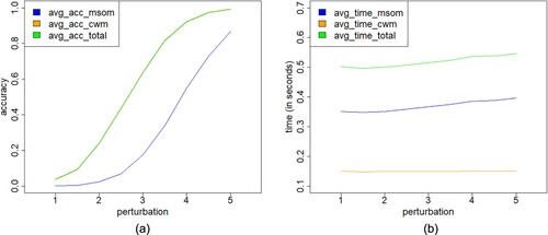is a three-dimensional vector and follows a three-variate normal distribution. We obtain the average accuracy and computational performance of the two perturbation models for detecting outliers by using the same procedure as with the VAR(1) model. From Figure 1(a), the average accuracy curve of the CWM structure does not seem to be on the graph, but this is due to the fact that such a curve overlaps with the total accuracy curve as the cases detected by the MSOM are all detected by The CWM. From Figure 1(b), the average time curve of MSOM is nearly three times as much as the CWM curve. Thus the CWM structure performs better than the MSOM in computational efficiency.

Figure 1. Plots of simulation results for the (a) average accuracy versus perturbation in the VAR(1) model with three dimensions and (b) computational performance versus perturbation of MSOM and CWM structures, for the indicated case.

4.3. VAR(3) model in two dimensions

The model parameters in Step 1 are set to generate stationary data by constructing a VAR model with lag 1 and a two-dimensional variable, on the stationarity conditions as described by e.g. [10], stated by ${\mathit{y}}_t=\mathit{v}+{\mathit{A}}_1{\mathit{y}}_{t-1}+{\mathit{A}}_2{\mathit{y}}_{t-2}+{\mathit{A}}_3{\mathit{y}}_{t-3}+{\mathit{u}}_t,$where $\begin{array}{rl}\mathit{v}& =\left(\begin{array}{c}0.0127\\ 0.0061\end{array}\right),{\mathit{A}}_1=\left(\begin{array}{cc}0& 0.1369\\ 0& 0.0852\end{array}\right),\\ {\mathit{A}}_2& =\left(\begin{array}{cc}0.0829& -0.1874\\ 0& 0\end{array}\right),{\mathit{A}}_3=\left(\begin{array}{cc}0& 0\\ 0& -0.1054\end{array}\right)\\ \mathrm{E}({\mathit{u}}_t)& =\left(\begin{array}{c}0\\ 0\end{array}\right),\mathbf{\Sigma }=\left(\begin{array}{cc}1& 0.6\\ 0.6& 1\end{array}\right),\end{array}$${\mathit{u}}_t$ 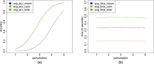is a two-dimensional vector that follows the bivariate normal distribution. The average accuracy and computational performance of two perturbation models are shown in Figure 2. From Figure 2(a), once again, the average accuracy curve of the CWM structure does not seem to be on the graph, but it overlaps with the total accuracy curve. Figures 1 and 2(a) clearly indicate that the average effect of outlier detecting increases when the size of the perturbation vector increases for both the VAR(1) and VAR(3) models. Also, the average effect of VAR(1) model is higher than that of the VAR(3) model under the same perturbation. Interestingly, the CWM structure seems to be more effective than the MSOM structure. Furthermore, although the computation time of both models is negligible, from Figure 1(b) and Figure 2(b), the CWM performs better than the MSOM, which indicates that diagnostic results of CWM may be more effective than in the MSOM. According to the simulation results, the SC test is not only valid but also significant, with its calculation being convenient and fast. However, our study suggests that these two models should be applied in combination in practical applications, because they consider the statistical diagnosis problem from different perturbation perspectives.

Figure 2. Plots of simulation results for the (a) average accuracy versus perturbation in the VAR(3) model with two dimensions and (b) computational performance versus perturbation of MSOM and CWM structures, for the indicated case.

5. Empirical study

In this section, we conduct an empirical study based on our results presented in Section 3 and compare it with local influence analysis. We choose the monthly log-returns of International Business Machines Corporation stock and the Standard & Poor's 500 index.

5.1. The data

We use International Business Machines Corporation stock (IBM) and the Standard & Poor's 500 Index (S&P500) from May 1938 to December 2008 as two-dimensional vectors to construct a VAR model and to conduct our SC test. The selection of IBM and S&P500 is mainly based on the following practical and theoretical considerations:

1. IBM is the world's largest information technology and business solutions company, and S&P500 is widely regarded as an ideal target of stock index futures contracts because of its wide sampling area, strong representativeness, high accuracy and good continuity. In addition, IBM had a weighting of more than 6 percent in S&P500 during May 1938 and December 2008, so they may influence each other.

2. There is an obvious relationship between the Student-t and normal distributions. As the degree of freedom increases, the Student-t distribution tends to be close to the normal distribution. Therefore, when the degree of freedom is large, the local influence analysis method of the Student-t distribution can be used to compare with SC test under the normal distribution.

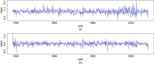
Therefore, based on the interaction between IBM and S&P500, it would be of great practical significance to construct a VAR model between them with the SC test. In addition, based on the relationship between the Student-t and normal distributions, it would be of great theoretical significance to compare the SC test under the normal distribution with local influence analysis under the Student-t distribution. For illustration purposes, we simply consider a bivariate normal distribution. Figure 3 shows the IBM and S&P500's monthly log returns from May 1938 to December 2008 (a total of 848 cases).

Figure 3. Plots of time series for (a) IBM and (b) S&P500 monthly log-returns data.

5.2. Fitting a vector autoregressive model

First, we select the order of the VAR model to be one based on Table 1 which is the result of the VARselect function of the MTS package implemented in the R software.

Table 1. Result of VARselect corresponding to the values of the Akaike (AIC) and Hannan–Quinn information (HQIC) criteria, score (SC), and final prediction error (FPE) for the IBM and S&P500 monthly log returns.

i	AIC	HQIC	SC	FPE
1	−12.1146	−12.1016	−12.0807	5.48E−06
2	−12.1128	−12.0912	−12.0563	5.49E−06
3	−12.1047	−12.0744	−12.0257	5.53E−06
4	−12.1034	−12.0644	−12.0018	5.54E−06
5	−12.1044	−12.0568	−11.9802	5.53E−06
6	−12.0971	−12.0409	−11.9503	5.58E−06
7	−12.0898	−12.0249	−11.9205	5.62E−06
8	−12.0847	−12.0112	−11.8928	5.65E−06
9	−12.0778	−11.9956	−11.8633	5.68E−06
10	−12.0687	−11.9778	−11.8316	5.74E−06

We find the estimates $\mathit{B}$ and $\mathbf{\Sigma }$ according to (8(8) $\begin{array}{rl}\hat{\mathit{B}}& =\mathit{Y}{\mathit{X}}^{\mathrm{\top }}({\mathit{X}}^{\mathrm{\top }}\mathit{X}{)}^{-1},\end{array}$(8) ) and (9(9) $\begin{array}{rl}\hat{\mathbf{\Sigma }}& =\frac{1}{T-p}\hat{\mathit{U}}{\hat{\mathit{U}}}^{\mathrm{\top }},\end{array}$(9) ) under the VAR(1) model given by (24) ${\mathit{y}}_t=\mathit{v}+\mathit{B}{\mathit{y}}_{t-1}+{\mathit{u}}_t,$(24) where $\begin{array}{rl}\mathit{v}& =\left(\begin{array}{c}0.0123\\ 0.0063\end{array}\right),\mathit{B}=\left(\begin{array}{cc}0.0041& 0.0661\\ 0.0132& -0.0103\end{array}\right),\\ \mathrm{E}({\mathit{u}}_t)& =\left(\begin{array}{c}0\\ 0\end{array}\right),\mathbf{\Sigma }=\left(\begin{array}{cc}0.0044& 0.0017\\ 0.0017& 0.0019\end{array}\right).\end{array}$In addition, we get the standardized residuals of the VAR(1) model, which are shown in Figure 4. In general, multivariate normality is based on the judgment of the marginal distributions, that is, if all marginal distributions of a multivariate distribution are normal, then the vector is considered to be multivariate normal distributed. In this case, there are very few non-normal multivariate sets. Therefore, the Kolmogorov–Smirnov test can be used to assess the normality of the residuals of each variable. Table 2 reports the test results indicating the residuals follow a multivariate normal distribution because the p-value is greater than the critical point often employed for detecting significance, that is, $\alpha =0.05$.

Figure 4. Plots of time series for standardized residuals of the VAR(1) model with (a) IBM and (b) S&P500 monthly log-returns data.

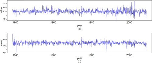
Table 2. Kolmogorov–Smirnov test for the standardized residuals of the VAR(1) model with IBM and S&P500 data.

Dataset	Statistic	p-value
IBM	0.0374	0.1819
S&P500	0.0417	0.1015

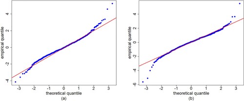
To compare the fit of the normal distribution with the empirical probability density function and the Student-t distribution curves, we standardize the data for these distributions to have the same mean and the same variance. Figure 5 gives the empirical non-parametric estimate of the probability density function of the standardized residuals, considering the normal distribution and Student-t distribution with 10 degrees of freedom. From Figure 5, we can first see that the normal distribution and Student-t distribution are almost the same. From the quantile–quantile (QQ) plot shown in Figure 6, the fitting curve deviates from the diagonal and it is obvious that one point deviates from all the points, but most cases tend to fall on the line y = x, so the residual is approximately normal distribution. Then, the two distributions seems to provide an appropriate fit. We select the normal distribution.

Figure 5. Plots of probability density functions of the standardized residuals with (a) IBM and (b) S&P500 monthly log-returns data, for the indicated method/model.

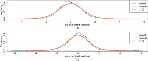
Figure 6. QQ plots of the residuals for the VAR(1) model with (a) IBM and (b) S&P500 monthly log-returns data.

5.3. SC test of the IBM and S&P500 data

According to the VAR(1) model defined in Section 5.2, we can calculate the SC statistic of the MSOM and CWM structures. Then, we can get cases exceed the benchmark whose value is ${\chi }_{0.05/848}^2(T-p)$ from the results given in (14(14) $\mathrm{SC}({\mathit{\theta }}_{10})={\left\{{\left(\frac{\mathrm{\partial }L}{\mathrm{\partial }{\mathit{\theta }}_1}\right)}^{\mathrm{\top }}{\mathcal{I}}^{11}\left(\frac{\mathrm{\partial }L}{\mathrm{\partial }{\mathit{\theta }}_1}\right)\right\}}_{{\mathit{\theta }}_1={\mathit{\theta }}_{10}}\stackrel{D}{⟶}{\chi }^2(p_1),$(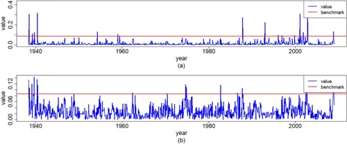14) ). The cases are considered as strong influence cases (or outliers) at the 5% significance level. Thus we calculate the SC statistics of all case points in the two perturbation models and plot them in Figure 7. The horizontal line in the figures represents the benchmark, which is a reference for detecting whether the case is abnormal. When the SC statistic exceeds the horizontal line, the case result has a significant impact, such as presented in Table 3 by the MSOM or CWM model. The symbol ‘$\ast$’ indicates that the outlier is identified by the corresponding perturbation model. We can see that the outliers identified by the CWM include the outliers identified by the MSOM. As mentioned in Section 4, the CWM is better than the MSOM.

Figure 7. Plots of values for the SC statistic and benchmark of the (a) MSOM and (b) CWM models with both IBM and S&P500 monthly log-returns data.

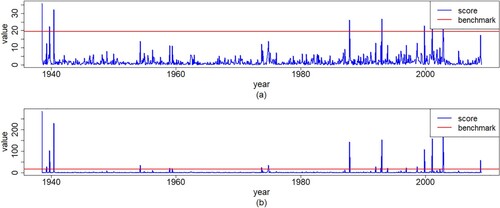
Table 3. Summary of SC test diagnostics with IBM and S&P500 data.

Date	IBM	S&P500	MSOM	CWM
1938/6/30	0.095406	0.247033	*	*
1939/3/31	−0.034057	−0.135433		*
1939/9/30	−0.014749	0.16458	*	*
1940/5/31	−0.161796	−0.239541	*	*
1954/3/31	0.232472	0.03021		*
1958/12/31	0.22679	0.05202		*
1959/5/29	0.204352	0.018927		*
1973/9/28	−0.142857	0.040096		*
1974/10/31	0.189465	0.163047		*
1987/10/30	−0.187396	−0.21763	*	*
1991/12/31	−0.037838	0.111588		*
1992/10/30	−0.171827	0.002106		*
1992/12/31	−0.261905	0.010108	*	*
1993/11/30	0.17663	−0.012911		*
1996/11/29	0.238178	0.073376		*
1998/8/31	−0.14834	−0.145797		*
1999/10/29	−0.188017	0.062539	*	*
2001/1/31	0.317647	0.034637	*	*
2002/9/30	−0.226453	−0.110013		*
2002/10/31	0.353799	0.086436	*	*
2008/10/31	−0.205113	−0.169425		*

5.4. Modified data analysis

Next, we present a new VAR model given in (25(25) ${\mathit{y}}_t=\mathit{v}+\mathit{B}{\mathit{y}}_{t-1}+{\mathit{u}}_t,$(25) ) after deleting the outliers identified in Section 5.3. The lag order of the new model is still one by using the AIC and BIC. The standardized residuals obtained after remodelling are shown in Figure 8. Then, the new VAR model is given by (25) ${\mathit{y}}_t=\mathit{v}+\mathit{B}{\mathit{y}}_{t-1}+{\mathit{u}}_t,$(25) where $\mathit{v}=\left(\begin{array}{c}0.0115\\ 0.0059\end{array}\right),\mathit{B}=\left(\begin{array}{cc}0.0883& -0.0251\\ 0.0441& -0.0184\end{array}\right),\mathrm{E}({\mathit{u}}_t)=\left(\begin{array}{c}0\\ 0\end{array}\right),\mathbf{\Sigma }=\left(\begin{array}{cc}0.0035& 0.0014\\ 0.0014& 0.0015\end{array}\right).$Comparing Figures 4 and 8, we find that the standardized residuals of the VAR(1) model have almost no extreme values and are more stable. From Table 4, we see that the residuals of the VAR(1) model still pass the multivariate normal distribution test, which is a very positive signal. In Figure 9, the kernel density curves of the residuals and the normal density almost overlap, and the effect is better than that in Figure 5. The QQ plot of the IBM and S&P500 data shown in Figure 10 is also better than that in Figure 6, and the points are more clearly distributed on the y = x line.

Figure 8. Plots of standardized residuals for the new VAR(1) model with (a) IBM and (b) S&P500 monthly log-returns data.

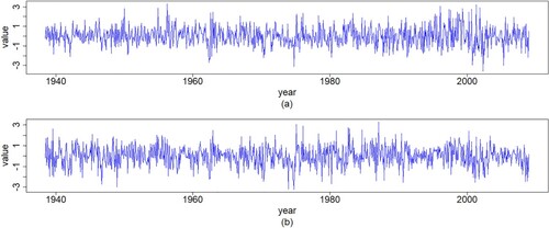
Figure 9. Plots of probability density functions of the standardized residuals with (a) IBM and (b) S&P500 monthly log-returns data, for the indicated method/model.

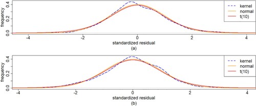
Figure 10. QQ plots of the residuals for the new VAR(1) model with (a) IBM and (b) S&P500 monthly log-returns data.

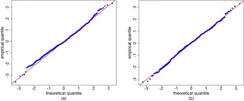
Table 4. Kolmogorov–Smirnov test for the standardized residuals of the new VAR(1) model with IBM and S&P500 data.

Dataset	Statistic	p-value
IBM	0.0335	0.29190
S&P500	0.03604	0.2158

5.5. Comparison between SC test and local influence analyses

Next, we compare the result of Table 3 with those presented in [5,6] (see Table 5) to analyse the effect of two methods.

Table 5. Summary of the curvature-based diagnostics with log returns data for case-weights and data perturbations.

Date	IBM	S&P500	CW	Data	Date	IBM	S&P500	CW	Data
1938/5/31	0.017986	−0.04433		*	1974/10/31	0.189465	0.163047		*
1938/6/30	0.095406	0.247033	*		1982/9/30	0.04078	0.007614		*
1938/7/30	0.065147	0.072664		*	1986/8/29	0.055472	0.071193		*
1939/2/28	0.037298	0.03252		*	1987/9/30	−0.104677	−0.024166		*
1939/3/31	−0.034057	−0.135433	*		1987/10/30	−0.187396	−0.21763	*
1939/6/30	−0.003529	−0.063793		*	1992/12/31	−0.261905	0.010108	*
1939/8/31	−0.093583	−0.071429		*	1996/1/31	0.187414	0.032617	*
1939/9/30	−0.014749	0.16458	*		1996/11/29	0.238178	0.073376	*
1940/4/30	−0.013361	−0.004898		*	1999/10/29	−0.188017	0.062539	*
1940/5/31	−0.161796	−0.239541	*		2001/1/31	0.317647	0.034637	*
1940/6/29	−0.047619	0.076591		*	2001/10/31	0.17826	0.018099	*
1948/10/30	0.080702	0.067786		*	2002/5/31	−0.037727	−0.009081		*
1954/3/31	0.232472	0.03021	*		2002/8/30	0.072869	0.004881		*
1958/12/31	0.22679	0.05202	*		2002/10/31	0.353799	0.086436	*
1959/5/29	0.204352	0.018927	*		2008/9/30	−0.039185	−0.090791		*
1962/5/31	−0.133811	−0.08599		*	2008/10/31	−0.205113	−0.169425	*	*
1970/5/29	−0.063087	−0.060967		*	2008/11/28	−0.116919	−0.074849		*
1974/8/30	−0.040298	−0.090279		*

When the degrees of freedom of the Student-t distribution becomes large enough, this distribution is equivalent to the normal one. Therefore, the result of local influence analysis is obtained under the Student-t distribution such as in [6] or the normal distribution as in [5]. For this reason, the method of [5] can also be used to diagnose the data in Section 5. Employing the bivariate VAR(1) model built in Section 5.2, we calculate the corresponding diagnostic vector and find $2.5/\sqrt{T}$ as the empirical benchmark being the best through many experiments.

The horizontal line represents the empirical benchmark that determines whether a case is significantly influential in Figure 11. The case is significantly influential when its diagnostic value is beyond the horizontal lines such as reported in Table 5. It tallies the cases that are identified as influential for both IBM and S&P500 data, and again the symbol '$\ast$' indicates that the outlier is identified through the perturbation of case-weights and data. Note that the cases indicated in Tables 3 and 5 actually correspond to certain material historical events. All these cases are concentrated in and after the 2008 financial crisis.

Figure 11. Plots of values for diagnostic vectors of (a) case-weights and (b) data perturbations with both IBM and S&P500 monthly log-returns data.

Interestingly, 71% of the SC test findings is exactly the same as those identified by the local influence analysis. It strongly illustrates that both methods are powerful to identify extreme cases including influential cases or outliers. The SC test and the local influence methods do detect different cases. The SC test identifies six outliers that the local influence method does not, while the local influence method detects five influential cases that the SC test does not. The local influence method can detect continuous-time extreme values, while the SC test is more accurate for the other cases. The benchmark of the SC test is dependent on the significance level, which may have statistical implications, while the local influence analysis can detect influential cases, which are not necessarily outliers. To conclude, the SC test method is indeed effective as used in [35].

6. Concluding remarks

In this paper, we have studied statistical diagnostics based on the score test with a vector autoregressive model under normal distributions. We have derived the information matrix under the mean-shift perturbation and case-weight perturbation models, and obtained their corresponding score statistics. Then, building the three-dimensional and two-dimensional vector autoregressive models, we have examined the effectiveness of the mean-shift and the case-weight perturbations. In addition, we have made an empirical analysis for the logarithm of the weekly returns of IBM and S&P500 from May 1938 to December 2008. After deleting those outliers identified, our updated model is better than the original model. We have also compared our results with those by the local influence analysis. Finally, we have concluded that the score test method is effective.

Acknowledgements

We would like to thank the Editors and Reviewers very much for their insightful and constructive comments which led to an improved presentation of the manuscript. The research of Y. Liu was supported by the National Social Science Fund of China [grant No. 19BTJ036]. The research of V. Leiva was partially funded by the National Agency for Research and Development (ANID) [project grant number FONDECYT 1200525] of the Chilean government under the Ministry of Science, Technology, Knowledge, and Innovation.

Disclosure statement

No potential conflict of interest was reported by the author(s).

Appendix

Based on the matrix differential calculus developed and used in, e.g. [14,38,39], we establish the results.

A.1. Proof of Theorem 3.1

Proof.

For Equation (19(19) $\begin{array}{rl}& =-\frac{(T-p)p_1}{2}\log (2\pi )-\frac{(T-p)}{2}\log |\mathbf{\Sigma }|-\frac{1}{2}({\mathit{y}}_i-\mathit{B}{\mathit{x}}_i-\mathit{\gamma }{)}^{\mathrm{\top }}{\mathbf{\Sigma }}^{-1}({\mathit{y}}_i-\mathit{B}{\mathit{x}}_i-\mathit{\gamma })\\ & -\frac{1}{2}[{\mathit{y}}_{(i)}-({\mathit{X}}_{(i)}^{\mathrm{\top }}\otimes {\mathit{I}}_{p_1})\mathit{\beta }{]}^{\mathrm{\top }}[{\mathit{I}}_{T-p-1}\otimes {\mathbf{\Sigma }}^{-1}][{\mathit{y}}_{(i)}-({\mathit{X}}_{(i)}^{\mathrm{\top }}\otimes {\mathit{I}}_{p_1})\mathit{\beta }],\end{array}$(19) ), we obtain $\begin{array}{rl}{d}_{\gamma }L(\theta )& =\frac{1}{2}(y_i-B{x}_i-\gamma {)}^{\mathrm{\top }}{\mathbf{\Sigma }}^{-1}\mathrm{d}\gamma +\frac{1}{2}\mathrm{d}{\gamma }^{\mathrm{\top }}{\mathbf{\Sigma }}^{-1}(y_i-B{x}_i-\gamma )\\ & =\mathrm{d}{\gamma }^{\mathrm{\top }}{\mathbf{\Sigma }}^{-1}(y_i-B{x}_i-\gamma )\end{array}$so $\frac{\mathrm{\partial }L(\theta )}{\mathrm{\partial }\gamma }={\mathbf{\Sigma }}^{-1}(y_i-B{x}_i-\gamma )$and with regard to $d_{\gamma }L(\theta )$, we obtain that $d_{\gamma {\gamma }^{\mathrm{\top }}}L(\theta )=-\mathrm{d}{\gamma }^{\mathrm{\top }}{\mathbf{\Sigma }}^{-1}\mathrm{d}\gamma$Therefore, we acquire that $\frac{{\mathrm{\partial }}^{2}L(\theta )}{\mathrm{\partial }\gamma \mathrm{\partial }{\gamma }^{\mathrm{\top }}}=-{\mathbf{\Sigma }}^{-1}$By $d_{\gamma }L(\theta )$, in the same way, we attain that $\begin{array}{rl}{d}_{\gamma {\beta }^{\mathrm{\top }}}L(\theta )& =d[\mathrm{d}{\gamma }^{\mathrm{\top }}{\mathbf{\Sigma }}^{-1}(y_i-B{x}_i-\gamma )]=d[\mathrm{d}{\gamma }^{\mathrm{\top }}{\mathbf{\Sigma }}^{-1}(y_i-(x_i^{\mathrm{\top }}\otimes I_K)\beta -\gamma )]\\ & =\mathrm{d}{\gamma }^{\mathrm{\top }}[-{\mathbf{\Sigma }}^{-1}(x_i^{\mathrm{\top }}\otimes I_K)]\mathrm{d}\beta \end{array}$Then $\frac{{\mathrm{\partial }}^{2}L(\theta )}{\mathrm{\partial }\gamma \mathrm{\partial }{\beta }^{\mathrm{\top }}}=-{\mathbf{\Sigma }}^{-1}(x_i^{\mathrm{\top }}\otimes I_K)$By $d_{\gamma }L(\theta )$, we get that $\begin{array}{rl}{d}_{\gamma s^{\mathrm{\top }}}L(\theta )& =d[\mathrm{d}{\gamma }^{\mathrm{\top }}{\mathbf{\Sigma }}^{-1}(y_i-B{x}_i-\gamma )]=\mathrm{d}{\gamma }^{\mathrm{\top }}d({\mathbf{\Sigma }}^{-1})(y_i-B{x}_i-\gamma )\\ & =-\mathrm{d}{\gamma }^{\mathrm{\top }}{\mathbf{\Sigma }}^{-1}d\mathbf{\Sigma }{\mathbf{\Sigma }}^{-1}(y_i-B{x}_i-\gamma )=-{\mu }_i^{\mathrm{\top }}{\mathbf{\Sigma }}^{-1}d\mathbf{\Sigma }{\mathbf{\Sigma }}^{-1}\mathrm{d}\gamma \\ & =-\mathrm{tr}({\mu }_i^{\mathrm{\top }}{\mathbf{\Sigma }}^{-1}d\mathbf{\Sigma }{\mathbf{\Sigma }}^{-1}\mathrm{d}\gamma )=-(\text{v}ecd\mathbf{\Sigma }{)}^{\mathrm{\top }}({\mathbf{\Sigma }}^{-1}{\mu }_i)\otimes {\mathbf{\Sigma }}^{-1}\mathrm{d}\gamma \\ & =-(D_K\mathrm{vech}d\mathbf{\Sigma }{)}^{\mathrm{\top }}({\mathbf{\Sigma }}^{-1}{\mu }_i)\otimes {\mathbf{\Sigma }}^{-1}\mathrm{d}\gamma \\ & =[d(\mathrm{vech}\mathbf{\Sigma }{)}^{\mathrm{\top }}][-D_k^{\mathrm{\top }}({\mathbf{\Sigma }}^{-1}{\mu }_i)\otimes {\mathbf{\Sigma }}^{-1}]\mathrm{d}\gamma \\ & =\mathrm{d}{\gamma }^{\mathrm{\top }}[-({\mu }_i^{\mathrm{\top }}{\mathbf{\Sigma }}^{-1})\otimes {\mathbf{\Sigma }}^{-1}{D}_k]d(\text{v}ech\mathbf{\Sigma })=\mathrm{d}{\gamma }^{\mathrm{\top }}[-({\mu }_i^{\mathrm{\top }}{\mathbf{\Sigma }}^{-1})\otimes {\mathbf{\Sigma }}^{-1}{D}_k]\mathrm{d}s\end{array}$So $\frac{{\mathrm{\partial }}^{2}L(\theta )}{\mathrm{\partial }\gamma \mathrm{\partial }{s}^{\mathrm{\top }}}=-({\mu }_i^{\mathrm{\top }}{\mathbf{\Sigma }}^{-1})\otimes {\mathbf{\Sigma }}^{-1}{D}_k$Taking equation (19(19) $\begin{array}{rl}& =-\frac{(T-p)p_1}{2}\log (2\pi )-\frac{(T-p)}{2}\log |\mathbf{\Sigma }|-\frac{1}{2}({\mathit{y}}_i-\mathit{B}{\mathit{x}}_i-\mathit{\gamma }{)}^{\mathrm{\top }}{\mathbf{\Sigma }}^{-1}({\mathit{y}}_i-\mathit{B}{\mathit{x}}_i-\mathit{\gamma })\\ & -\frac{1}{2}[{\mathit{y}}_{(i)}-({\mathit{X}}_{(i)}^{\mathrm{\top }}\otimes {\mathit{I}}_{p_1})\mathit{\beta }{]}^{\mathrm{\top }}[{\mathit{I}}_{T-p-1}\otimes {\mathbf{\Sigma }}^{-1}][{\mathit{y}}_{(i)}-({\mathit{X}}_{(i)}^{\mathrm{\top }}\otimes {\mathit{I}}_{p_1})\mathit{\beta }],\end{array}$(19) ) into consideration, we obtain $\begin{array}{rl}{d}_{\beta }L(\theta )& =\frac{1}{2}[({\dot{X}}^{\mathrm{\top }}\otimes I_K)\mathrm{d}\beta {]}^{\mathrm{\top }}(I_{T-p-1}\otimes {\mathbf{\Sigma }}^{-1})[\dot{y}-({\dot{X}}^{\mathrm{\top }}\otimes I_K)\beta ]\\ & +\frac{1}{2}[\dot{y}-({\dot{X}}^{\mathrm{\top }}\otimes I_K)\beta {]}^{\mathrm{\top }}(I_{T-p-1}\otimes {\mathbf{\Sigma }}^{-1})({\dot{X}}^{\mathrm{\top }}\otimes I_K)\mathrm{d}\beta \\ & -\frac{1}{2}d[y_i-(x_i^{\mathrm{\top }}\otimes I_K)\beta -\gamma {]}^{\mathrm{\top }}{\mathbf{\Sigma }}^{-1}[y_i-(x_i^{\mathrm{\top }}\otimes I_K)\beta -\gamma ]\\ & =\mathrm{d}{\beta }^{\mathrm{\top }}(\dot{X}\otimes I_K)(I_{T-p-1}\otimes {\mathbf{\Sigma }}^{-1})\dot{\mu }+\frac{1}{2}[(x_i^{\mathrm{\top }}\otimes I_K)\mathrm{d}\beta {]}^{\mathrm{\top }}{\mathbf{\Sigma }}^{-1}{\mu }_i\\ & +\frac{1}{2}{\mu }_i^{\mathrm{\top }}{\mathbf{\Sigma }}^{-1}(x_i^{\mathrm{\top }}\otimes I_K)\mathrm{d}\beta \\ & =\mathrm{d}{\beta }^{\mathrm{\top }}(\dot{X}\otimes {\mathbf{\Sigma }}^{-1})\dot{\mu }+\mathrm{d}{\beta }^{\mathrm{\top }}(x_i\otimes I_K){\mathbf{\Sigma }}^{-1}{\mu }_i\\ & =\mathrm{d}{\beta }^{\mathrm{\top }}(\dot{X}\otimes {\mathbf{\Sigma }}^{-1})[\dot{y}-({\dot{X}}^{\mathrm{\top }}\otimes I_K)\beta ]\\ & +\mathrm{d}{\beta }^{\mathrm{\top }}(x_i\otimes I_K){\mathbf{\Sigma }}^{-1}[y_i-(x_i^{\mathrm{\top }}\otimes I_K)\beta -\gamma ]\end{array}$From $d_{\beta }L(\theta )$, we deduce that $\begin{array}{rl}{d}_{\beta {\gamma }^{\mathrm{\top }}}L(\theta )& =d[\mathrm{d}{\beta }^{\mathrm{\top }}(x_i\otimes I_K){\mathbf{\Sigma }}^{-1}[y_i-(x_i^{\mathrm{\top }}\otimes I_K)\beta -\gamma ]]\\ & =\mathrm{d}{\beta }^{\mathrm{\top }}[-(x_i\otimes I_K){\mathbf{\Sigma }}^{-1}]\mathrm{d}\gamma \end{array}$So we gain that $\frac{{\mathrm{\partial }}^{2}L(\theta )}{\mathrm{\partial }\beta \mathrm{\partial }{\gamma }^{\mathrm{\top }}}=-(x_i\otimes I_K){\mathbf{\Sigma }}^{-1}$By considering $d_{\beta }L(\theta )$, in the same way, we attain that $\begin{array}{rl}{d}_{\beta {\beta }^{\mathrm{\top }}}L(\theta )& =-\mathrm{d}{\beta }^{\mathrm{\top }}(\dot{X}\otimes {\mathbf{\Sigma }}^{-1})({\dot{X}}^{\mathrm{\top }}\otimes I_K)\mathrm{d}\beta -\mathrm{d}{\beta }^{\mathrm{\top }}(x_i\otimes I_K){\mathbf{\Sigma }}^{-1}(x_i^{\mathrm{\top }}\otimes I_K)\mathrm{d}\beta \\ & =\mathrm{d}{\beta }^{\mathrm{\top }}[-(\dot{X}{\dot{X}}^{\mathrm{\top }})\otimes {\mathbf{\Sigma }}^{-1}]\mathrm{d}\beta +\mathrm{d}{\beta }^{\mathrm{\top }}[-(x_i{x}_i^{\mathrm{\top }})\otimes {\mathbf{\Sigma }}^{-1}]\mathrm{d}\beta \\ & =\mathrm{d}{\beta }^{\mathrm{\top }}[-(X{X}^{\mathrm{\top }})\otimes {\mathbf{\Sigma }}^{-1}]\mathrm{d}\beta \end{array}$Thereby we arrive that $\frac{{\mathrm{\partial }}^{2}L(\theta )}{\mathrm{\partial }\beta \mathrm{\partial }{\beta }^{\mathrm{\top }}}=-(X{X}^{\mathrm{\top }})\otimes {\mathbf{\Sigma }}^{-1}$Another form of $d_{\beta s^{\mathrm{\top }}}L(\theta )$ should be applied due to deriving $d_{\beta }L(\theta )$. By Equation (18(18) $\begin{array}{rl}& =-\frac{(T-p)p_1}{2}\log (2\pi )-\frac{(T-p)}{2}\log |\mathbf{\Sigma }|-\frac{1}{2}({\mathit{y}}_i-\mathit{B}{\mathit{x}}_i-\mathit{\gamma }{)}^{\mathrm{\top }}{\mathbf{\Sigma }}^{-1}({\mathit{y}}_i-\mathit{B}{\mathit{x}}_i-\mathit{\gamma })\\ & -\frac{1}{2}\mathrm{tr}[({\mathit{Y}}_{(i)}-\mathit{B}\mathit{X}{)}_{(i)}^{\mathrm{\top }}{\mathbf{\Sigma }}^{-1}({\mathit{Y}}_{(i)}-\mathit{B}{\mathit{X}}_{(i)})]\end{array}$(18) ), we know that $\begin{array}{rl}{d}_{\beta }L(\theta )& =-\frac{1}{2}d[\mathrm{tr}((\dot{Y}-B\dot{X}{)}^{\mathrm{\top }}{\mathbf{\Sigma }}^{-1}(\dot{Y}-B\dot{X}))]\\ & -\frac{1}{2}d[(y_i-B{x}_i-\gamma {)}^{\mathrm{\top }}{\mathbf{\Sigma }}^{-1}(y_i-B{x}_i-\gamma )]\\ & =\frac{1}{2}\mathrm{tr}[(dB\dot{X}{)}^{\mathrm{\top }}{\mathbf{\Sigma }}^{-1}(\dot{Y}-B\dot{X})]+\frac{1}{2}\mathrm{tr}[(\dot{Y}-B\dot{X}{)}^{\mathrm{\top }}{\mathbf{\Sigma }}^{-1}(dB\dot{X})]\\ & +\frac{1}{2}[dB{x}_i){]}^{\mathrm{\top }}{\mathbf{\Sigma }}^{-1}(y_i-B{x}_i-\gamma )+\frac{1}{2}(y_i-B{x}_i-\gamma {)}^{\mathrm{\top }}{\mathbf{\Sigma }}^{-1}dB{x}_i\\ & =\frac{1}{2}\mathrm{tr}[{\dot{X}}^{\mathrm{\top }}d{B}^{\mathrm{\top }}\mathbf{\Sigma }-1(\dot{Y}-B\dot{X})]+\frac{1}{2}\mathrm{tr}[(\dot{Y}-B\dot{X}{)}^{\mathrm{\top }}\mathbf{\Sigma }-1dB\dot{X}]\\ & +\mathrm{tr}[x_i^{\mathrm{\top }}d{B}^{\mathrm{\top }}{\mathbf{\Sigma }}^{-1}(y_i-B{x}_i-\gamma )]\\ & =\mathrm{tr}[{\dot{X}}^{\mathrm{\top }}d{B}^{\mathrm{\top }}{\mathbf{\Sigma }}^{-1}(\dot{Y}-B\dot{X})]+\mathrm{tr}[x_i^{\mathrm{\top }}d{B}^{\mathrm{\top }}\mathbf{\Sigma }-1(y_i-B{x}_i-\gamma )]\end{array}$Through $d_{\beta }L(\theta )$, we obtain that $\begin{array}{rl}{d}_{\beta s^{\mathrm{\top }}}L(\theta )& =-\mathrm{tr}[{\dot{X}}^{\mathrm{\top }}d{B}^{\mathrm{\top }}{\mathbf{\Sigma }}^{-1}d\mathbf{\Sigma }{\mathbf{\Sigma }}^{-1}(\dot{Y}-B\dot{X})]-\mathrm{tr}[x_i^{\mathrm{\top }}d{B}^{\mathrm{\top }}{\mathbf{\Sigma }}^{-1}d\mathbf{\Sigma }{\mathbf{\Sigma }}^{-1}(y_i-B{x}_i-\gamma )]\\ & =-\mathrm{tr}[({\mathbf{\Sigma }}^{-1}dB\dot{X}{)}^{\mathrm{\top }}d\mathbf{\Sigma }{\mathbf{\Sigma }}^{-1}(\dot{Y}-B\dot{X})]\\ & -\mathrm{tr}[({\mathbf{\Sigma }}^{-1}dB{x}_i{)}^{\mathrm{\top }}d\mathbf{\Sigma }{\mathbf{\Sigma }}^{-1}(y_i-B{x}_i-\gamma )]\\ & =-[\mathrm{vec}({\mathbf{\Sigma }}^{-1}dB\dot{X}){]}^{\mathrm{\top }}\mathrm{vec}[d\mathbf{\Sigma }{\mathbf{\Sigma }}^{-1}(\dot{Y}-B\dot{X})]\\ & -[\mathrm{vec}({\mathbf{\Sigma }}^{-1}dB{x}_i){]}^{\mathrm{\top }}\mathrm{vec}[d\mathbf{\Sigma }{\mathbf{\Sigma }}^{-1}(y_i-B{x}_i-\gamma )]\\ & =-[({\dot{X}}^{\mathrm{\top }}\otimes {\mathbf{\Sigma }}^{-1})\mathrm{d}\beta {]}^{\mathrm{\top }}[({\mathbf{\Sigma }}^{-1}(\dot{Y}-B\dot{X}){)}^{\mathrm{\top }}\otimes I_K]d(\mathrm{vec}\mathbf{\Sigma })\\ & -[(x_i^{\mathrm{\top }}\otimes {\mathbf{\Sigma }}^{-1})\mathrm{d}\beta {]}^{\mathrm{\top }}[{\mathbf{\Sigma }}^{-1}(y_i-B{x}_i-\gamma ){]}^{\mathrm{\top }}\otimes I_{K}d(\mathrm{vec}\mathbf{\Sigma })\\ & =-\mathrm{d}{\beta }^{\mathrm{\top }}(\dot{x}\otimes {\mathbf{\Sigma }}^{-1})[({\dot{U}}^{\mathrm{\top }}{\mathbf{\Sigma }}^{-1})\otimes I_K]D_{K}d(\mathrm{vech}\mathbf{\Sigma })\\ & -\mathrm{d}{\beta }^{\mathrm{\top }}(x_i\otimes {\mathbf{\Sigma }}^{-1})[(u_i^{\mathrm{\top }}{\mathbf{\Sigma }}^{-1})\otimes I_K]D_{K}d(\mathrm{vech}\mathbf{\Sigma })\\ & =\mathrm{d}{\beta }^{\mathrm{\top }}[-(\dot{X}{\dot{U}}^{\mathrm{\top }}{\mathbf{\Sigma }}^{-1})\otimes {\mathbf{\Sigma }}^{-1}]D_{K}d(\mathrm{vech}\mathbf{\Sigma })\\ & +\mathrm{d}{\beta }^{\mathrm{\top }}[-(x_i{u}_i^{\mathrm{\top }}{\mathbf{\Sigma }}^{-1})\otimes {\mathbf{\Sigma }}^{-1}]D_{K}d(\mathrm{vech}\mathbf{\Sigma })\\ & =\mathrm{d}{\beta }^{\mathrm{\top }}[-(\dot{X}{\dot{U}}^{\mathrm{\top }}{\mathbf{\Sigma }}^{-1})\otimes {\mathbf{\Sigma }}^{-1}]D_{K}ds+\mathrm{d}{\beta }^{\mathrm{\top }}[-(x_i{u}_i^{\mathrm{\top }}{\mathbf{\Sigma }}^{-1})\otimes {\mathbf{\Sigma }}^{-1}]D_{K}ds\\ & =\mathrm{d}{\beta }^{\mathrm{\top }}[-(X{U}^{\mathrm{\top }}{\mathbf{\Sigma }}^{-1})\otimes {\mathbf{\Sigma }}^{-1}]D_{K}ds\end{array}$Then, we get that $\frac{{\mathrm{\partial }}^{2}L(\theta )}{\mathrm{\partial }\beta \mathrm{\partial }{s}^{\mathrm{\top }}}=-[(X{U}^{\mathrm{\top }}{\mathbf{\Sigma }}^{-1})\otimes {\mathbf{\Sigma }}^{-1}]D_K$According to Equation (18(18) $\begin{array}{rl}& =-\frac{(T-p)p_1}{2}\log (2\pi )-\frac{(T-p)}{2}\log |\mathbf{\Sigma }|-\frac{1}{2}({\mathit{y}}_i-\mathit{B}{\mathit{x}}_i-\mathit{\gamma }{)}^{\mathrm{\top }}{\mathbf{\Sigma }}^{-1}({\mathit{y}}_i-\mathit{B}{\mathit{x}}_i-\mathit{\gamma })\\ & -\frac{1}{2}\mathrm{tr}[({\mathit{Y}}_{(i)}-\mathit{B}\mathit{X}{)}_{(i)}^{\mathrm{\top }}{\mathbf{\Sigma }}^{-1}({\mathit{Y}}_{(i)}-\mathit{B}{\mathit{X}}_{(i)})]\end{array}$(18) ), we have that $\begin{array}{rl}{d}_{s}L(\theta )& =-\frac{T-p}{2}d(\log |\mathbf{\Sigma }|)+d[-\frac{1}{2}\mathrm{tr}((\dot{Y}-B\dot{X}{)}^{\mathrm{\top }}{\mathbf{\Sigma }}^{-1}(\dot{Y}-B\dot{X}))]\\ & +d[-\frac{1}{2}\mathrm{tr}((y_i-B{x}_i-\gamma {)}^{\mathrm{\top }}{\mathbf{\Sigma }}^{-1}(y_i-B{x}_i-\gamma ))]\\ & =-\frac{T-p}{2}d(\log |\mathbf{\Sigma }|)+\frac{1}{2}\mathrm{tr}({\dot{U}}^{\mathrm{\top }}{\mathbf{\Sigma }}^{-1}d\mathbf{\Sigma }{\mathbf{\Sigma }}^{-1}\dot{U})+\frac{1}{2}\mathrm{tr}(u_i^{\mathrm{\top }}{\mathbf{\Sigma }}^{-1}d\mathbf{\Sigma }{\mathbf{\Sigma }}^{-1}{u}_i)\\ & =-\frac{T-p}{2}\mathrm{tr}({\mathbf{\Sigma }}^{-1}d\mathbf{\Sigma })+\frac{1}{2}\mathrm{tr}({\dot{U}}^{\mathrm{\top }}{\mathbf{\Sigma }}^{-1}d\mathbf{\Sigma }{\mathbf{\Sigma }}^{-1}\dot{U})+\frac{1}{2}\mathrm{tr}(u_i^{\mathrm{\top }}{\mathbf{\Sigma }}^{-1}d\mathbf{\Sigma }{\mathbf{\Sigma }}^{-1}{u}_i)\end{array}$We gain that, by $d_{s}L(\theta )$, $\begin{array}{rl}{d}_{s{\gamma }^{\mathrm{\top }}}L(\theta )& =d[\frac{1}{2}\mathrm{tr}((y_i-B{x}_i-\gamma {)}^{\mathrm{\top }}{\mathbf{\Sigma }}^{-1}d\mathbf{\Sigma }{\mathbf{\Sigma }}^{-1}(y_i-B{x}_i-\gamma ))]\\ & =-\frac{1}{2}\mathrm{tr}[\mathrm{d}{\gamma }^{\mathrm{\top }}{\mathbf{\Sigma }}^{-1}d\mathbf{\Sigma }{\mathbf{\Sigma }}^{-1}(y_i-B{x}_i-\gamma )]\\ & -\frac{1}{2}\mathrm{tr}[(y_i-B{x}_i-\gamma {)}^{\mathrm{\top }}{\mathbf{\Sigma }}^{-1}d\mathbf{\Sigma }{\mathbf{\Sigma }}^{-1}\mathrm{d}\gamma ]\\ & =-\mathrm{tr}[(y_i-B{x}_i-\gamma {)}^{\mathrm{\top }}{\mathbf{\Sigma }}^{-1}d\mathbf{\Sigma }{\mathbf{\Sigma }}^{-1}\mathrm{d}\gamma ]\\ & =-(\mathrm{vec}d\mathbf{\Sigma }{)}^{\mathrm{\top }}[{\mathbf{\Sigma }}^{\mathrm{\top }}(y_i-B{x}_i-\gamma )]\otimes {\mathbf{\Sigma }}^{-1}\mathrm{d}\gamma \\ & =[d(\mathrm{vech}\mathbf{\Sigma }){]}^{\mathrm{\top }}[-D_k^{\mathrm{\top }}({\mathbf{\Sigma }}^{-1}{u}_i)\otimes {\mathbf{\Sigma }}^{-1}]\mathrm{d}\gamma =\mathrm{d}{s}^{\mathrm{\top }}[-D_k^{\mathrm{\top }}({\mathbf{\Sigma }}^{-1}{u}_i)\otimes {\mathbf{\Sigma }}^{-1}]\mathrm{d}\gamma \end{array}$Thus we have $\frac{{\mathrm{\partial }}^{2}L(\theta )}{\mathrm{\partial }s\mathrm{\partial }{\gamma }^{\mathrm{\top }}}=-D_k^{\mathrm{\top }}({\mathbf{\Sigma }}^{-1}{u}_i)\otimes {\mathbf{\Sigma }}^{-1}$By $d_{s}L(\theta )$, we have that $\begin{array}{rl}{d}_{s{\beta }^{\mathrm{\top }}}L(\theta )& =\frac{1}{2}d[\mathrm{tr}((\dot{Y}-B\dot{X}{)}^{\mathrm{\top }}{\mathbf{\Sigma }}^{-1}d\mathbf{\Sigma }{\mathbf{\Sigma }}^{-1}(\dot{Y}-B\dot{X}))]\\ & +\frac{1}{2}d[\mathrm{tr}((y_i-B{x}_i-\gamma {)}^{\mathrm{\top }}{\mathbf{\Sigma }}^{-1}d\mathbf{\Sigma }{\mathbf{\Sigma }}^{-1}(y_i-B{x}_i-\gamma ))]\\ & =-\frac{1}{2}\mathrm{tr}[(d(B)\dot{X}{)}^{\mathrm{\top }}{\mathbf{\Sigma }}^{-1}d\mathbf{\Sigma }{\mathbf{\Sigma }}^{-1}(\dot{Y}-B\dot{X})]\\ & -\frac{1}{2}\mathrm{tr}[(\dot{Y}-B\dot{X}{)}^{\mathrm{\top }}{\mathbf{\Sigma }}^{-1}d\mathbf{\Sigma }{\mathbf{\Sigma }}^{-1}d(B)\dot{X}]\\ & -\frac{1}{2}\mathrm{tr}[(d(B)x_i{)}^{\mathrm{\top }}{\mathbf{\Sigma }}^{-1}d\mathbf{\Sigma }{\mathbf{\Sigma }}^{-1}(y_i-B{x}_i-\gamma )]\\ & -\frac{1}{2}\mathrm{tr}[(y_i-B{x}_i-\gamma {)}^{\mathrm{\top }}{\mathbf{\Sigma }}^{-1}d\mathbf{\Sigma }{\mathbf{\Sigma }}^{-1}d(B)x_i]\\ & =-\mathrm{tr}[{\dot{U}}^{\mathrm{\top }}{\mathbf{\Sigma }}^{-1}d\mathbf{\Sigma }{\mathbf{\Sigma }}^{-1}dB\dot{X}]-\mathrm{tr}[u_i^{\mathrm{\top }}{\mathbf{\Sigma }}^{-1}d\mathbf{\Sigma }{\mathbf{\Sigma }}^{-1}dB{x}_i]\\ & =-\mathrm{tr}[(d\mathbf{\Sigma }{\mathbf{\Sigma }}^{-1}\dot{U}{)}^{\mathrm{\top }}{\mathbf{\Sigma }}^{-1}dB\dot{X}]-\mathrm{tr}[(d\mathbf{\Sigma }{\mathbf{\Sigma }}^{\mathrm{\top }}{u}_i{)}^{\mathrm{\top }}{\mathbf{\Sigma }}^{-1}dB{x}_i]\\ & =-(\mathrm{vec}(d\mathbf{\Sigma }{\mathbf{\Sigma }}^{-1}\dot{U}){)}^{\mathrm{\top }}\mathrm{vec}({\mathbf{\Sigma }}^{-1}dB\dot{X})-(\mathrm{vec}(d\mathbf{\Sigma }{\mathbf{\Sigma }}^{\mathrm{\top }}{u}_i){)}^{\mathrm{\top }}\mathrm{vec}({\mathbf{\Sigma }}^{-1}dB{x}_i)\\ & =-((({\mathbf{\Sigma }}^{-1}\dot{U}{)}^{\mathrm{\top }}\otimes I_K)d(\mathrm{vec}\mathbf{\Sigma }){)}^{\mathrm{\top }}({\dot{X}}^{\mathrm{\top }}\otimes {\mathbf{\Sigma }}^{-1})\mathrm{d}\beta \\ & -((({\mathbf{\Sigma }}^{-1}{u}_i{)}^{\mathrm{\top }}\otimes I_K)d(\mathrm{vec}\mathbf{\Sigma }){)}^{\mathrm{\top }}(x_i^{\mathrm{\top }}\otimes {\mathbf{\Sigma }}^{-1})\mathrm{d}\beta \\ & =-(d\mathrm{vec}\mathbf{\Sigma }{)}^{\mathrm{\top }}[({\mathbf{\Sigma }}^{-1}\dot{U})\otimes I_K]({\dot{X}}^{\mathrm{\top }}\otimes {\mathbf{\Sigma }}^{-1})\mathrm{d}\beta \\ & -(d\mathrm{vec}\mathbf{\Sigma }{)}^{\mathrm{\top }}[({\mathbf{\Sigma }}^{-1}{u}_i)\otimes I_K](x_i^{\mathrm{\top }}\otimes {\mathbf{\Sigma }}^{-1})\mathrm{d}\beta \\ & =-(d\mathrm{vec}\mathbf{\Sigma }{)}^{\mathrm{\top }}[({\mathbf{\Sigma }}^{-1}\dot{U}{\dot{X}}^{\mathrm{\top }})\otimes {\mathbf{\Sigma }}^{-1}]\mathrm{d}\beta -(d\mathrm{vec}\mathbf{\Sigma }{)}^{\mathrm{\top }}[({\mathbf{\Sigma }}^{-1}{u}_i{x}_i^{\mathrm{\top }})\otimes {\mathbf{\Sigma }}^{-1}]\mathrm{d}\beta \\ & =[d(\mathrm{vech}\mathbf{\Sigma }){]}^{\mathrm{\top }}[-D_K^{\mathrm{\top }}({\mathbf{\Sigma }}^{-1}\dot{U}{\dot{X}}^{\mathrm{\top }})\otimes {\mathbf{\Sigma }}^{-1}]\mathrm{d}\beta \\ & +[d(\mathrm{vech}\mathbf{\Sigma }){]}^{\mathrm{\top }}[-D_K^{\mathrm{\top }}({\mathbf{\Sigma }}^{-1}{u}_i{x}_i^{\mathrm{\top }})\otimes {\mathbf{\Sigma }}^{-1}]\mathrm{d}\beta \\ & =\mathrm{d}{s}^{\mathrm{\top }}[-D_K^{\mathrm{\top }}({\mathbf{\Sigma }}^{-1}\dot{U}{\dot{X}}^{\mathrm{\top }})\otimes {\mathbf{\Sigma }}^{-1}]\mathrm{d}\beta +\mathrm{d}{s}^{\mathrm{\top }}[-D_K^{\mathrm{\top }}({\mathbf{\Sigma }}^{-1}{u}_i{x}_i^{\mathrm{\top }})\otimes {\mathbf{\Sigma }}^{-1}]\mathrm{d}\beta \\ & =\mathrm{d}{s}^{\mathrm{\top }}[-D_K^{\mathrm{\top }}({\mathbf{\Sigma }}^{-1}U{X}^{\mathrm{\top }})\otimes {\mathbf{\Sigma }}^{-1}]\mathrm{d}\beta \end{array}$Therefore, we acquire that $\frac{{\mathrm{\partial }}^{2}L(\theta )}{\mathrm{\partial }s\mathrm{\partial }{\beta }^{\mathrm{\top }}}=-D_K^{\mathrm{\top }}({\mathbf{\Sigma }}^{-1}U{X}^{\mathrm{\top }})\otimes {\mathbf{\Sigma }}^{-1}$We have that, through $d_{s}L(\theta )$, $\begin{array}{rl}{d}_{s{s}^{\mathrm{\top }}}L(\theta )& =\frac{T-p}{2}\mathrm{tr}({\mathbf{\Sigma }}^{-1}d\mathbf{\Sigma }{\mathbf{\Sigma }}^{-1}d\mathbf{\Sigma })-\frac{1}{2}\mathrm{tr}[{\dot{U}}^{\mathrm{\top }}{\mathbf{\Sigma }}^{-1}d\mathbf{\Sigma }{\mathbf{\Sigma }}^{-1}d\mathbf{\Sigma }{\mathbf{\Sigma }}^{-1}\dot{U}]\\ & -frac12\mathrm{tr}[{\dot{U}}^{\mathrm{\top }}{\mathbf{\Sigma }}^{-1}d\mathbf{\Sigma }{\mathbf{\Sigma }}^{-1}d\mathbf{\Sigma }{\mathbf{\Sigma }}^{-1}\dot{U}]-\frac{1}{2}\mathrm{tr}[u_i^{\mathrm{\top }}{\mathbf{\Sigma }}^{-1}d\mathbf{\Sigma }{\mathbf{\Sigma }}^{-1}d\mathbf{\Sigma }{\mathbf{\Sigma }}^{-1}{u}_i]\\ & -\frac{1}{2}\mathrm{tr}[u_i^{\mathrm{\top }}{\mathbf{\Sigma }}^{-1}d\mathbf{\Sigma }{\mathbf{\Sigma }}^{-1}d\mathbf{\Sigma }{\mathbf{\Sigma }}^{-1}{u}_i]\\ & =\frac{(T-p)}{2}[d(\mathrm{vec}\mathbf{\Sigma }){]}^{\mathrm{\top }}{\mathbf{\Sigma }}^{-1}\otimes {\mathbf{\Sigma }}^{-1}d(\mathrm{vec}\mathbf{\Sigma })-\mathrm{tr}[{\dot{U}}^{\mathrm{\top }}{\mathbf{\Sigma }}^{-1}d\mathbf{\Sigma }{\mathbf{\Sigma }}^{-1}d\mathbf{\Sigma }{\mathbf{\Sigma }}^{-1}\dot{U}]\\ & -\mathrm{tr}[u_i^{\mathrm{\top }}{\mathbf{\Sigma }}^{-1}d\mathbf{\Sigma }{\mathbf{\Sigma }}^{-1}d\mathbf{\Sigma }{\mathbf{\Sigma }}^{-1}{u}_i]\\ & =\frac{(T-p)}{2}[d(\mathrm{vec}\mathbf{\Sigma }){]}^{\mathrm{\top }}{\mathbf{\Sigma }}^{-1}\otimes {\mathbf{\Sigma }}^{-1}d(\mathrm{vec}\mathbf{\Sigma })\\ & -[\mathrm{vec}(d\mathbf{\Sigma }{\mathbf{\Sigma }}^{-1}\dot{U}){]}^{\mathrm{\top }}\mathrm{vec}(Sigm{a}^{-1}d\mathbf{\Sigma }{\mathbf{\Sigma }}^{-1}\dot{U})\\ & -[\mathrm{vec}(d\mathbf{\Sigma }{\mathbf{\Sigma }}^{-1}{u}_i){]}^{\mathrm{\top }}\mathrm{vec}(Sigm{a}^{-1}d\mathbf{\Sigma }{\mathbf{\Sigma }}^{-1}{u}_i)\\ & =\frac{(T-p)}{2}[d(\mathrm{vec}\mathbf{\Sigma }){]}^{\mathrm{\top }}{\mathbf{\Sigma }}^{-1}\otimes {\mathbf{\Sigma }}^{-1}d(\mathrm{vec}\mathbf{\Sigma })\\ & -((({\mathbf{\Sigma }}^{-1}\dot{U}{)}^{\mathrm{\top }}\otimes I_K)d(\mathrm{vec}\mathbf{\Sigma }){)}^{\mathrm{\top }}[({\mathbf{\Sigma }}^{-1}\dot{U}{)}^{\mathrm{\top }}\otimes {\mathbf{\Sigma }}^{-1}]d(\mathrm{vec}\mathbf{\Sigma })\\ & -((({\mathbf{\Sigma }}^{-1}{u}_i{)}^{\mathrm{\top }}\otimes I_K)d(\mathrm{vec}\mathbf{\Sigma }){)}^{\mathrm{\top }}[({\mathbf{\Sigma }}^{-1}{u}_i{)}^{\mathrm{\top }}\otimes {\mathbf{\Sigma }}^{-1}]d\mathrm{vec}\mathbf{\Sigma })\\ & =\frac{(T-p)}{2}[d(\mathrm{vec}\mathbf{\Sigma }){]}^{\mathrm{\top }}{\mathbf{\Sigma }}^{-1}\otimes {\mathbf{\Sigma }}^{-1}d(\mathrm{vec}\mathbf{\Sigma })\\ & -[d(\mathrm{vec}\mathbf{\Sigma }){]}^{\mathrm{\top }}[({\mathbf{\Sigma }}^{-1}\dot{U})\otimes I_K][({\mathbf{\Sigma }}^{-1}\dot{U}{)}^{\mathrm{\top }}\otimes {\mathbf{\Sigma }}^{-1}]d(\mathrm{vec}\mathbf{\Sigma })\\ & -[d(\mathrm{vec}\mathbf{\Sigma }){]}^{\mathrm{\top }}[({\mathbf{\Sigma }}^{-1}{u}_i)\otimes I_K][({\mathbf{\Sigma }}^{-1}{u}_i{)}^{\mathrm{\top }}\otimes {\mathbf{\Sigma }}^{-1}]d(\mathrm{vec}\mathbf{\Sigma })\\ & =\frac{(T-p)}{2}[d(\mathrm{vech}\mathbf{\Sigma }){]}^{\mathrm{\top }}{D}_K^{\mathrm{\top }}{\mathbf{\Sigma }}^{-1}\otimes {\mathbf{\Sigma }}^{-1}{D}_{K}d(\mathrm{vech}\mathbf{\Sigma })\\ & -[d(\mathrm{vec}\mathbf{\Sigma }){]}^{\mathrm{\top }}[({\mathbf{\Sigma }}^{-1}\dot{U}{\dot{U}}^{\mathrm{\top }}{\mathbf{\Sigma }}^{-1})\otimes {\mathbf{\Sigma }}^{-1}]d(\mathrm{vec}\mathbf{\Sigma })\\ & -[d(\mathrm{vec}\mathbf{\Sigma }){]}^{\mathrm{\top }}[({\mathbf{\Sigma }}^{-1}{u}_i{u}_i^{\mathrm{\top }}{\mathbf{\Sigma }}^{-1})\otimes {\mathbf{\Sigma }}^{-1}]d(\mathrm{vec}\mathbf{\Sigma })\\ & =[d(\mathrm{vech}\mathbf{\Sigma }){]}^{\mathrm{\top }}[\frac{T-p}{2}{D}_K^{\mathrm{\top }}{\mathbf{\Sigma }}^{-1}\otimes {\mathbf{\Sigma }}^{-1}{D}_K]d(\mathrm{vech}\mathbf{\Sigma })\\ & -[d(\mathrm{vech}\mathbf{\Sigma }){]}^{\mathrm{\top }}[D_K^{\mathrm{\top }}({\mathbf{\Sigma }}^{-1}U{U}^{\mathrm{\top }}{\mathbf{\Sigma }}^{-1})\otimes {\mathbf{\Sigma }}^{-1}{D}_K]d(\mathrm{vech}\mathbf{\Sigma })\\ & =\mathrm{d}{s}^{\mathrm{\top }}[\frac{T-p}{2}{D}_K^{\mathrm{\top }}{\mathbf{\Sigma }}^{-1}\otimes {\mathbf{\Sigma }}^{-1}{D}_K]\mathrm{d}s-\mathrm{d}{s}^{\mathrm{\top }}[D_K^{\mathrm{\top }}({\mathbf{\Sigma }}^{-1}U{U}^{\mathrm{\top }}{\mathbf{\Sigma }}^{-1})\otimes {\mathbf{\Sigma }}^{-1}{D}_K]\mathrm{d}s\end{array}$Hence, we derive that $\frac{{\mathrm{\partial }}^{2}L(\theta )}{\mathrm{\partial }s\mathrm{\partial }{s}^{\mathrm{\top }}}=\frac{T-p}{2}{D}_K^{\mathrm{\top }}{\mathbf{\Sigma }}^{-1}\otimes {\mathbf{\Sigma }}^{-1}{D}_K-D_K^{\mathrm{\top }}({\mathbf{\Sigma }}^{-1}U{U}^{\mathrm{\top }}{\mathbf{\Sigma }}^{-1})\otimes {\mathbf{\Sigma }}^{-1}{D}_K$In summary, the information matrix of mean-shift model is proposed as $\begin{array}{r}-\mathrm{E}[\ddot{L}(\theta )]=\left(\begin{array}{ccc}{\mathbf{\Sigma }}^{-1}& {\mathbf{\Sigma }}^{-1}(x_i^{\mathrm{\top }}\otimes I_K)& 0\\ (x_i\otimes I_K){\mathbf{\Sigma }}^{-1}& (X{X}^{\mathrm{\top }})\otimes {\mathbf{\Sigma }}^{-1}& 0\\ 0& 0& \frac{T-p}{2}{D}_K^{\mathrm{\top }}({\mathbf{\Sigma }}^{-1}\otimes {\mathbf{\Sigma }}^{-1})D_K\end{array}\right)\end{array}$

A.2. Proof of Theorem 3.2

Proof.

For Equation (23(23) $\begin{array}{rl}& =-\frac{(T-p)p_1}{2}\log (2\pi )-\frac{(T-p)}{2}\log |\mathbf{\Sigma }|-\frac{\omega }{2}({\mathit{y}}_i-\mathit{B}{\mathit{x}}_i{)}^{\mathrm{\top }}{\mathbf{\Sigma }}^{-1}({\mathit{y}}_i-\mathit{B}{\mathit{x}}_i)\\ & -\frac{1}{2}[{\mathit{y}}_{(i)}-({\mathit{X}}_{(i)}^{\mathrm{\top }}\otimes {\mathit{I}}_{p_1})\mathit{\beta }{]}^{\mathrm{\top }}[{\mathit{I}}_{T-p-1}\otimes {\mathbf{\Sigma }}^{-1}][{\mathit{y}}_{(i)}-({\mathit{X}}_{(i)}^{\mathrm{\top }}\otimes {\mathit{I}}_{p_1})\mathit{\beta }].\end{array}$(23) ), we obtain $d_{\omega }L(\theta )=dw[\frac{K}{2\omega }-\frac{1}{2}(y_i-B{x}_i{)}^{\mathrm{\top }}{\mathbf{\Sigma }}^{-1}(y_i-B{x}_i)]$Hence, $\frac{\mathrm{\partial }L(\theta )}{\mathrm{\partial }\omega }=\frac{K}{2\omega }-\frac{1}{2}(y_i-B{x}_i{)}^{\mathrm{\top }}{\mathbf{\Sigma }}^{-1}(y_i-B{x}_i)$and with regard to $d_{\omega }L(\theta )$, we obtain that $d_{\omega \omega }L(\theta )=-\frac{K}{2{\omega }^2}d{\omega }^2$Therefore, we acquire that $\frac{{\mathrm{\partial }}^{2}L(\theta )}{\mathrm{\partial }{\omega }^2}=-\frac{K}{2{\omega }^2}$By $d_{\omega }L(\theta )$, in the same way, we attain that $\begin{array}{rl}{d}_{\omega {\beta }^{\mathrm{\top }}}L(\theta )& =d[d\omega (\frac{K}{2\omega }-\frac{1}{2}(y_i-(x_i^{\mathrm{\top }}\otimes I_K)\beta {)}^{\mathrm{\top }}{\mathbf{\Sigma }}^{-1}(y_i-(x_i^{\mathrm{\top }}\otimes I_K)\beta ))]\\ & =d\omega [\frac{1}{2}((x_i^{\mathrm{\top }}\otimes I_K)\mathrm{d}\beta {)}^{\mathrm{\top }}{\mathbf{\Sigma }}^{-1}(y_i-(x_i^{\mathrm{\top }}\otimes I_K)\beta )]\\ & +d\omega [\frac{1}{2}(y_i-(x_i^{\mathrm{\top }}\otimes I_K)\beta {)}^{\mathrm{\top }}{\mathbf{\Sigma }}^{-1}(x_i^{\mathrm{\top }}\otimes I_K)\mathrm{d}\beta ]\\ & =d\omega [(y_i-(x_i^{\mathrm{\top }}\otimes I_K)\beta {)}^{\mathrm{\top }}{\mathbf{\Sigma }}^{-1}(x_i^{\mathrm{\top }}\otimes I_K)]\mathrm{d}\beta \end{array}$Thus $\frac{{\mathrm{\partial }}^{2}L(\theta )}{\mathrm{\partial }\omega \mathrm{\partial }{s}^{\mathrm{\top }}}=\frac{1}{2}(u_i^{\mathrm{\top }}{\mathbf{\Sigma }}^{-1})\otimes (u_i^{\mathrm{\top }}{\mathbf{\Sigma }}^{-1})D_K$Taking Equation (22(22) $\begin{array}{rl}& =-\frac{(T-p)p_1}{2}\log (2\pi )-\frac{(T-p)}{2}\log |\mathbf{\Sigma }|-\frac{\omega }{2}({\mathit{y}}_i-\mathit{B}{\mathit{x}}_i{)}^{\mathrm{\top }}{\mathbf{\Sigma }}^{-1}({\mathit{y}}_i-\mathit{B}{\mathit{x}}_i)\\ & -\frac{1}{2}\mathrm{tr}[({\mathit{Y}}_{(i)}-\mathit{B}{\mathit{X}}_{(i)}{)}^{\mathrm{\top }}{\mathbf{\Sigma }}^{-1}({\mathit{Y}}_{(i)}-\mathit{B}{\mathit{X}}_{(i)})]\end{array}$(22) ) into consideration, we get $\begin{array}{rl}{d}_{\beta }L(\theta )& =\frac{1}{2}[({\dot{X}}^{\mathrm{\top }}\otimes I_K)\mathrm{d}\beta {]}^{\mathrm{\top }}[I_{T-p-1}\otimes {\mathbf{\Sigma }}^{-1}][\dot{y}-({\dot{X}}^{\mathrm{\top }}\otimes I_K)\beta ]\\ & +\frac{1}{2}[\dot{y}-({\dot{X}}^{\mathrm{\top }}\otimes I_K)\beta {]}^{\mathrm{\top }}[I_{T-p-1}\otimes {\mathbf{\Sigma }}^{-1}]({\dot{X}}^{\mathrm{\top }}\otimes I_K)\mathrm{d}\beta \\ & +\frac{\omega }{2}d((y_i-(x_i^{\mathrm{\top }}\otimes I_K)\beta {)}^{\mathrm{\top }}{\mathbf{\Sigma }}^{-1}(y_i-(x_i^{\mathrm{\top }}\otimes I_K)\beta ))\\ & =\mathrm{d}{\beta }^{\mathrm{\top }}(\dot{X}\otimes I_K)[I_{T-p-1}\otimes {\mathbf{\Sigma }}^{-1}][y_i-(x_i^{\mathrm{\top }}\otimes I_K)\beta ]\\ & +\omega \mathrm{d}{\beta }^{\mathrm{\top }}(x_i\otimes I_K){\mathbf{\Sigma }}^{-1}(y_i-(x_i^{\mathrm{\top }}\otimes I_K)\beta )\\ & =\mathrm{d}{\beta }^{\mathrm{\top }}[(\dot{X}\otimes {\mathbf{\Sigma }}^{-1})(\dot{y}-({\dot{X}}^{\mathrm{\top }}\otimes I_K)\beta )]+\mathrm{d}{\beta }^{\mathrm{\top }}[\omega (x_i\otimes I_K){\mathbf{\Sigma }}^{-1}(y_i-(x_i^{\mathrm{\top }}\otimes I_K)\beta )]\end{array}$From $d_{\beta }L(\theta )$ we deduce that $d_{\beta \omega }L(\theta )=\mathrm{d}{\beta }^{\mathrm{\top }}[(x_i\otimes I_K){\mathbf{\Sigma }}^{-1}(y_i-(x_i^{\mathrm{\top }}\otimes I_K)\beta )]d\omega$Then, we gain that $\frac{{\mathrm{\partial }}^{2}L(\theta )}{\mathrm{\partial }\beta \mathrm{\partial }{\omega }^{\mathrm{\top }}}=(x_i\otimes I_K){\mathbf{\Sigma }}^{-1}(y_i-(x_i^{\mathrm{\top }}\otimes I_K)\beta )$By considering $d_{\beta }L(\theta )$, in the same way, we attain that $\begin{array}{rl}{d}_{\beta {\beta }^{\mathrm{\top }}}L(\theta )& =-\mathrm{d}{\beta }^{\mathrm{\top }}[(\dot{X}\otimes {\mathbf{\Sigma }}^{-1})({\dot{X}}^{\mathrm{\top }}\otimes I_K)]\mathrm{d}\beta -\mathrm{d}{\beta }^{\mathrm{\top }}[\omega (x_i\otimes I_K){\mathbf{\Sigma }}^{(}-1)(x_i^{\mathrm{\top }}\otimes I_K)]\mathrm{d}\beta \\ & =\mathrm{d}{\beta }^{\mathrm{\top }}[-(\dot{X}{\dot{X}}^{\mathrm{\top }})\otimes {\mathbf{\Sigma }}^{-1}]\mathrm{d}\beta +\mathrm{d}{\beta }^{\mathrm{\top }}[\omega (x_i{x}_i^{\mathrm{\top }})\otimes {\mathbf{\Sigma }}^{-1}]\mathrm{d}\beta \\ & =\mathrm{d}{\beta }^{\mathrm{\top }}[-(X{X}^{\mathrm{\top }})\otimes {\mathbf{\Sigma }}^{-1}]\mathrm{d}\beta \end{array}$Thereby, we arrive that $\frac{{\mathrm{\partial }}^{2}L(\theta )}{\mathrm{\partial }\beta \mathrm{\partial }{\beta }^{\mathrm{\top }}}=-(X{X}^{\mathrm{\top }})\otimes {\mathbf{\Sigma }}^{-1}$Another form of $d_{\beta s^{\mathrm{\top }}}L(\theta )$ should be applied due to deriving $d_{\beta }L(\theta )$. By Equation (22(22) $\begin{array}{rl}& =-\frac{(T-p)p_1}{2}\log (2\pi )-\frac{(T-p)}{2}\log |\mathbf{\Sigma }|-\frac{\omega }{2}({\mathit{y}}_i-\mathit{B}{\mathit{x}}_i{)}^{\mathrm{\top }}{\mathbf{\Sigma }}^{-1}({\mathit{y}}_i-\mathit{B}{\mathit{x}}_i)\\ & -\frac{1}{2}\mathrm{tr}[({\mathit{Y}}_{(i)}-\mathit{B}{\mathit{X}}_{(i)}{)}^{\mathrm{\top }}{\mathbf{\Sigma }}^{-1}({\mathit{Y}}_{(i)}-\mathit{B}{\mathit{X}}_{(i)})]\end{array}$(22) ) we know that $\begin{array}{rl}{d}_{\beta }L(\theta )& =\frac{1}{2}\mathrm{tr}[(dB\dot{X}{)}^{\mathrm{\top }}{\mathbf{\Sigma }}^{\mathrm{\top }}\dot{U}]+\frac{1}{2}\mathrm{tr}[{\dot{U}}^{\mathrm{\top }}{\mathbf{\Sigma }}^{-1}(dB\dot{X})]\\ & +\frac{\omega }{2}(dB{x}_i{)}^{\mathrm{\top }}{\mathbf{\Sigma }}^{-1}(y_i-B{x}_i)+\frac{\omega }{2}{u}_i^{\mathrm{\top }}{\mathbf{\Sigma }}^{-1}(dB{x}_i)\\ & =\mathrm{tr}({\dot{X}}^{\mathrm{\top }}d{B}^{\mathrm{\top }}{\mathbf{\Sigma }}^{-1}\dot{U})+\mathrm{tr}(\omega x_i^{\mathrm{\top }}d{B}^{\mathrm{\top }}{\mathbf{\Sigma }}^{-1}{u}_i)\end{array}$Through $d_{\beta }L(\theta )$, we obtain that $\begin{array}{rl}{d}_{\beta s^{\mathrm{\top }}}L(\theta )& =-\mathrm{tr}({\dot{X}}^{\mathrm{\top }}d{B}^{\mathrm{\top }}{\mathbf{\Sigma }}^{-1}d\mathbf{\Sigma }{\mathbf{\Sigma }}^{-1}\dot{U})-\omega \mathrm{tr}(x_i^{\mathrm{\top }}d{B}^{\mathrm{\top }}{\mathbf{\Sigma }}^{-1}d\mathbf{\Sigma }{\mathbf{\Sigma }}^{-1}{u}_i)\\ & =-\mathrm{tr}[({\mathbf{\Sigma }}^{-1}dB\dot{X}{)}^{\mathrm{\top }}d\mathbf{\Sigma }{\mathbf{\Sigma }}^{-1}\dot{U}]-\omega \mathrm{tr}[({\mathbf{\Sigma }}^{-1}dB{x}_i{)}^{\mathrm{\top }}d\mathbf{\Sigma }{\mathbf{\Sigma }}^{-1}{u}_i]\\ & =-[\mathrm{vec}({\mathbf{\Sigma }}^{-1}dB\dot{X}){]}^{\mathrm{\top }}\mathrm{vec}(d\mathbf{\Sigma }{\mathbf{\Sigma }}^{-1}\dot{U})-\omega [\mathrm{vec}({\mathbf{\Sigma }}^{-1}dB{x}_i){]}^{\mathrm{\top }}\mathrm{vec}(d\mathbf{\Sigma }{\mathbf{\Sigma }}^{-1}{u}_i)\\ & =-[({\dot{X}}^{\mathrm{\top }}\otimes {\mathbf{\Sigma }}^{-1})\mathrm{d}\beta {]}^{\mathrm{\top }}[({\mathbf{\Sigma }}^{-1}\dot{U}{)}^{\mathrm{\top }}\otimes I_K]d(\mathrm{vec}\mathbf{\Sigma })\\ & -\omega [(x_i^{\mathrm{\top }}\otimes {\mathbf{\Sigma }}^{-1})\mathrm{d}\beta {]}^{\mathrm{\top }}[({\mathbf{\Sigma }}^{-1}{u}_i{)}^{\mathrm{\top }}\otimes I_K]d(\mathrm{vec}\mathbf{\Sigma })\\ & =-\mathrm{d}{\beta }^{\mathrm{\top }}(\dot{X}\otimes {\mathbf{\Sigma }}^{-1})[({\dot{U}}^{\mathrm{\top }}{\mathbf{\Sigma }}^{-1})\otimes I_K]d(\mathrm{vec}\mathbf{\Sigma })\\ & -\omega \mathrm{d}{\beta }^{\mathrm{\top }}(x_i\otimes {\mathbf{\Sigma }}^{-1})[(u_i^{\mathrm{\top }}{\mathbf{\Sigma }}^{-1})\otimes I_K]d(\mathrm{vec}\mathbf{\Sigma })\\ & =\mathrm{d}{\beta }^{\mathrm{\top }}[-(\dot{X}{\dot{U}}^{\mathrm{\top }}{\mathbf{\Sigma }}^{-1})\otimes {\mathbf{\Sigma }}^{-1}]d(\mathrm{vec}\mathbf{\Sigma })+\mathrm{d}{\beta }^{\mathrm{\top }}[-\omega (x_i{u}_i^{\mathrm{\top }}{\mathbf{\Sigma }}^{-1})\otimes {\mathbf{\Sigma }}^{-1}]d(\mathrm{vec}\mathbf{\Sigma })\\ & =\mathrm{d}{\beta }^{\mathrm{\top }}[-(\dot{X}{\dot{U}}^{\mathrm{\top }}{\mathbf{\Sigma }}^{-1})\otimes {\mathbf{\Sigma }}^{-1}]D_{K}d(\mathrm{vech}\mathbf{\Sigma })+\mathrm{d}{\beta }^{\mathrm{\top }}[-\omega (x_i{u}_i^{\mathrm{\top }}{\mathbf{\Sigma }}^{-1})\otimes {\mathbf{\Sigma }}^{-1}]D_{K}d(\mathrm{vech}\mathbf{\Sigma })\\ & =\mathrm{d}{\beta }^{\mathrm{\top }}[-(\dot{X}{\dot{U}}^{\mathrm{\top }}{\mathbf{\Sigma }}^{-1})\otimes {\mathbf{\Sigma }}^{-1}]D_{K}ds+\mathrm{d}{\beta }^{\mathrm{\top }}[-\omega (x_i{u}_i^{\mathrm{\top }}{\mathbf{\Sigma }}^{-1})\otimes {\mathbf{\Sigma }}^{-1}]D_{K}ds\end{array}$Thus we get that $\frac{{\mathrm{\partial }}^{2}L(\theta )}{\mathrm{\partial }\beta \mathrm{\partial }{s}^{\mathrm{\top }}}=-(\dot{X}{\dot{U}}^{\mathrm{\top }}{\mathbf{\Sigma }}^{-1})\otimes {\mathbf{\Sigma }}^{-1}{D}_K-\omega (x_i{u}_i^{\mathrm{\top }}{\mathbf{\Sigma }}^{-1})\otimes {\mathbf{\Sigma }}^{-1}{D}_K$According to Equation (22(22) $\begin{array}{rl}& =-\frac{(T-p)p_1}{2}\log (2\pi )-\frac{(T-p)}{2}\log |\mathbf{\Sigma }|-\frac{\omega }{2}({\mathit{y}}_i-\mathit{B}{\mathit{x}}_i{)}^{\mathrm{\top }}{\mathbf{\Sigma }}^{-1}({\mathit{y}}_i-\mathit{B}{\mathit{x}}_i)\\ & -\frac{1}{2}\mathrm{tr}[({\mathit{Y}}_{(i)}-\mathit{B}{\mathit{X}}_{(i)}{)}^{\mathrm{\top }}{\mathbf{\Sigma }}^{-1}({\mathit{Y}}_{(i)}-\mathit{B}{\mathit{X}}_{(i)})]\end{array}$(22) ), we have that $d_{s}L(\theta )=-\frac{T-p}{2}d(\log |\mathbf{\Sigma }|)+\frac{1}{2}\mathrm{tr}({\dot{U}}^{\mathrm{\top }}{\mathbf{\Sigma }}^{-1}d\mathbf{\Sigma }{\mathbf{\Sigma }}^{-1}\dot{U})+\frac{1}{2}(\omega u_i^{\mathrm{\top }}{\mathbf{\Sigma }}^{-1}d\mathbf{\Sigma }{\mathbf{\Sigma }}^{-1}{u}_i)$We gain that by $d_{s}L(\theta )$ $\begin{array}{rl}{d}_{s{\omega }^{\mathrm{\top }}}L(\theta )& =\frac{1}{2}\mathrm{tr}(d\omega u_i^{\mathrm{\top }}{\mathbf{\Sigma }}^{-1}d\mathbf{\Sigma }{\mathbf{\Sigma }}^{-1}{u}_i)=\frac{1}{2}\mathrm{tr}(u_i^{\mathrm{\top }}{\mathbf{\Sigma }}^{-1}d\mathbf{\Sigma }{\mathbf{\Sigma }}^{-1}{u}_{i}d{\omega }^{\mathrm{\top }})\\ & =\frac{1}{2}[d(\mathrm{vec}\mathbf{\Sigma }){]}^{\mathrm{\top }}({\mathbf{\Sigma }}^{-1}{u}_i)\otimes ({\mathbf{\Sigma }}^{-1}{u}_i)d{\omega }^{\mathrm{\top }}\\ & =[d(\mathrm{vech}\omega ){]}^{\mathrm{\top }}[\frac{1}{2}{D}_K^{\mathrm{\top }}({\mathbf{\Sigma }}^{-1}{u}_i)\otimes ({\mathbf{\Sigma }}^{-1}{u}_i)]d\omega \\ & =\mathrm{d}{s}^{\mathrm{\top }}[\frac{1}{2}{D}_K^{\mathrm{\top }}({\mathbf{\Sigma }}^{-1}{u}_i)\otimes ({\mathbf{\Sigma }}^{-1}{u}_i)]d\omega \end{array}$So we have $\frac{{\mathrm{\partial }}^{2}L(\theta )}{\mathrm{\partial }s\mathrm{\partial }{\omega }^{\mathrm{\top }}}=\frac{1}{2}{D}_K^{\mathrm{\top }}({\mathbf{\Sigma }}^{-1}{u}_i)\otimes ({\mathbf{\Sigma }}^{-1}{u}_i)$By $d_{s}L(\theta )$ we have that $\begin{array}{rl}{d}_{s{\beta }^{\mathrm{\top }}}L(\theta )& =\frac{1}{2}d[\mathrm{tr}((\dot{Y}-B\dot{X}{)}^{\mathrm{\top }}{\mathbf{\Sigma }}^{-1}d\mathbf{\Sigma }{\mathbf{\Sigma }}^{-1}(\dot{Y}-B\dot{X}))]\\ & +\frac{\omega }{2}d[\mathrm{tr}((y_i-B{x}_i{)}^{\mathrm{\top }}{\mathbf{\Sigma }}^{-1}d\mathbf{\Sigma }{\mathbf{\Sigma }}^{-1}(y_i-B{x}_i))]\\ & =-\frac{1}{2}\mathrm{tr}[(dB\dot{X}{)}^{\mathrm{\top }}{\mathbf{\Sigma }}^{-1}d\mathbf{\Sigma }{\mathbf{\Sigma }}^{-1}(\dot{Y}-B\dot{X})]-\frac{1}{2}\mathrm{tr}[(\dot{Y}-B\dot{X}{)}^{\mathrm{\top }}{\mathbf{\Sigma }}^{-1}d\mathbf{\Sigma }{\mathbf{\Sigma }}^{-1}(dB\dot{X})]\\ & -\frac{\omega }{2}\mathrm{tr}[(dB{x}_i{)}^{\mathrm{\top }}{\mathbf{\Sigma }}^{-1}d\mathbf{\Sigma }{\mathbf{\Sigma }}^{-1}(y_i-B{x}_i)]-\frac{\omega }{2}\mathrm{tr}[(y_i-B{x}_i{)}^{\mathrm{\top }}{\mathbf{\Sigma }}^{-1}d\mathbf{\Sigma }{\mathbf{\Sigma }}^{-1}(dB{x}_i)]\\ & =-\mathrm{tr}[{\dot{X}}^{\mathrm{\top }}d{B}^{\mathrm{\top }}{\mathbf{\Sigma }}^{-1}d\mathbf{\Sigma }{\mathbf{\Sigma }}^{-1}\dot{U}]-\omega \mathrm{tr}[x_i^{\mathrm{\top }}d{B}^{\mathrm{\top }}{\mathbf{\Sigma }}^{-1}d\mathbf{\Sigma }{\mathbf{\Sigma }}^{-1}{u}_i]\\ & =-\mathrm{tr}[(d\mathbf{\Sigma }{\mathbf{\Sigma }}^{-1}\dot{U}{)}^{\mathrm{\top }}{\mathbf{\Sigma }}^{-1}dB\dot{X}]-\omega [(d\mathbf{\Sigma }{\mathbf{\Sigma }}^{-1}{u}_i{)}^{\mathrm{\top }}{\mathbf{\Sigma }}^{-1}dB{x}_i]\\ & =-[\mathrm{vec}(d\mathbf{\Sigma }{\mathbf{\Sigma }}^{-1}\dot{U}){]}^{\mathrm{\top }}\mathrm{vec}({\mathbf{\Sigma }}^{-1}dB\dot{X})-\omega [\mathrm{vec}(d\mathbf{\Sigma }{\mathbf{\Sigma }}^{-1}{u}_i){]}^{\mathrm{\top }}\mathrm{vec}({\mathbf{\Sigma }}^{-1}dB{x}_i)\\ & =-[(({\dot{U}}^{\mathrm{\top }}{\mathbf{\Sigma }}^{-1})\otimes I_K)d(\mathrm{vec}\mathbf{\Sigma }){]}^{\mathrm{\top }}({\dot{X}}^{\mathrm{\top }}\otimes {\mathbf{\Sigma }}^{-1})\mathrm{d}\beta \\ & -\omega [((u_i^{\mathrm{\top }}{\mathbf{\Sigma }}^{-1})\otimes I_K)d(\mathrm{vec}\mathbf{\Sigma }){]}^{\mathrm{\top }}(x_i^{\mathrm{\top }}\otimes {\mathbf{\Sigma }}^{-1})\mathrm{d}\beta \\ & =-[d(\mathrm{vec}\mathbf{\Sigma }){]}^{\mathrm{\top }}[({\mathbf{\Sigma }}^{-1}\dot{U})\otimes I_K]({\dot{X}}^{\mathrm{\top }}\otimes {\mathbf{\Sigma }}^{-1})\mathrm{d}\beta \\ & -\omega [d(\mathrm{vec}\mathbf{\Sigma }){]}^{\mathrm{\top }}[({\mathbf{\Sigma }}^{-1}{u}_i)\otimes I_K](x_i^{\mathrm{\top }}\otimes {\mathbf{\Sigma }}^{-1})\mathrm{d}\beta \\ & =[d(\mathrm{vech}\mathbf{\Sigma }){]}^{\mathrm{\top }}[-D_K^{\mathrm{\top }}({\mathbf{\Sigma }}^{-1}\dot{U}{\dot{X}}^{\mathrm{\top }})\otimes {\mathbf{\Sigma }}^{-1}]\mathrm{d}\beta \\ & +[d(\mathrm{vech}\mathbf{\Sigma }){]}^{\mathrm{\top }}[-\omega D_K^{\mathrm{\top }}({\mathbf{\Sigma }}^{-1}{u}_i{u}_i^{\mathrm{\top }})\otimes {\mathbf{\Sigma }}^{-1}]\mathrm{d}\beta \\ & =\mathrm{d}{s}^{\mathrm{\top }}[-D_K^{\mathrm{\top }}({\mathbf{\Sigma }}^{-1}\dot{U}{\dot{X}}^{\mathrm{\top }})\otimes {\mathbf{\Sigma }}^{-1}]\mathrm{d}\beta +\mathrm{d}{s}^{\mathrm{\top }}[-\omega D_K^{\mathrm{\top }}({\mathbf{\Sigma }}^{-1}{u}_i{u}_i^{\mathrm{\top }})\otimes {\mathbf{\Sigma }}^{-1}]\mathrm{d}\beta \end{array}$Therefore, we acquire that $\frac{{\mathrm{\partial }}^{2}L(\theta )}{\mathrm{\partial }s\mathrm{\partial }{\beta }^{\mathrm{\top }}}=-D_K^{\mathrm{\top }}({\mathbf{\Sigma }}^{-1}\dot{U}{\dot{X}}^{\mathrm{\top }})\otimes {\mathbf{\Sigma }}^{-1}-\omega D_K^{\mathrm{\top }}({\mathbf{\Sigma }}^{-1}{u}_i{x}_i^{\mathrm{\top }})\otimes {\mathbf{\Sigma }}^{-1}$We have that, through $d_{s}L(\theta )$, $\begin{array}{rl}{d}_{s{s}^{\mathrm{\top }}}L(\theta )& =d[-\frac{(T-p)}{2}d(\log |\mathbf{\Sigma }|)+\frac{1}{2}tr({\dot{U}}^{\mathrm{\top }}{\mathbf{\Sigma }}^{-1}d\mathbf{\Sigma }{\mathbf{\Sigma }}^{-1}\dot{U})+\frac{1}{2}\mathrm{tr}(\omega u_i^{\mathrm{\top }}{\mathbf{\Sigma }}^{-1}d\mathbf{\Sigma }{\mathbf{\Sigma }}^{-1}{u}_i)]\\ & =-\frac{(T-p)}{2}\mathrm{tr}({\mathbf{\Sigma }}^{-1}d\mathbf{\Sigma })-\frac{1}{2}\mathrm{tr}({\dot{U}}^{\mathrm{\top }}{\mathbf{\Sigma }}^{-1}d\mathbf{\Sigma }{\mathbf{\Sigma }}^{-1}d\mathbf{\Sigma }{\mathbf{\Sigma }}^{-1}\dot{U})\\ & -\frac{1}{2}\mathrm{tr}({\dot{U}}^{\mathrm{\top }}{\mathbf{\Sigma }}^{-1}d\mathbf{\Sigma }{\mathbf{\Sigma }}^{-1}d\mathbf{\Sigma }{\mathbf{\Sigma }}^{-1}\dot{U})-\frac{\omega }{2}\mathrm{tr}(u_i^{\mathrm{\top }}{\mathbf{\Sigma }}^{-1}d\mathbf{\Sigma }{\mathbf{\Sigma }}^{-1}d\mathbf{\Sigma }{\mathbf{\Sigma }}^{-1}{u}_i)\\ & -\frac{\omega }{2}\mathrm{tr}(u_i^{\mathrm{\top }}{\mathbf{\Sigma }}^{-1}d\mathbf{\Sigma }{\mathbf{\Sigma }}^{-1}d\mathbf{\Sigma }{\mathbf{\Sigma }}^{-1}{u}_i)\\ & =\frac{(T-p)}{2}\mathrm{tr}({\mathbf{\Sigma }}^{-1}d\mathbf{\Sigma }{\mathbf{\Sigma }}^{-1}d\mathbf{\Sigma })-\mathrm{tr}({\dot{U}}^{\mathrm{\top }}{\mathbf{\Sigma }}^{-1}d\mathbf{\Sigma }{\mathbf{\Sigma }}^{-1}d\mathbf{\Sigma }{\mathbf{\Sigma }}^{-1}\dot{U})\\ & -\omega tr(u_i^{\mathrm{\top }}{\mathbf{\Sigma }}^{-1}d\mathbf{\Sigma }{\mathbf{\Sigma }}^{-1}d\mathbf{\Sigma }{\mathbf{\Sigma }}^{-1}{u}_i)\\ & =\frac{(T-p)}{2}[d(\mathrm{vec}\mathbf{\Sigma }){]}^{\mathrm{\top }}{\mathbf{\Sigma }}^{-1}\otimes {\mathbf{\Sigma }}^{-1}d(\mathrm{vec}\mathbf{\Sigma })-\mathrm{tr}[(d\mathbf{\Sigma }{\mathbf{\Sigma }}^{-1}\dot{U}{)}^{\mathrm{\top }}{\mathbf{\Sigma }}^{-1}d\mathbf{\Sigma }{\mathbf{\Sigma }}^{-1}\dot{U}]\\ & -\omega \mathrm{tr}[(d\mathbf{\Sigma }{\mathbf{\Sigma }}^{-1}{u}_i{)}^{\mathrm{\top }}{\mathbf{\Sigma }}^{-1}d\mathbf{\Sigma }{\mathbf{\Sigma }}^{-1}{u}_i]\\ & =\frac{(T-p)}{2}[d(\mathrm{vech}\mathbf{\Sigma }){]}^{\mathrm{\top }}{D}_K^{\mathrm{\top }}({\mathbf{\Sigma }}^{-1}\otimes {\mathbf{\Sigma }}^{-1})D_{K}d(\mathrm{vech}\mathbf{\Sigma })\\ & -[\mathrm{vec}(d\mathbf{\Sigma }{\mathbf{\Sigma }}^{-1}\dot{U}){]}^{\mathrm{\top }}\mathrm{vec}({\mathbf{\Sigma }}^{-1}d\mathbf{\Sigma }{\mathbf{\Sigma }}^{-1}\dot{U})-\omega [\mathrm{vec}(d\mathbf{\Sigma }{\mathbf{\Sigma }}^{-1}{u}_i){]}^{\mathrm{\top }}\mathrm{vec}({\mathbf{\Sigma }}^{-1}d\mathbf{\Sigma }{\mathbf{\Sigma }}^{-1}{u}_i)\\ & =\frac{(T-p)}{2}[d(\mathrm{vech}\mathbf{\Sigma }){]}^{\mathrm{\top }}{D}_K^{\mathrm{\top }}({\mathbf{\Sigma }}^{-1}\otimes {\mathbf{\Sigma }}^{-1})D_{K}d(\mathrm{vech}\mathbf{\Sigma })\\ & -[(({\dot{U}}^{\mathrm{\top }}{\mathbf{\Sigma }}^{-1})\otimes I_K)d(\mathrm{vec}\mathbf{\Sigma }){]}^{\mathrm{\top }}[({\dot{U}}^{\mathrm{\top }}{\mathbf{\Sigma }}^{-1})\otimes {\mathbf{\Sigma }}^{-1}]d(\mathrm{vec}\mathbf{\Sigma })\\ & -\omega [((u_i^{\mathrm{\top }}{\mathbf{\Sigma }}^{-1})\otimes I_K)d(\mathrm{vec}\mathbf{\Sigma }){]}^{\mathrm{\top }}[(u_i^{\mathrm{\top }}{\mathbf{\Sigma }}^{-1})\otimes {\mathbf{\Sigma }}^{-1}]d(\mathrm{vec}\mathbf{\Sigma })\\ & =\frac{(T-p)}{2}[d(\mathrm{vech}\mathbf{\Sigma }){]}^{\mathrm{\top }}{D}_K^{\mathrm{\top }}({\mathbf{\Sigma }}^{-1}\otimes {\mathbf{\Sigma }}^{-1})D_{K}d(\mathrm{vech}\mathbf{\Sigma })\\ & -[d(\mathrm{vech}\mathbf{\Sigma }){]}^{\mathrm{\top }}{D}_K^{\mathrm{\top }}[({\mathbf{\Sigma }}^{-1}\dot{U})\otimes I_K][({\dot{U}}^{\mathrm{\top }}{\mathbf{\Sigma }}^{-1})\otimes {\mathbf{\Sigma }}^{-1}]D_{K}d(\mathrm{vech}\mathbf{\Sigma })\\ & -\omega [d(\mathrm{vech}\mathbf{\Sigma }){]}^{\mathrm{\top }}{D}_K^{\mathrm{\top }}[({\mathbf{\Sigma }}^{-1}{u}_i)\otimes I_K][(u_i^{\mathrm{\top }}{\mathbf{\Sigma }}^{-1})\otimes {\mathbf{\Sigma }}^{-1}]D_{K}d(\mathrm{vech}\mathbf{\Sigma })\\ & =\frac{(T-p)}{2}[d(\mathrm{vech}\mathbf{\Sigma }){]}^{\mathrm{\top }}{D}_K^{\mathrm{\top }}({\mathbf{\Sigma }}^{-1}\otimes {\mathbf{\Sigma }}^{-1})D_{K}d(\mathrm{vech}\mathbf{\Sigma })\\ & -[d(\mathrm{vech}\mathbf{\Sigma }){]}^{\mathrm{\top }}{D}_K^{\mathrm{\top }}({\mathbf{\Sigma }}^{-1}\dot{U}{\dot{U}}^{\mathrm{\top }}{\mathbf{\Sigma }}^{-1})\otimes {\mathbf{\Sigma }}^{-1}{D}_{K}d(\mathrm{vech}\mathbf{\Sigma })\\ & -\omega [d(\mathrm{vech}\mathbf{\Sigma }){]}^{\mathrm{\top }}{D}_K^{\mathrm{\top }}({\mathbf{\Sigma }}^{-1}{u}_i{u}_i^{\mathrm{\top }}{\mathbf{\Sigma }}^{-1})\otimes {\mathbf{\Sigma }}^{-1}{D}_{K}d(\mathrm{vech}\mathbf{\Sigma })\\ & =\frac{(T-p)}{2}\mathrm{d}{s}^{\mathrm{\top }}[D_K^{\mathrm{\top }}({\mathbf{\Sigma }}^{-1}\otimes {\mathbf{\Sigma }}^{-1})D_K]\mathrm{d}s-\mathrm{d}{s}^{\mathrm{\top }}[D_K^{\mathrm{\top }}({\mathbf{\Sigma }}^{-1}\dot{U}{\dot{U}}^{\mathrm{\top }}{\mathbf{\Sigma }}^{-1})\otimes {\mathbf{\Sigma }}^{-1}{D}_K]\mathrm{d}s\\ & -\omega \mathrm{d}{s}^{\mathrm{\top }}[D_K^{\mathrm{\top }}({\mathbf{\Sigma }}^{-1}{u}_i{u}_i^{\mathrm{\top }}{\mathbf{\Sigma }}^{-1})\otimes {\mathbf{\Sigma }}^{-1}{D}_K]\mathrm{d}s\end{array}$Thus we derive that $\begin{array}{rl}\frac{{\mathrm{\partial }}^{2}L(\theta )}{\mathrm{\partial }s\mathrm{\partial }{s}^{\mathrm{\top }}}& =\frac{(T-p)}{2}{D}_K^{\mathrm{\top }}({\mathbf{\Sigma }}^{-1}\otimes {\mathbf{\Sigma }}^{-1})D_K-D_K^{\mathrm{\top }}({\mathbf{\Sigma }}^{-1}\dot{U}{\dot{U}}^{\mathrm{\top }}{\mathbf{\Sigma }}^{-1})\otimes {\mathbf{\Sigma }}^{-1}{D}_K\\ & -\omega D_K^{\mathrm{\top }}({\mathbf{\Sigma }}^{-1}{u}_i{u}_i^{\mathrm{\top }}{\mathbf{\Sigma }}^{-1})\otimes {\mathbf{\Sigma }}^{-1}{D}_K.\end{array}$In summary, the information matrix of case-weight model is proposed as follows: $\begin{array}{r}-\mathrm{E}[\ddot{L}(\theta )]=\left(\begin{array}{ccc}\frac{K}{2}& 0& \frac{1}{2}[\mathrm{vech}(2{\mathbf{\Sigma }}^{-1}-\mathrm{diag}{\mathbf{\Sigma }}^{-1}){]}^{\mathrm{\top }}\\ 0& (X{X}^{\mathrm{\top }})\otimes {\mathbf{\Sigma }}^{-1}& 0\\ \frac{1}{2}\mathrm{vech}(2{\mathbf{\Sigma }}^{-1}-\mathrm{diag}{\mathbf{\Sigma }}^{-1})& 0& \frac{(T-p-1)}{2}{D}_K^{\mathrm{\top }}({\mathbf{\Sigma }}^{-1}\otimes {\mathbf{\Sigma }}^{-1})D_K\end{array}\right)\end{array}$

References

- Dai X, Jin L, Tian M. Bayesian local influence for spatial autoregressive models with heteroscedasticity. Stat Pap. 2019;60(5):1423–1446.
- Kargoll B, Dorndorf A, Omidalizarandi M, et al. Adjustment models for multivariate geodetic time series with vector-autoregressive errors. J Appl Geodesy. 2021;15(3):243–267.
- Leiva V, Saulo H, Souza R, et al. A new BISARMA time series model for forecasting mortality using weather and particulate matter data. J Forecast. 2021;40(2):346–364.
- Liu T, Liu S, Shi L. Time series analysis using SAS enterprise guide. Singapore: Springer; 2020.
- Liu Y, Ji G, Liu S. Influence diagnostics in a vector autoregressive model. J Stat Comput Simul. 2015;85(13):2632–2655.
- Liu Y, Sang R, Liu S. Diagnostic analysis for a vector autoregressive model under student-t distributions. Stat Neerl. 2017;71(2):86–114.
- Lütkepohl H. New introduction to multiple time series analysis. Berlin, Germany: Springer; 2005.
- Meintanis SG, Ngatchou-Wandji J, Allison J. Testing for serial independence in vector autoregressive models. Stat Pap. 2018;59(4):1379–1410.
- Nduka UC, Ugah TE, Izunobi CH. Robust estimation using multivariate t innovations for vector autoregressive models via ECM algorithm. J Appl Stat. 2021;48(4):693–711.
- Tsay RS. Multivariate time series analysis: with R and financial applications. New York: Wiley; 2014.
- Atkinson AC, Riani M, Cerioli A. Exploring multivariate data with the forward search. Berlin, Germany: Springer; 2004.
- Cook RD. Assessment of local influence (with discussion). J R Stat Soc B. 1986;48:133–169.
- Li WK. Diagnostic checks in time series. Boca Raton, FL: Chapman & Hall/CRC; 2004.
- Liu S, Leiva V, Zhuang D, et al. Matrix differential calculus with applications in the multivariate linear model and its diagnostics. J Multivar Anal. 2022;188:104849.
- Liu S, Welsh AH. Regression diagnostics. In Lovric M editor. International Encyclopedia of Statistical Science. New York: Springer; 2011. p. 1206–1208.
- Pan JX, Fang KT. Growth curve models and statistical diagnostics. New York: Springer; 2002.
- von Rosen D. Influential observations in multivariate linear models. Scand J Stat. 1995;22: 207–222.
- von Rosen D. Bilinear regression analysis. Cham, Switzerland: Springer; 2018.
- Hao CC, von Rosen D, von Rosen T. Local influence analysis in AB-BA crossover designs. Scand J Stat. 2014;41(4):1153–1166.
- Kim SK, Huggins R. Diagnostics for autocorrelated regression models. Aust N Z J Stat. 1998;40(1):65–71.
- Paula GA. Influence diagnostics for linear models with first-order autoregressive elliptical errors. Stat Probab Lett. 2009;79(3):339–346.
- Shi L, Ojeda M. Local influence in multilevel regression for growth curve. J Multivar Anal. 2004;91(2):282–304.
- Tsai CL, Wu X. Assessing local influence in linear regression models with first-order autoregressive or heteroscedastic error structure. Stat Probab Lett. 1992;14(3):247–252.
- Liu S. On diagnostics in conditionally heteroskedastic time series models under elliptical distributions. J Appl Probab. 2004;41A:393–405.
- Liu S, Heyde CC. On estimation in conditional heteroskedastic time series models under non-normal distributions. Stat Pap. 2008;4(3):455–469.
- Liu S, Neudecker H. On pseudo maximum likelihood estimation for multivariate time series models with conditional heteroskedasticity. Math Comput Simul. 2009;79(8):2556–2565.
- Liu Y, Mao C, Leiva V, et al. Asymmetric autoregressive models: statistical aspects and a financial application under COVID-19 pandemic. J Appl Stat. 2022;49(5):1323–1347.
- Liu Y, Mao G, Leiva V, et al. Diagnostic analytics for an autoregressive model under the skew-normal distribution. Mathematics. 2020;8(5):693.
- Liu Y, Wang J, Yao Z, et al. Diagnostic analytics for a GARCH model under skew-normal distributions. Commun Stat Simul Comput. 2022;1:1–25. doi:10.1080/03610918.2022.2157015
- Lu J, Shi L, Chen F. Outlier detection in time series models using local influence method. Commun Stat: Theory Methods. 2012;41(12):2202–2220.
- Rao CR. Linear statistical inference and its applications. New York: Wiley; 1973.
- Rao CR. Score test: Historical review and recent developments. In Balakrishnan N, Nagaraja HN, Kannan N, editors, Advances in Ranking and Selection, Multiple Comparisons, and Reliability. Boston: Birkhäuser; 2005. p. 3–20.
- Engle RF. Wald, likelihood ratio, and Lagrange multiplier tests in econometrics. In: Intriligator MD and Griliches Z, editors. Handbook of Econometrics. Vol. II, Amsterdam: Elsevier; 1984. p. 775–826.
- Godfrey LG. Misspecification tests in econometrics. Cambridge: Cambridge University Press; 1988.
- Gumedze F, Welham S, Gogel B. A variance shift model for detection of outliers in the linear mixed model. Comput Stat Data Anal. 2010;54(9):2128–2144.
- Jiang D. Tests for large-dimensional covariance structure based on Rao's score test. J Multi Anal. 2016;152:28–39.
- Kirch C, Muhsal B, Ombao H. Detection of changes in multivariate time series with application to EEG data. J Am Stat Assoc. 2015;110(511):1197–1216.
- Kollo T, von Rosen D. Advanced multivariate statistics with matrices. New York: Springer; 2005.
- Magnus JR, Neudecker H. Matrix differential calculus with applications in statistics and econometrics. Chichester: Wiley; 2019.
- Ferguson TS. On the rejection of outliers. In: Proceedings of the Fourth Berkeley Symposium on Mathematical Statistics and Probability. Vol. 1, 1961. p. 253–287.